Probability Distributions of Positioning Errors for Some Forms of Center-of-Gravity Algorithms. Part II
Abstract
The center of gravity is one of the most frequently used algorithm for position reconstruction with different analytical forms for the noise optimization. The error distributions of the different forms are essential instruments to improve the track fitting in particle physics. Their Cauchy-(Agnesi) tails have a beneficial effects to attenuate the outliers disturbance in the maximum likelihood search. The probability distributions are calculated for some combinations of random variables, impossible to find in literature, but relevant for track fitting: and and . The probability density functions of , and have complex structures with regions of reduced probability. These regions must be handled with care to avoid false maximums in the likelihood function. General integral equations and detailed analytical expressions are calculated assuming the set as independent random variables with Gaussian probability distributions.
1 Introduction
This work continues the calculations [1, 2] of the error probability density functions (PDFs) for the Center-of-Gravity (COG) 11 1 Or ”” in the Archimedes treatise [3] or ” ” in G. Galilei [4]. in its discretized forms. These COG expressions are geometrical tools of large use in particle physics as easy and efficient positioning algorithms. Their generic definitions are synthesized as: , where are the signals of a cluster inserted in and their positions. To filter the noise, the COG algorithm has different forms based on the number of discrete data used in . In our case, we consider hits on particle detectors, each hit distributes a signal in a restricted number (four of five at the most) of nearby sensor substructures (strips in silicon micro-strip detectors). The number of strips used in the COG algorithm have important effects on the corresponding positioning errors. For example, in the case of orthogonal incidence of refs. [5, 6], the two strip COG suffices to produce excellent results. Instead the three strip COG has a consistent lower performance due to the noise of the third strip. However, at larger angles the signals of the third strips are relevant. The addition of a third (or forth) strip has a drastic effect in the expressions of the PDFs, as easily observed in the corresponding COG histograms [5, 9]. Discontinuities or gaps in the PDFs are present. The COG algorithms with an even number of strips have gaps around zero, algorithms with an odd number of strips have gaps around the strip borders. The gap dimensions are tuned by the sizes of the signal distributions [9, 10]. This fact obliges to a separate study of each selected strip number. The beneficial effects of these PDFs in track reconstructions are reported in refs. [5, 6, 7], where extensive use of the simplest of these PDfs was done in the maximum likelihood search or the simpler schematic model introduced to initialize the maximum likelihood search. The results of ref. [6] were illustrated in ref. [7] with a very simple Gaussian model where the complex structure of the hit variances was reduced to only two types of variance (minimal heteroscedasticity). Further extensions of this model are discussed in ref. [8]. To prove beyond any possible doubt the goodness of the results of the schematic model of ref. [7], general demonstrations are reported in refs. [11, 12], these demonstrations will save also the results of the maximum likelihood from similar doubts. The first forms of the PDFs of the COG algorithm are explored in refs. [1, 2] with two different methods of calculation. Here we will follow the shorter method of ref. [1]. The longer method of ref. [2], applied to this type of problems, will be reported elsewhere to complete the PDFs with their cumulative distribution functions. The use of MATHEMATICA [13] is essential for the construction of the analytical expressions of the PDFs and the numerical integrations to test the approximate analytical results. The simulations are produced with MATLAB [14].
2 The three strip COG (COG3) PDF and the border gaps
As anticipated at the end of ref. [1], the complete form of the the PDF for the COG3 algorithm must account the noise effect that promotes an adjacent strip to become the seed strip (the strip with the maximum signal of a cluster). In general, we assume that the origin of our reference system is in the center of the strip crossed by the particle. This strip has an high probability to be the seed strip, but the noise fluctuation can modify this condition at the strip border. For an even number of strips this noise effect is irrelevant for the continuity of the PDF at the strip borders. For odd numbers of strips, gaps are produced in the COG histograms at the borders (ref. [9, 10]). These gaps must be carefully considered in the maximum likelihood search for their relevant modifications of the PDFs.
2.1 The complete form of the COG3 PDF at the right border
To save a backward consistency with the conventions of refs. [1, 2], the strip numbering becomes very peculiar. The cluster of five strips, used in the following, are indicated with the numbers: . The origin of the reference system is always in the center of the strip . The strip width is the unity of length. The most probable triplet of strips is supposed to be with the seed on strip . But, near to the right borders, the noise can promote the strip (or the strip in the left borders) to be the seed, and the triplet of the COG3 becomes .
| (1) |
The COG3 for the triplet in the reference system on the strip is but the form of equation 1 will be useful in the following. With the method of refs. [1, 6] this PDF becomes 22 2 If the variables are correlated, the modification of this equation implies a single PDF for all the variables:
| (2) | ||||
The normalization of is immediately verified with a direct integration on of the Dirac -functions, the normalization of the remained PDFs assures the result. The integrals of equation 2, with the first -function, differ from those of ref. [1] by a function , but they can be processed in a similar way. The substitution of variables , and simplifies the integration of the -function. The Jacobian-determinant of this substitution is . Integrating in the -function, the remaining double integral has the following form:
| (3) |
The integration eliminates the factor , always present in ref. [1] to remember the Cauchy-like tails. Evidently, the PDF continues to have the Cauchy-like tails, but now the apparent singularity for small is automatically suppressed. With another substitution of variables, and , the integration has zero as lower limit and equation 3 can be recast in the form:
| (4) |
The integrals of the second -function of equation 3 can be reduced to the first ones with a set of variable substitutions. If , , and , the integrals of equation 4 become those of the second part of equation 3. Thus, this part of the PDF is recovered from the previous integrals. Let us carefully illustrate these substitutions that will be used often in the following:
In the last term of the second line, all the signs are changed for the symmetry of the -function obtaining the first term of the third line. Adding and subtracting one and substituting , the last -function becomes the corresponding one of equation 2. The equations for are exact, but the integrals with Gaussian PDFs requires numerical integrations, too slow for a maximum likelihood search. Approximate analytical expressions are fundamental, even if their final forms depend from the used approximations. However, the main parts remain very similar, the differences are in the small terms that add negligible modifications to the tails of the PDFs (always Cauchy-like). The essential effects of these tails are to softly suppress the outlier hits, as illustrated in ref. [5].
2.2 Partial expression of the COG3 PDF with Gaussian noise
As in ref. [1], an additive Gaussian noise will be supposed to perturb the signal collected by the strip with a standard deviation :
| (5) |
With this type of noise, the double integration of equation 4 has no analytical form, and approximations must be constructed. The method of approximation of ref. [1] works very well even in this case. Given that the probabilities are Gaussian, so are their products. Hence, as first step, we integrate by parts in , completing the -factor adding and subtracting a term to construct the derivative of the products of Gaussian . This additional term is constant in , giving Gaussian integrals from zero to and from to zero. The sum of these two integrals introduces an Erf-function that excludes a closed form for the last integration from zero to in . We neglect this Erf-function and integrate the rest in . The Erf-function assures the positivity of the argument of the second integration, but in practical applications that argument is always positive, or an absolute value can be easily inserted, as done in ref. [1]. The -integration adds another Erf-function, this Erf-function is essential to originate the gap in the PDF. Introducing the auxiliary variables:
the first part of the PDF, , becomes:
| (6) | ||||
Where H is define as:
The equation 6 is very similar to the PDF of the simplified PDF for the COG3 of ref. [1], with the only evident modification of the . This factor introduces the gap in the PDF. It operates a smooth transition with the other part of the PDF, dominated by the strip as seed strip, and it reduces the amplitude of each part. Writing with all its parameters, the complete PDF is:
| (7) |
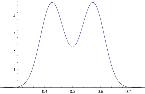
The other (small) term is expressed by:
| (8) | ||||
It contains the Erf-function neglected in and it is not far to the form even if now the term in the Erf-function differs by the positive constants . Near the strip borders, two of the constants are very similar and this term is positive (even if negligible).
The last term, indicated as Cauchy term, is:
| (9) | ||||
This term is different from zero also when all the . In this case the remaining term is the last line of the previous equation.
2.3 Examples and simulations
Figure 2 illustrates the various forms of and its splitting in two maximums around . For or the second maximum disappears.

Some simulations are constructed to test the results of the calculation. The parameters are from ref. [10]. Gaussian random noises are added to the to obtain the random values . The are inserted in equation 1 and the empirical PDF is compared with the analytical results. The simulations of figure 3 show a nice agreement.

The illustration of the soft switch-off of the second maximum is more difficult, because a detailed model of the modifications of the parameter are required. The trends of the of ref. [5] could be used in figure 4.

Symmetrically the maximum of rapidly disappears for impact points greater than , in the strip
2.4 The complete form of the COG3 PDF at the left border
The effects of the noise described for the right border of the strip are present even to the left border. Also here, the noise can promote the strip to become the seed strip. In this case the triplet of the algorithm become , the strips and the strip are the two lateral strips to the strip , This part of the COG3 PDF becomes:
| (10) |
As above, the second part of has its standard form in the reference centered on the strip , but the subtraction of one reports its form to that centered on the strip i.e. . With the usual constraints of ref. [1], this PDF becomes:
| (11) | ||||
The appropriate substitutions allow the use of equation 3 in these two new branches of the PDF. The first set of substitutions are: , and . These are essential to change the of equation 3 in the of equation 11. The second part of equation 11 is obtained from equation 3 with the substitutions: , , and . Equation 7 shows the practical use of these substitutions.
2.5 The use in the maximum likelihood search
The various sections of are relevant for the maximum likelihood search, even if they are invisible in the COG3 histograms. Typically, the experimental COG3 histograms have drops of data density near to or absence of data (gaps). The sectors of probabilities above or below have few or no data. Instead, our has a different aspect. This is due to the selection of the impact point as the event producing the noiseless signals modified by the noise. In the data, the strip of the hit is always supposed to be the seed of the cluster. Thus, the forms of the COG3 algorithm is always , where are the ordering of the strip signals around the seed strip . If near to the right-border of the strip, the noise promotes the nearby strip to becomes the seed strip, the COG3 becomes negative and greater than , instead of being greater than as calculated in . These apparent inconsistencies are irrelevant for the maximum likelihood search. The PDF, explored in the search, has always a fixed -value, given by the COG3 of the hit, and it is tested through the functions to find the most probable impact point. Hence, the search of the maximum of the PDF products must access the side of in the nearby strip with a continuous transition. The complex structure of the assures this continuity.
3 The error PDF of the four Strip COG (COG4)
The COG4 algorithm shares some similarities with the two-strip COG. It has a drop in the probability at for sufficiently wide signal distributions. Following our precedent convention, the ordering of the strips is with the reference system centered in the middle of the strip . The strip has a distance of 2 from the origin of the reference system, the strip has a distance -2. With these positions, the COG4 algorithm is defined as:
| (12) |
Before the study of the complete PDF for COG4, it is better to study an its partial form, limiting to the first part of ( in the following) neglecting the -function.
3.1 A partial expression for COG4 and its PDF for Gaussian noise
Similarly to the case of COG3, the simultaneous presence of the -function and the ratio of random variables does not allow to find a closed form of the PDF for Gaussian noise and approximations must be found. Instead, the partial form of COG4, without the -function, has an analytical expression, useful to select a good approximation for the complete PDF.
| (13) |
The substitution of variables, , , and with the Jacobian-determinant equal one, gives the integral of the Dirac- function in the form:
| (14) |
This equation is general and defined for any signal PDF. We calculate for a Gaussian additive noise supposed to perturb the signal collected by the strips with the form of equation 5. The Gaussian integrals have now analytic expressions. The absolute value of obliges to split the -integral in two parts that introduces a function . With the definition of , and as auxiliary variables:
The expressions of the results acquire a form with strong analogies with the COG3 PDFs. The main term has a Gaussian-like maximum centered on and the rest of the term contains a typical structure of differences. These differences are the noiseless COG4 calculated with the reference system centered on the strip , on the strip , on the strip and on the strip (a lucky suggestion of the MATHEMATICA function "FullSimplify"). The integration of equation 14 gives two terms, the first term is the main term :
| (15) | ||||
As previously, the second term is called Cauchy term, it survives when all the are zero:
| (16) | ||||
This form of the Cauchy term is different from the standard Cauchy PDF, but it has similar properties. Its cumulative distribution is an arctangent function as for a Cauchy PDF.
3.2 The complete PDF for the COG4 with the strip selection
The first part to be studied is the term:
| (18) |
The substitution of variables, , , , and with their Jacobian-determinant equal to one, allows a direct integration of the Dirac -function and to account for the .
| (19) |
With another substitution the equation 19 becomes:
| (20) |
The second part of this PDF (the left side) can be obtained in similar way with the corresponding variables or obtained with the substitutions , and . These equations are general for any probability , we calculate an explicit approximate expression for Gaussian PDFs.
3.3 Approximate expression for Gaussian noise
The integral on , as usual, creates many problems and impedes an analytical expression for the PDF. It conflicts with the that requires the splitting of the integral on . It was proved few times that the effect of the full account of is to assure the PDF to be a positive function. This condition can be released (with a small error) and reinserted at the end of the integration. To avoid an unmanageable number of terms in MATHEMATICA computation, it is better to start from the simpler PDF for the COG3 of ref. [1] observing that its integral coincides with that of equation 20 apart from a translation in ( for P1 and for P2). The addition of these translations to the main term of this closed form of COG3, and the neglect of its Erf-function, allows the computing of the remain two integrals without an explosion of the length of the MATHEMATICA outputs. As expected, the main term of the integrals of equation 20 is very similar to that of equation 15 the essential differences are the absence of the -function, giving to the factor of the exponential, and the presence of a
| (21) | ||||
where is defined as:
| (22) | ||||
The factor is essential to produce the drop of the PDF for with a smooth transition toward that dominates the for . Another term (Cauchy-like) is given by:
| (23) | ||||
We continue to indicate the term as a Cauchy term even if now it is a complicated function of . A different order of integration in equation 20 produces the main term with unimportant differences in the argument of the Erf-function and a different Cauchy term, always heavily suppressed by the exponential term. The left parts and are obtained from the previous equations with the indicated substitutions.

Figure 5 reports the comparison of the approximate expressions with a numerical integration of equation and a simulation constructed with identical data with the addition of a random Gaussian noise.
4 The error PDF for five-strip COG
The simplest form of the PDF for the five-strip COG (COG5) is defined. This COG5 could have the border gaps, as usual for the COG algorithms with an odd number of strips. In this case the gaps are relevant when the signal distribution is appreciably larger than four strips. We neglect such case. The general form of the COG5 is:
| (24) |
As always, the COG5 PDF is obtained with the integrals:
| (25) |
With the substitution of variables, , , , and and their Jacobian-determinant equal to one, the integration in of the Dirac -function gives:
| (26) |
This PDF can be used with any probability , we specialize it for Gaussian probabilities.
4.1 The for the Gaussian noise
The set of integrations in equation 26 have a closed form with an evident correlation with the expressions of the previously calculated PDFs. Due to the expressions we gave to the other exact PDFs, it is easy to anticipate the analytical expression of this PDF. A factor only ( in the following) has a non-easy relation to the precedent expressions. This factor is contained in the Erf function and in the Cauchy term. Even if the approximate expressions without the Erf functions work very well and the Cauchy term is negligible, for consistency this term must be calculated. The Gaussian integrals of equation 26 require further attentions to avoid the explosion of the number of terms in the exponents. MATHEMATICA is able to handle and to quickly simplify very long expressions as those of COG3. But, the lengths of the intermediate integrations become excessive for , to handle this case, many definitions of auxiliary variables must be introduced and few partial results must be simplified. The structure of equation 26 is very similar to equation 14 with the addition of another integration on . This set of integrals can be calculated in succession with the last integral on . The factor introduces the Erf-function that renders difficult further integrations.
To shorten the analytical expressions, the following auxiliary variables are very helpful:
and
the equation 26 for gives the most important term with the expression:
| (27) |
The approximate expression neglecting the Erf-term can be written easily. The approximation works very well. The Cauchy term is now:
| (28) |
This term has the functional dependence on in the denominator of equation 28 as a polynomial of second degree. Its cumulative function is always an arctangent as for the Cauchy PDF.
5 Conclusions
General expressions are reported for probability density functions of the center of gravity algorithms with three, four and five discretized values (strips for silicon detectors). These expressions are calculated with the method illustrated in a previous publication. Whenever possible, exact expressions for Gaussian noise are calculated. Approximate forms are constructed when the analytical integrations are impossible. The quality of these approximations are evaluated with comparisons with numerical integrations and data simulations. For the complete three strips and four strips probability distributions, exact analytical integrals are obtained neglecting the selection of the leading strips. These exact, but incomplete, expressions are useful to select good approximations. Even if our attention is directed to the center of gravity as a positioning algorithm in silicon micro-strip trackers, evidently these probability distributions have wider generality.
References
- [1] Landi G.; Landi G. E.; Probability Distributions of Positioning Errors for Some Forms of Center-of-Gravity Algorithms. arXiv:2004.08975 [physics.ins-det]
- [2] Landi G.; Landi G. E.; Positioning Error Probability for Some Forms of Center-of-Gravity Algorithms Calculated with the Cumulative Distributions. Part I. arXiv:2006.0000[physics.ins-det]
- [3] Archimedes; Geometrical solutions derived from mechanics Traslated from greek by J. L. Heiberg. Chicago 1909 in http://book.google.com
- [4] Galilei G.; Theoremata circa centrum gravitatis solidorum Firenze 1587
- [5] Landi G.; Landi G. E. Improvement of track reconstruction with well tuned probability distributions JINST 9 2014 P10006. arXiv:1404.1968[physics.ins-det] https://arxiv.org/abs/1404.1968
- [6] Landi, G.; Landi G. E. Optimizing momentum resolution with a new fitting method for silicon-strip detectors INSTRUMENTS 2018, 2(4), 22 https://doi.org/10.3390/instruments2040022
- [7] Landi G.; Landi G. E.; Beyond the -limit of the least squares resolution and the lucky-model arXiv:1808.06708[physics.ins-det] https://arxiv.org/abs/1808.06708.
- [8] Frühwirth R.; Regression with Gaussian mixture models applied to track fitting INSTRUMENTS 2020, 4(3) 25.
- [9] Landi G.; The center of gravity as an algorithm for position measurements Nucl. Instr. and Meth. A 485 (2002) 698 arXiv:1908.04447 [physics.ins-det] https://arxiv.org/abs/1910.04447.
- [10] Landi G.; Problems of position reconstruction in silicon microstrip detectors Nucl. Instr. and Meth. A 554 (2005) 226.
- [11] Landi G.; Landi G. E. The Cramer-Rao inequality to improve of the resolution of the least-squares method in track fitting INSTRUMENTS 2020, 4(1), 2; https://doi.org/10.3390/instruments4010002
- [12] Landi G.; Landi G. E. Generalized inequalities to optimize the fitting method for track reconstruction Physics 2020 2 608-623; https://doi.org/10.3390/physics2040035.
- [13] MATHEMATICA 6 Wolfram Inc. Champaign IL, USA
- [14] MatLab 8 The MathWork Inc. Natic, MA, USA