跳到论文正文
W Papers独立论文阅读器 arXiv:2011.14153 论文正文 计算阅读时间 · 0%
引用这篇论文根据当前论文元数据生成,正式投稿前建议核对。


License: arXiv.org perpetual non-exclusive license
arXiv:2011.14153v1 [math.PR] 28 Nov 2020

Brownian motion can feel the shape of a drum

Renan Gross Thanks: Weizmann Institute of Science. Email: renan.gross@weizmann.ac.il. Supported by the Adams Fellowship Program of the Israel Academy of Sciences and Humanities.
Abstract

We study the scenery reconstruction problem on the dd-dimensional torus, proving that a criterion on Fourier coefficients obtained by Matzinger and Lember (2006) for discrete cycles applies also in continuous spaces. In particular, with the right drift, Brownian motion can be used to reconstruct any scenery. To this end, we prove an injectivity property of an infinite Vandermonde matrix.

Keywords: Scenery reconstruction problem; infinite Vandermonde matrix; Brownian motion.

1 Introduction

1.1 Background

In its most general formulation, the scenery reconstruction problem asks the following: Let CC be a set, let be ff a function on CC, and (Xt)t≥0\left(X_{t}\right)_{t\geq 0} a stochastic process taking values in CC. What information can we learn about ff from the (infinite) trace f​(Xt)t≥0f\left(X_{t}\right)_{t\geq 0}? Can ff be completely reconstructed from this trace?

In one of the most common settings, CC is taken to be the discrete integer graph ℤ\mathbb{Z}, the function ff maps CC to {0,1}\left\{0,1\right\}, and XtX_{t} is a discrete-time random walk. For this model, numerous results exist in the literature for a variety of cases, e.g reconstruction when ff is random [1] and when ff is periodic. In the latter case, ff is essentially defined on a cycle of length ℓ\ell. Matzinger and Lember showed the following:

Theorem 1 ([5, Theorem 3.2]).

Let ff be a 22-coloring of the cycle of length ℓ\ell, and let XtX_{t} be a random walk with step distribution γ⁡(x)\gamma\left(x\right). If the Fourier coefficients {γ^​(k)}k=0ℓ−1\left\{\hat{\gamma}\left(k\right)\right\}_{k=0}^{\ell-1} are all distinct, then ff can be reconstructed from the trace f⁡(Xt)f\left(X_{t}\right).

Finucane, Tamuz and Yaari [3] considered the problem for finite Abelian groups, and showed that in many such cases, the above condition on the Fourier coefficients is necessary.

The problem can also be posed for a continuous space CC, such as ℝd\mathbb{R}^{d} or the torus 𝕋d\mathbb{T}^{d}, with XtX_{t} a continuous-time stochastic process. Here there has been considerably less work; to the best of our knowledge, at the time of writing this paper there are only two published results: Detecting “bells” [7] and reconstructing iterated Brownian motion [2]. See [4, 6] and references therein for an overview of the reconstruction problem, with a focus on ℤ\mathbb{Z} and ℤd\mathbb{Z}^{d}.

1.2 Results

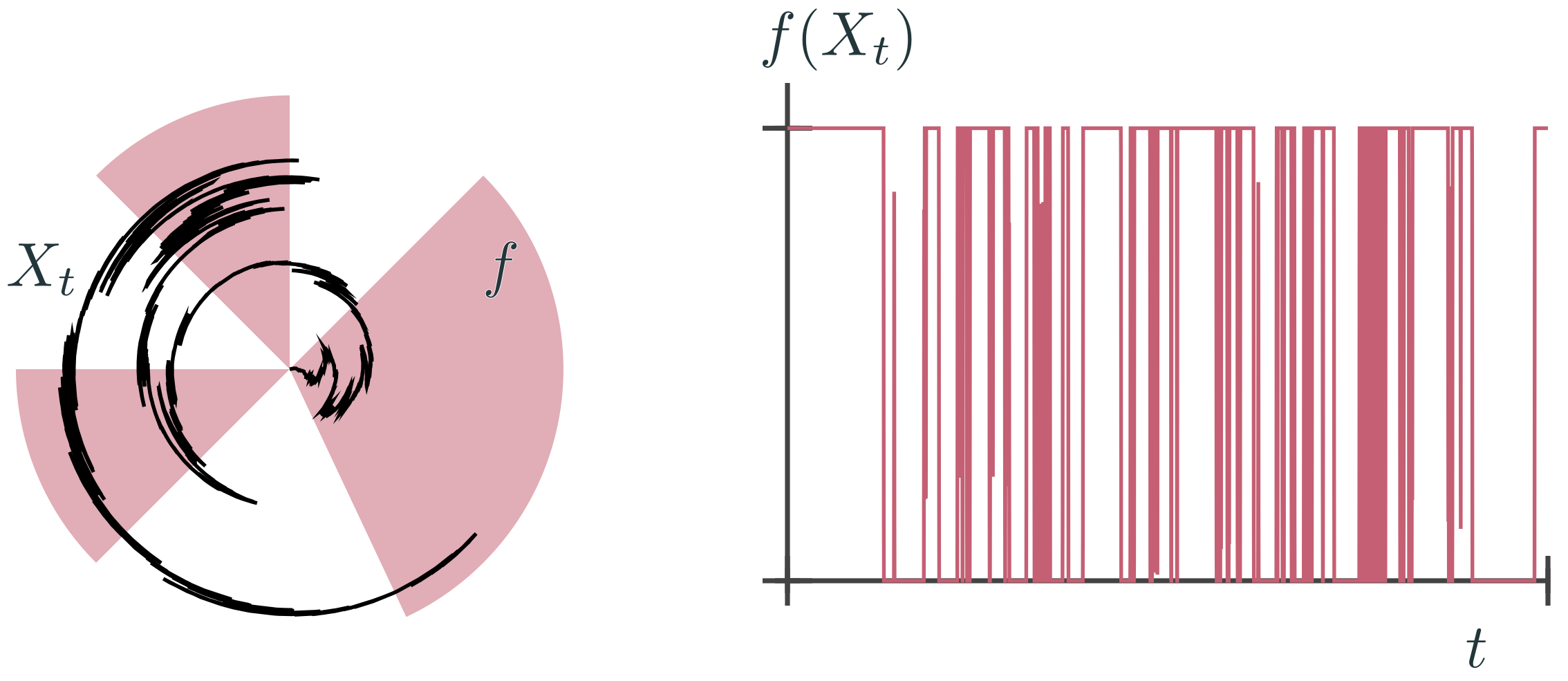
In this paper, we extend Theorem 1 from the discrete cycle to the continuous dd-dimensional torus 𝕋d=(ℝ/2​π​ℤ)d\mathbb{T}^{d}=\left(\mathbb{R}/2\pi\mathbb{Z}\right)^{d}. The discrete-time random walks are replaced by continuous-time processes XtX_{t} (such as Brownian motion), and the 22-colorings are replaced by the indicators ff of open sets. For an example of how the sample paths f⁡(Xt)f\left(X_{t}\right) might look like, see Figure 1, where ff is the indicator of a union of three intervals on the circle, and XtX_{t} is Brownian motion. The goal is to reconstruct the size and position of the intervals, up to rotations, from the trace f⁡(Xt)f\left(X_{t}\right).

Refer to caption
Figure 1: Left: Scenery reconstruction in one dimension. The black curve is a polar depiction of one-dimensional Brownian motion, with θ=Xt\theta=X_{t} and r=tr=\sqrt{t} (so that points near the center represent times close 00, and points near the edge represent larger times). The function ff is represented by the three shaded sectors. Right: The trace f⁡(Xt)f\left(X_{t}\right). It is equal to 11 precisely when the curve on the left is inside one of the shaded sectors.
Definition 2.

Let ℱ\mathcal{F} be a family of functions on the torus. The family ℱ\mathcal{F} is said to be reconstructible by XtX_{t} if there is a function A:ℝℝ+→ℝ𝕋dA:\mathbb{R}^{\mathbb{R}^{+}}\to\mathbb{R}^{\mathbb{T}^{d}} such that for every f∈ℱf\in\mathcal{F}, with probability 11 there exists a (random) shift θ∈𝕋d\theta\in\mathbb{T}^{d} such that A⁡(f⁡(Xt))​(x)=f⁡(x+θ)A\left(f\left(X_{t}\right)\right)\left(x\right)=f\left(x+\theta\right) for almost all xx.

For the particular case of d=1d=1, we also deal with reconstruction up to reflections:

Definition 3.

The family ℱ\mathcal{F} is said to be reconstructible up to reflections by XtX_{t}, if for all f∈ℱf\in\mathcal{F}, with probability 11 either A⁡(f⁡(Xt))​(x)=f⁡(x+θ)A\left(f\left(X_{t}\right)\right)\left(x\right)=f\left(x+\theta\right) for almost all xx, or A⁡(f⁡(Xt))​(x)=f⁡(−x+θ)A\left(f\left(X_{t}\right)\right)\left(x\right)=f\left(-x+\theta\right) for almost all xx.

In order to analyze the trace f⁡(Xt)f\left(X_{t}\right), we must of course have some control over the behavior of XtX_{t}. In this paper, we assume that XtX_{t} is an infinitely-divisible process with independent increments (this is the natural analog of a discrete-time random walk with independent steps). That is, there is a time-dependent distribution DtD_{t} on 𝕋d\mathbb{T}^{d} such that

  1. 1.

    Xt2−Xt1∼Dt2−t1X_{t_{2}}-X_{t_{1}}\sim D_{t_{2}-t_{1}} for every t2≥t1t_{2}\geq t_{1};

  2. 2.

    For all 0≤t1≤…≤tn0\leq t_{1}\leq\ldots\leq t_{n}, the increments Xt2−Xt1,…,Xtn−Xtn−1X_{t_{2}}-X_{t_{1}},\ldots,X_{t_{n}}-X_{t_{n-1}} are independent;

  3. 3.

    Dt+s=Dt⋆DsD_{t+s}=D_{t}\star D_{s} for every s,t≥0s,t\geq 0, where ⋆\star is the convolution operator.

We will also assume that DtD_{t} is either continuous, or that it is a mixture of an atom at 00 and a continuous distribution. In other words, writing DtD_{t} as a function of xx for simplicity, we have

Dt​(x)=βt​δ​(x)+(1−βt)​γt​(x),D_{t}\left(x\right)=\beta_{t}\delta\left(x\right)+\left(1-\beta_{t}\right)\gamma_{t}\left(x\right),

where δ⁡(x)\delta\left(x\right) is the Dirac δ\delta-distribution, γt\gamma_{t} is a probability density function, and βt∈[0,1]\beta_{t}\in\left[0,1\right] is a time dependent factor. We will also assume that γt\gamma_{t} is not too wild: γt∈L2​(𝕋d)\gamma_{t}\in\mathrm{L}^{2}\left(\mathbb{T}^{d}\right) for all t>0t>0.

Remark 4.

This class of distributions includes Brownian motion, and any Poisson process whose steps have an L2\mathrm{L}^{2} probability density function. It also contains the sum of Brownian motion and any arbitrary independent Poisson process, since the diffusion smooths out any irregularities in the jumps. It does not, however, contain general jump processes with atoms, even if the atoms are dense in 𝕋d\mathbb{T}^{d} (e.g a Poisson process on 𝕋\mathbb{T} which jumps by a step size α\alpha rationally independent from π\pi).

The functions we reconstruct will be the indicators of open sets, whose boundary has 00 measure in ℝd\mathbb{R}^{d}. Let

ℱd={𝟏x∈Ω​(x)∣Ω⊆𝕋d​ is open, ​Lebesgued​(∂Ω)=0}.\mathcal{F}_{d}=\left\{\mathbf{1}_{x\in\Omega}\left(x\right)\mid\Omega\subseteq\mathbb{T}^{d}\text{ is open, }\mathrm{Lebesgue}_{d}\left(\partial\Omega\right)=0\right\}.

Our main result is as follows:

Theorem 5 (General reconstruction).

Let XtX_{t} be a stochastic process on 𝕋d\mathbb{T}^{d} as above. If there exists a time t0t_{0} such that the Fourier coefficients {γ^t0​(k)}k∈ℤd\left\{\hat{\gamma}_{t_{0}}\left(k\right)\right\}_{k\in\mathbb{Z}^{d}} are all distinct and nonzero, then ℱd\mathcal{F}_{d} is reconstructible by XtX_{t}.

In one dimension, we show that symmetric distributions can reconstruct ℱ1\mathcal{F}_{1} up to reflections:

Theorem 6 (Symmetric reconstruction).

Let XtX_{t} be a stochastic process on 𝕋\mathbb{T} as above, and suppose that γt\gamma_{t} is symmetric, i.e γt​(y)=γt​(−y)\gamma_{t}\left(y\right)=\gamma_{t}\left(-y\right) for all yy. If there exists a time t0t_{0} such that the positive-indexed Fourier coefficients {γ^t0​(k)}k≥0\left\{\hat{\gamma}_{t_{0}}\left(k\right)\right\}_{k\geq 0} are all distinct and nonzero, then ℱ1\mathcal{F}_{1} is reconstructible up to reflections by XtX_{t}.

One corollary of Theorem 5, is that with the right drift, Brownian motion can be used to reconstruct ℱd\mathcal{F}_{d}.

Corollary 7 (Brownian motion can feel the shape of a drum).

Let XtX_{t} be Brownian motion with drift v∈ℝdv\in\mathbb{R}^{d}, such that {v1,…,vd}\left\{v_{1},\ldots,v_{d}\right\} are rationally independent. Then ℱd\mathcal{F}_{d} is reconstructible by XtX_{t}.

Remark 8.

The condition on the drift vv is natural: If the components of vv are rationally independent, then the geodesic flow defined by vv is dense in 𝕋d\mathbb{T}^{d}. Reconstructing a set Ω\Omega from this geodesic is immediate. In this sense, Corollary 7 states that reconstruction is possible also in the presence of noise which pushes us out of the trajectory. See Section 6 for a question on a related model.

The starting point for our results is a relation, introduced in [5], between two types of nn-point correlations related to ff - one known, and one unknown. After inverting the relation, the latter correlation can be used to reconstruct the function ff. In the discrete case, the relation is readily inverted using a finite Vandermonde matrix. In the continuous setting, additional difficulties arise due to both the more complicated nature of the distribution DtD_{t}, which mixes together different correlations, and the fact that the function space on 𝕋d\mathbb{T}^{d} is infinite-dimensional. To address the latter issue, we prove an injectivity result for infinite Vandermonde matrices, which may be of independent interest.

Lemma 9 (Infinite Vandermonde).

Let p,q∈[1,∞]p,q\in\left[1,\infty\right] be such that 1p+1q=1\frac{1}{p}+\frac{1}{q}=1. Let (zn)n∈ℓp​(ℂ)\left(z_{n}\right)_{n}\in\ell^{p}\left(\mathbb{C}\right) be a sequence of distinct complex numbers such that zn→0z_{n}\to 0, and zn≠0z_{n}\neq 0 for all nn. Let VV be the infinite Vandermonde matrix with znz_{n} as generators, i.e

Vi​j=zji.V_{ij}=z_{j}^{i}.

If 𝐱∈ℓq​(ℂ)\boldsymbol{x}\in\ell^{q}\left(\mathbb{C}\right) is a zero of the infinite system of equations

V​𝒙=0,V\boldsymbol{x}=0, (1)

then 𝐱=0\boldsymbol{x}=0.

Remark 10.

The matrix equation V​𝒙=0V\boldsymbol{x}=0 means that for every index i∈ℕi\in\mathbb{N} we have

0=∑j=1∞Vi​j​xj=∑j=1∞zji​xj.0=\sum_{j=1}^{\infty}V_{ij}x_{j}=\sum_{j=1}^{\infty}z_{j}^{i}x_{j}.

By Hölder’s inequality, since z∈ℓp​(ℂ)z\in\ell^{p}\left(\mathbb{C}\right) and 𝒙∈ℓq​(ℂ)\boldsymbol{x}\in\ell^{q}\left(\mathbb{C}\right), the series (zji​xj)j\left(z_{j}^{i}x_{j}\right)_{j} is absolutely convergent, and the left hand side of (1) is well defined.

Basic preliminaries and the proof of Theorem 5 are given in the next section. Section 3 gives the outline of Theorem 2, relying on the same techniques described in Section 2. Brownian motion is discussed in Section 4, and Lemma 9 is proved in Section 5. We conclude the paper with some open questions.

1.3 Acknowledgments

The author thanks Itai Benjamini, Ronen Eldan, Shay Sadovsky, Ori Sberlo and Ofer Zeitouni for their stimulating discussions and suggestions.

2 General reconstruction

2.1 Notation and simple properties of DtD_{t}

We write dd-dimensional vectors in standard italics, e.g k∈ℤdk\in\mathbb{Z}^{d}. Tuples of nn vectors are written in boldface, e.g 𝒌∈ℤn​d\boldsymbol{k}\in\mathbb{Z}^{nd}, with 𝒌=(k1,…,kn)\boldsymbol{k}=\left(k_{1},\ldots,k_{n}\right) and ki∈ℤdk_{i}\in\mathbb{Z}^{d}.

The Fourier series of a function g:𝕋d→ℂg:\mathbb{T}^{d}\to\mathbb{C} is a function g^:ℤd→ℂ\hat{g}:\mathbb{Z}^{d}\to\mathbb{C}, given by

g^(k)=∫𝕋dg(x)e−ik⋅xdx.\hat{g}\left(k\right)=\int_{\mathbb{T}^{d}}g\left(x\right)e^{-ik\cdot x}dx.

Note that we do not divide by the customary 1/(2​π)d1/\left(2\pi\right)^{d}. This simplifies the statement of the convolution theorem: In this setting, we have

f⋆g^=f^⋅g^,\widehat{f\star g}=\hat{f}\cdot\hat{g},

without any leading factor in the right hand side.

This definition also extends to the Dirac δ\delta-distribution, even though it is not a function, so that for all k∈ℤdk\in\mathbb{Z}^{d},

δ^(k)=∫−ππδ(x)e−ik⋅xdx=1.\hat{\delta}\left(k\right)=\int_{-\pi}^{\pi}\delta\left(x\right)e^{-ik\cdot x}dx=1.

Recall that Dt=βt​δ+(1−βt)​γtD_{t}=\beta_{t}\delta+\left(1-\beta_{t}\right)\gamma_{t}. Using the fact that Ds+t=Ds⋆DtD_{s+t}=D_{s}\star D_{t}, a short calculation shows that if the parameter βt\beta_{t} is not identically 00, it must decay exponentially: βt=e−c​t\beta_{t}=e^{-ct} for some constant cc. We implicitly assume that βt\beta_{t} is not identically 11, as in this case XtX_{t} does not move and is uninteresting. We thus have that

βα​t=βtα∀α,t>0.\beta_{\alpha t}=\beta_{t}^{\alpha}\,\,\,\,\,\,\,\forall\alpha,t>0. (2)

Since DtD_{t} has a probability density function γt\gamma_{t}, we have that Dt→U⁡(𝕋d)D_{t}\to U\left(\mathbb{T}^{d}\right) in distribution as t→∞t\to\infty, i.e XtX_{t} converges to the uniform distribution no matter its starting point.

The distribution DtD_{t} has a Fourier representation D^t\hat{D}_{t}, given by

D^t​(k)=βt​δ^​(k)+(1−βt)​γ^t​(k)=βt+(1−βt)​γ^t​(k)​k∈ℤd.\hat{D}_{t}\left(k\right)=\beta_{t}\hat{\delta}\left(k\right)+\left(1-\beta_{t}\right)\hat{\gamma}_{t}\left(k\right)=\beta_{t}+\left(1-\beta_{t}\right)\hat{\gamma}_{t}\left(k\right)\,\,\,\,\,k\in\mathbb{Z}^{d}. (3)

By the convolution theorem, D^t+s=Dt⋆Ds^=D^t​D^s\hat{D}_{t+s}=\widehat{D_{t}\star D_{s}}=\hat{D}_{t}\hat{D}_{s}. From this it follows that for any α,t>0\alpha,t>0, we have

D^α​t=(D^t)α.\hat{D}_{\alpha t}=\left(\hat{D}_{t}\right)^{\alpha}.

Plugging this into (3) gives

βα​t+(1−βα​t)​γ^α​t​(k)=(βt+(1−βt)​γ^t​(k))α,\beta_{\alpha t}+\left(1-\beta_{\alpha t}\right)\hat{\gamma}_{\alpha t}\left(k\right)=\left(\beta_{t}+\left(1-\beta_{t}\right)\hat{\gamma}_{t}\left(k\right)\right)^{\alpha},

and so by (2),

γ^α​t=(βt+(1−βt)​γ^t)α−βtα1−βtα.\hat{\gamma}_{\alpha t}=\frac{\left(\beta_{t}+\left(1-\beta_{t}\right)\hat{\gamma}_{t}\right)^{\alpha}-\beta_{t}^{\alpha}}{1-\beta_{t}^{\alpha}}. (4)

2.2 Proof of Theorem 5

The proofs of Theorems 5 and 6 use the relation between the spatial correlation and temporal correlation introduced in [5]. Let ff be the indicator of an open set Ω\Omega. For every integer n≥0n\geq 0, define the nn-th spatial correlation of ff, denoted Sn:𝕋n​d→ℝS_{n}:\mathbb{T}^{nd}\to\mathbb{R}, as

Sn​(𝒚)\displaystyle S_{n}\left(\boldsymbol{y}\right) =1(2​π)d∫𝕋df(x)f(x+y1)⋯f(x+∑i=1nyi)dx\displaystyle=\frac{1}{\left(2\pi\right)^{d}}\int_{\mathbb{T}^{d}}f\left(x\right)f\left(x+y_{1}\right)\cdots f\left(x+\sum_{i=1}^{n}y_{i}\right)dx
=1(2​π)d​∫𝕋df⁡(x)​∏k=1n[f⁡(x+∑i=1kyi)]​𝑑x,\displaystyle=\frac{1}{\left(2\pi\right)^{d}}\int_{\mathbb{T}^{d}}f\left(x\right)\prod_{k=1}^{n}\left[f\left(x+\sum_{i=1}^{k}y_{i}\right)\right]dx,

and the nn-th temporal correlation of f⁡(Xt)f\left(X_{t}\right), denoted Tn:ℝ+n→ℝT_{n}:\mathbb{R}_{+}^{n}\to\mathbb{R}, as

Tn(𝒕)=𝔼X0∼U⁡(𝕋d)[f(X0)f(Xt1)⋯f(X∑i=1nti)]T_{n}\left(\boldsymbol{t}\right)=\mathbb{E}_{X_{0}\sim U\left(\mathbb{T}^{d}\right)}\left[f\left(X_{0}\right)f\left(X_{t_{1}}\right)\cdots f\left(X_{\sum_{i=1}^{n}t_{i}}\right)\right]

(note that S0S_{0} and T0T_{0} are just constants, equal to the measure of Ω\Omega relative to 𝕋d\mathbb{T}^{d}). The proof involves two parts: The first shows that Sn​(𝒚)S_{n}\left(\boldsymbol{y}\right) can be calculated from our knowledge of Tn​(𝒕)T_{n}\left(\boldsymbol{t}\right). The second uses Sn​(𝒚)S_{n}\left(\boldsymbol{y}\right) to reconstruct ff with better and better precision as n→∞n\to\infty.

Proposition 11.

Let n∈ℕn\in\mathbb{N}. Under the conditions of Theorem 5, the function SnS_{n} can be calculated from f⁡(Xt)f\left(X_{t}\right) with probability 11.

We intend to prove Proposition 11 using the Vandermonde lemma (Lemma 9). To this end, we first show the following:

Proposition 12.

For every positive integers n,m∈ℕn,m\in\mathbb{N}, and every set of times t1,…,tn>0t_{1},\ldots,t_{n}>0, the value of the sum

∑𝒌∈ℤn​d(∏i=1nγ^ti​(ki))m​S^​(𝒌)\sum_{\boldsymbol{k}\in\mathbb{Z}^{nd}}\left(\prod_{i=1}^{n}\hat{\gamma}_{t_{i}}\left(k_{i}\right)\right)^{m}\hat{S}\left(\boldsymbol{k}\right)

can be calculated from f⁡(Xt)f\left(X_{t}\right) with probability 11.

Proof.

By (4), for every m∈ℕm\in\mathbb{N} and t>0t>0 we have

γ^m​t=(βt+(1−βt)​γ^t)m−βtm1−βtm.\hat{\gamma}_{mt}=\frac{\left(\beta_{t}+\left(1-\beta_{t}\right)\hat{\gamma}_{t}\right)^{m}-\beta_{t}^{m}}{1-\beta_{t}^{m}}.

Rearranging, we can write γ^tm\hat{\gamma}_{t}^{m} as a sum of smaller powers of γ^t\hat{\gamma}_{t}:

γ^tm=∑j=1m−1cj​γ^tj+γ^m​t,\hat{\gamma}_{t}^{m}=\sum_{j=1}^{m-1}c_{j}\hat{\gamma}_{t}^{j}+\hat{\gamma}_{mt},

where cjc_{j} are some coefficients (in particular, when DtD_{t} has no atom, i.e when βt=0\beta_{t}=0 for all t>0t>0, this sum is rather simple: γ^tm=γ^m​t\hat{\gamma}_{t}^{m}=\hat{\gamma}_{mt}). Reiterating this process, we find that the mm-th power of γ^t\hat{\gamma}_{t} can be written as some linear combination

γ^tm=∑j=1m−1cj′​γ^j​t.\hat{\gamma}_{t}^{m}=\sum_{j=1}^{m-1}c_{j}^{\prime}\hat{\gamma}_{jt}.

Thus, the product (∏i=1nγ^ti​(ki))m\left(\prod_{i=1}^{n}\hat{\gamma}_{t_{i}}\left(k_{i}\right)\right)^{m} is itself a sum of multilinear monomials in {γ^j​ti}j=1m−1\left\{\hat{\gamma}_{jt_{i}}\right\}_{j=1}^{m-1}, and so to prove the proposition it suffices to prove it for m=1m=1.

The temporal correlation Tn​(𝒕)T_{n}\left(\boldsymbol{t}\right) can be computed by the process f⁡(Xt)f\left(X_{t}\right): Since XtX_{t} approaches the uniform distribution on 𝕋d\mathbb{T}^{d} as t→0t\to 0, for any fixed times t1,…,tnt_{1},\ldots,t_{n}, we can choose sampling times τ1,τ2,…\tau_{1},\tau_{2},\ldots so that {f⁡(Xτj)​f​(Xτj+t1)​…​f​(Xτj+∑i=1nti)}j=1∞\left\{f\left(X_{\tau_{j}}\right)f\left(X_{\tau_{j}+t_{1}}\right)\ldots f\left(X_{\tau_{j}+\sum_{i=1}^{n}t_{i}}\right)\right\}_{j=1}^{\infty} have pairwise correlations that are arbitrarily small, and are arbitrarily close in distribution to f(X0)f(Xt1)⋯f(X∑i=1nti)f\left(X_{0}\right)f\left(X_{t_{1}}\right)\cdots f\left(X_{\sum_{i=1}^{n}t_{i}}\right) with X0∼U⁡(𝕋d)X_{0}\sim U\left(\mathbb{T}^{d}\right). The temporal correlation Tn​(𝒕)T_{n}\left(\boldsymbol{t}\right) is then given, with probability 11, by the sample average at times τj\tau_{j}.

A relation between the spatial and temporal correlation can be obtained as follows. First, since X0X_{0} is uniform on 𝕋d\mathbb{T}^{d} in the definition of Tn​(𝒕)T_{n}\left(\boldsymbol{t}\right),

Tn​(𝒕)=1(2​π)d​∫𝕋df⁡(x)​𝔼​[∏k=1nf⁡(X∑i=1kti)|X0=x]​𝑑x.T_{n}\left(\boldsymbol{t}\right)=\frac{1}{\left(2\pi\right)^{d}}\int_{\mathbb{T}^{d}}f\left(x\right)\mathbb{E}\left[\prod_{k=1}^{n}f\left(X_{\sum_{i=1}^{k}t_{i}}\right)\big|X_{0}=x\right]dx.

By conditioning on the event that between times ti−1t_{i-1} and tit_{i} the process took a step of size yiy_{i}, this is equal to

Tn​(𝒕)\displaystyle T_{n}\left(\boldsymbol{t}\right) =∫𝕋d∫𝕋n​d(∏i=1nDti​(yi))​(f⁡(x)​∏k=1n[f⁡(x+∑i=1kyi)])​𝑑𝒚​𝑑x\displaystyle=\int_{\mathbb{T}^{d}}\int_{\mathbb{T}^{nd}}\left(\prod_{i=1}^{n}D_{t_{i}}\left(y_{i}\right)\right)\left(f\left(x\right)\prod_{k=1}^{n}\left[f\left(x+\sum_{i=1}^{k}y_{i}\right)\right]\right)\boldsymbol{d}\boldsymbol{y}dx
=∫𝕋n​d(∏i=1nDti​(yi))​Sn​(𝒚)​𝑑𝒚.\displaystyle=\int_{\mathbb{T}^{nd}}\left(\prod_{i=1}^{n}D_{t_{i}}\left(y_{i}\right)\right)S_{n}\left(\boldsymbol{y}\right)\boldsymbol{dy}. (5)

Since Dt​(y)=βt​δ​(y)+(1−βt)​γt​(y)D_{t}\left(y\right)=\beta_{t}\delta\left(y\right)+\left(1-\beta_{t}\right)\gamma_{t}\left(y\right), the product inside the integral breaks into a sum, where, for each time step tit_{i}, we have to choose whether the process stayed in place (corresponding the δ⁡(yi)\delta\left(y_{i}\right)), or moved according to the density γti\gamma_{t_{i}}. Whenever we choose to stay in place, we shrink the number of spatial variables in our correlation, since Sn​(y1,…,yk,0,yk+2,…,yn)=Sn−1​(y1,…,yk,yk+2,…,yn)S_{n}\left(y_{1},\ldots,y_{k},0,y_{k+2},\ldots,y_{n}\right)=S_{n-1}\left(y_{1},\ldots,y_{k},y_{k+2},\ldots,y_{n}\right). We can thus go over all choices A⊆[n]A\subseteq\left[n\right] of indices of times when the process moved according to γt\gamma_{t}, giving

Tn​(𝒕)=∑A⊆[n]∏i∉Aβti​∏i∈A(1−βti)​∫𝕋|A|​d(∏i∈Aγti​(yi))​S|A|​(𝒚​ restricted to A)​(∏i∈Ad​yi).T_{n}\left(\boldsymbol{t}\right)=\sum_{A\subseteq\left[n\right]}\prod_{i\notin A}\beta_{t_{i}}\prod_{i\in A}\left(1-\beta_{t_{i}}\right)\int_{\mathbb{T}^{\left|A\right|d}}\left(\prod_{i\in A}\gamma_{t_{i}}\left(y_{i}\right)\right)S_{\left|A\right|}\left(\boldsymbol{y}\text{ restricted to $A$}\right)\left(\prod_{i\in A}dy_{i}\right).

The integral in this expression can be seen as an inner product between ∏i∈Aγti​(yi)\prod_{i\in A}\gamma_{t_{i}}\left(y_{i}\right) and S|A|​(𝒚)¯\overline{S_{\left|A\right|}\left(\boldsymbol{y}\right)} over the torus 𝕋|A|​d\mathbb{T}^{\left|A\right|d}. Since both γt\gamma_{t} and S|A|S_{\left|A\right|} are in L2\mathrm{L}^{2}(𝕋d)\left(\mathbb{T}^{d}\right), by Parseval’s theorem, we can therefore replace it by a sum over all Fourier coefficients 𝒌∈ℤ|A|​d\boldsymbol{k}\in\mathbb{Z}^{\left|A\right|d}:

Tn​(𝒕)=1(2​π)d​∑A⊆[n]∏i∉Aβti​∏i∈A(1−βti)​∑𝒌∈ℤ|A|​d(∏i∈Aγ^ti​(ki))​S^|A|​(𝒌​ restricted to A).T_{n}\left(\boldsymbol{t}\right)=\frac{1}{\left(2\pi\right)^{d}}\sum_{A\subseteq\left[n\right]}\prod_{i\notin A}\beta_{t_{i}}\prod_{i\in A}\left(1-\beta_{t_{i}}\right)\sum_{\boldsymbol{k}\in\mathbb{Z}^{\left|A\right|d}}\left(\prod_{i\in A}\hat{\gamma}_{t_{i}}\left(k_{i}\right)\right)\hat{S}_{\left|A\right|}\left(\boldsymbol{k}\text{ restricted to $A$}\right). (6)

With the above display, Proposition 12 follows quickly by induction on nn. For the case n=1n=1, we have

(2​π)d​T1​(t)=βt​S0+∑k∈ℤdγ^t​(k)​S^1​(k).\left(2\pi\right)^{d}T_{1}\left(t\right)=\beta_{t}S_{0}+\sum_{k\in\mathbb{Z}^{d}}\hat{\gamma}_{t}\left(k\right)\hat{S}_{1}\left(k\right).

Since S0=T0S_{0}=T_{0}, the value of ∑k∈ℤdγ^t​(k)​S^1​(k)\sum_{k\in\mathbb{Z}^{d}}\hat{\gamma}_{t}\left(k\right)\hat{S}_{1}\left(k\right) is known. The induction step for general nn is now immediate, since by (6) it is evident that Tn​(𝒕)T_{n}\left(\boldsymbol{t}\right) is a multilinear polynomial in γ^ti\hat{\gamma}_{t_{i}}, and all terms with degree strictly smaller than nn are known by the induction hypothesis. ∎

Proof of Proposition 11.

We will now show that for every n∈ℕn\in\mathbb{N}, the values

{∑𝒌∈ℤn​d(∏i=1nγ^ti(ki))mS^n(𝒌)∣m∈ℕ,t1,…,tn>0}\left\{\sum_{\boldsymbol{k}\in\mathbb{Z}^{nd}}\left(\prod_{i=1}^{n}\hat{\gamma}_{t_{i}}\left(k_{i}\right)\right)^{m}\hat{S}_{n}\left(\boldsymbol{k}\right)\mid m\in\mathbb{N},t_{1},\ldots,t_{n}>0\right\}

uniquely determine S^n​(𝒌)\hat{S}_{n}\left(\boldsymbol{k}\right). Proposition 11 then follows, since (as a quick, omitted, calculation shows) Sn​(𝒚)S_{n}\left(\boldsymbol{y}\right) is continuous on 𝕋d\mathbb{T}^{d}, and is thus completely determined by its Fourier coefficients.

Suppose that there exists a bounded function Qn​(𝒚)Q_{n}\left(\boldsymbol{y}\right) on 𝕋n​d\mathbb{T}^{nd} such that for all m∈ℕm\in\mathbb{N} and all times t1,…,tn>0t_{1},\ldots,t_{n}>0,

∑𝒌∈ℤn​d(∏i=1nγ^ti​(ki))m​S^n​(𝒌)=∑𝒌∈ℤn​d(∏i=1nγ^ti​(ki))m​Q^n​(𝒌).\sum_{\boldsymbol{k}\in\mathbb{Z}^{nd}}\left(\prod_{i=1}^{n}\hat{\gamma}_{t_{i}}\left(k_{i}\right)\right)^{m}\hat{S}_{n}\left(\boldsymbol{k}\right)=\sum_{\boldsymbol{k}\in\mathbb{Z}^{nd}}\left(\prod_{i=1}^{n}\hat{\gamma}_{t_{i}}\left(k_{i}\right)\right)^{m}\hat{Q}_{n}\left(\boldsymbol{k}\right).

Then, denoting x𝒌=S^n​(𝒌)−Q^n​(𝒌)x_{\boldsymbol{k}}=\hat{S}_{n}\left(\boldsymbol{k}\right)-\hat{Q}_{n}\left(\boldsymbol{k}\right), we have that

∑𝒌∈ℤn​d(∏i=1nγ^ti​(ki))m​x𝒌=0.\sum_{\boldsymbol{k}\in\mathbb{Z}^{nd}}\left(\prod_{i=1}^{n}\hat{\gamma}_{t_{i}}\left(k_{i}\right)\right)^{m}x_{\boldsymbol{k}}=0.

Note that x𝒌∈ℓ2​(ℂ)x_{\boldsymbol{k}}\in\ell^{2}\left(\mathbb{C}\right), since both SnS_{n} and QnQ_{n} are in L2​(𝕋d)\mathrm{L}^{2}\left(\mathbb{T}^{d}\right). We wish to use Lemma 9 to show that necessarily x𝒌=0x_{\boldsymbol{k}}=0.

To do this, we must choose the times tit_{i} so that the products ∏i=1nγ^ti​(ki)\prod_{i=1}^{n}\hat{\gamma}_{t_{i}}\left(k_{i}\right) are all non-zero and distinct. Then, setting z𝒌=∏i=1nγ^ti​(ki)z_{\boldsymbol{k}}=\prod_{i=1}^{n}\hat{\gamma}_{t_{i}}\left(k_{i}\right), we will have that z𝒌∈ℓ2​(ℂ)z_{\boldsymbol{k}}\in\ell^{2}\left(\mathbb{C}\right) (since γ^ti\hat{\gamma}_{t_{i}} are the Fourier coefficients of a square integrable function γti\gamma_{t_{i}}), z𝒌z_{\boldsymbol{k}} are all distinct, and z𝒌≠0z_{\boldsymbol{k}}\neq 0 for all k∈ℤn​dk\in\mathbb{Z}^{nd}, exactly meeting the requirements of the lemma with p=q=1/2p=q=1/2.

To choose the times tit_{i}, recall that by assumption, there exists a time t0t_{0} such that {γ^t0​(k)}k∈ℤd\left\{\hat{\gamma}_{t_{0}}\left(k\right)\right\}_{k\in\mathbb{Z}^{d}} are all distinct and nonzero. We will show that there exist numbers α1,…,αn>0\alpha_{1},\ldots,\alpha_{n}>0, so that if ti=αi​t0t_{i}=\alpha_{i}t_{0}, then the products {∏i=1nγ^ti​(ki)}𝒌∈ℤn​d\left\{\prod_{i=1}^{n}\hat{\gamma}_{t_{i}}\left(k_{i}\right)\right\}_{\boldsymbol{k}\in\mathbb{Z}^{nd}} satisfy the above requirements. By (4), for every αi\alpha_{i} we have

γ^αi​t0=(βt0+(1−βt0)​γ^t0)αi−βt0αi1−βt0αi.\hat{\gamma}_{\alpha_{i}t_{0}}=\frac{\left(\beta_{t_{0}}+\left(1-\beta_{t_{0}}\right)\hat{\gamma}_{t_{0}}\right)^{\alpha_{i}}-\beta_{t_{0}}^{\alpha_{i}}}{1-\beta_{t_{0}}^{\alpha_{i}}}. (7)

For a particular k∈ℤdk\in\mathbb{Z}^{d}, let Bk={α>0∣γ^α​t0​(k)=0}B_{k}=\left\{\alpha>0\mid\hat{\gamma}_{\alpha t_{0}}\left(k\right)=0\right\} be the set of “bad” multipliers for γ^t0​(k)\hat{\gamma}_{t_{0}}\left(k\right). The coefficient γ^α​t0​(k)\hat{\gamma}_{\alpha t_{0}}\left(k\right) can be 00 only if

(βt0+(1−βt0)​γ^t0​(k))αi−βt0αi=0,\left(\beta_{t_{0}}+\left(1-\beta_{t_{0}}\right)\hat{\gamma}_{t_{0}}\left(k\right)\right)^{\alpha_{i}}-\beta_{t_{0}}^{\alpha_{i}}=0,

and since γ^t0​(k)≠0\hat{\gamma}_{t_{0}}\left(k\right)\neq 0, the function

z↦(βt0+(1−βt0)​γ^t0​(k))z−βt0zz\mapsto\left(\beta_{t_{0}}+\left(1-\beta_{t_{0}}\right)\hat{\gamma}_{t_{0}}\left(k\right)\right)^{z}-\beta_{t_{0}}^{z}

is a non-constant holomorphic function of zz. The set of zeros BkB_{k} is thus isolated, and in particular countable.

Now let 𝒌≠𝒌′∈ℤn​d\boldsymbol{k}\neq\boldsymbol{k}^{\prime}\in\mathbb{Z}^{nd} be two different vectors, and let B𝒌,𝒌′=(∪i=1nBki)⋃(∪i=1nBki′)B_{\boldsymbol{k},\boldsymbol{k}^{\prime}}=\left(\cup_{i=1}^{n}B_{k_{i}}\right)\bigcup\left(\cup_{i=1}^{n}B_{k_{i}^{\prime}}\right) be the set of bad αi\alpha_{i}’s which cause one of the γ^αi​t0\hat{\gamma}_{\alpha_{i}t_{0}} to be 00. Let

R𝒌,𝒌′={𝜶∈ℝ>0n∣∀j​αj∉B𝒌,𝒌′​ and ​∏i=1nγ^αi​t0​(ki)=∏i=1nγ^αi​t0​(ki′)}.R_{\boldsymbol{k,k^{\prime}}}=\left\{\boldsymbol{\alpha}\in\mathbb{R}_{>0}^{n}\mid\forall j\,\alpha_{j}\notin B_{\boldsymbol{k},\boldsymbol{k}^{\prime}}\text{ and }\prod_{i=1}^{n}\hat{\gamma}_{\alpha_{i}t_{0}}\left(k_{i}\right)=\prod_{i=1}^{n}\hat{\gamma}_{\alpha_{i}t_{0}}\left(k_{i}^{\prime}\right)\right\}.

By (7), this means that for every 𝜶∈R𝒌,𝒌′\boldsymbol{\alpha}\in R_{\boldsymbol{k},\boldsymbol{k}^{\prime}},

∏i=1n(βt0+(1−βt0)​γ^t0​(ki))αi−βt0αi(1−βt0αi)−∏i=1n(βt0+(1−βt0)​γ^t0​(ki′))αi−βt0αi(1−βt0αi)=0.\prod_{i=1}^{n}\frac{\left(\beta_{t_{0}}+\left(1-\beta_{t_{0}}\right)\hat{\gamma}_{t_{0}}\left(k_{i}\right)\right)^{\alpha_{i}}-\beta_{t_{0}}^{\alpha_{i}}}{\left(1-\beta_{t_{0}}^{\alpha_{i}}\right)}-\prod_{i=1}^{n}\frac{\left(\beta_{t_{0}}+\left(1-\beta_{t_{0}}\right)\hat{\gamma}_{t_{0}}\left(k_{i}^{\prime}\right)\right)^{\alpha_{i}}-\beta_{t_{0}}^{\alpha_{i}}}{\left(1-\beta_{t_{0}}^{\alpha_{i}}\right)}=0.

Let i∗i^{*} be an index so that ki∗≠ki∗′k_{i^{*}}\neq k_{i^{*}}^{\prime}. Since none of the factors γ^αi​t0​(ki)\hat{\gamma}_{\alpha_{i}t_{0}}\left(k_{i}\right) or γ^αi​t0​(ki′)\hat{\gamma}_{\alpha_{i}t_{0}}\left(k_{i}^{\prime}\right) are 00 by choice of R𝒌,𝒌′R_{\boldsymbol{k},\boldsymbol{k}^{\prime}}, we can rearrange the above, yielding

1−(1+1−βt0βt0​γ^t0​(ki∗))αi∗1−(1+1−βt0βt0​γ^t0​(ki∗′))αi∗−∏i≠i∗(βt0+(1−βt0)​γ^t0​(ki′))αi−βt0αi(βt0+(1−βt0)​γ^t0​(ki))αi−βt0αi=0.\frac{1-\left(1+\frac{1-\beta_{t_{0}}}{\beta_{t_{0}}}\hat{\gamma}_{t_{0}}\left(k_{i^{*}}\right)\right)^{\alpha_{i^{*}}}}{1-\left(1+\frac{1-\beta_{t_{0}}}{\beta_{t_{0}}}\hat{\gamma}_{t_{0}}\left(k_{i^{*}}^{\prime}\right)\right)^{\alpha_{i^{*}}}}-\prod_{i\neq i^{*}}\frac{\left(\beta_{t_{0}}+\left(1-\beta_{t_{0}}\right)\hat{\gamma}_{t_{0}}\left(k_{i}^{\prime}\right)\right)^{\alpha_{i}}-\beta_{t_{0}}^{\alpha_{i}}}{\left(\beta_{t_{0}}+\left(1-\beta_{t_{0}}\right)\hat{\gamma}_{t_{0}}\left(k_{i}\right)\right)^{\alpha_{i}}-\beta_{t_{0}}^{\alpha_{i}}}=0.

For fixed {αi}i≠i∗\left\{\alpha_{i}\right\}_{i\neq i^{*}}, the expression on the left-hand side is a function of the form z↦1−az1−bz−cz\mapsto\frac{1-a^{z}}{1-b^{z}}-c. Since {γ^t0​(k)}k∈ℤd\left\{\hat{\gamma}_{t_{0}}\left(k\right)\right\}_{k\in\mathbb{Z}^{d}} are all distinct, a≠ba\neq b. Thus this map is a non-constant holomorphic function on ℂ\B𝒌,𝒌′\mathbb{C}\backslash B_{\boldsymbol{k},\boldsymbol{k}^{\prime}}, and so for any fixed choice of {αi}i≠i∗\left\{\alpha_{i}\right\}_{i\neq i^{*}}, has only countably many zeros, i.e only countably many choices for αi∗\alpha_{i^{*}}. The Lebesgue measure of R𝒌,𝒌′R_{\boldsymbol{k,k^{\prime}}} in ℝn\mathbb{R}^{n} is therefore 00. But the set of all α1,…,αn>0\alpha_{1},\ldots,\alpha_{n}>0 such that either there are two equal nonzero products in {∏i=1nγ^αi​t0​(ki)}𝒌∈ℤn​d\left\{\prod_{i=1}^{n}\hat{\gamma}_{\alpha_{i}t_{0}}\left(k_{i}\right)\right\}_{\boldsymbol{k}\in\mathbb{Z}^{nd}} or one of the products is itself 00 is the countable union

⋃𝒌,𝒌′∈ℤn​dR𝒌,𝒌′∪(⋃𝒌,𝒌′∈ℤn​d{(α1,…,αk)∣αi∈(Bki∪Bki′)}),\bigcup_{\boldsymbol{k},\boldsymbol{k^{\prime}}\in\mathbb{Z}^{nd}}R_{\boldsymbol{k},\boldsymbol{k^{\prime}}}\cup\left(\bigcup_{\boldsymbol{k},\boldsymbol{k}^{\prime}\in\mathbb{Z}^{nd}}\left\{\left(\alpha_{1},\ldots,\alpha_{k}\right)\mid\alpha_{i}\in\left(B_{k_{i}}\cup B_{k_{i}^{\prime}}\right)\right\}\right),

and so too has measure 00. In particular, there must exist α1,…,αn>0\alpha_{1},\ldots,\alpha_{n}>0 so that the products are distinct and nonzero, as needed. ∎

Proof of Theorem 5.

We now show that knowledge of Sn​(𝒚)S_{n}\left(\boldsymbol{y}\right) is enough to reconstruct ff up to a translation of the torus. The main idea is this. Suppose that Sn​(𝒚)>0S_{n}\left(\boldsymbol{y}\right)>0 for some given 𝒚∈ℝn​d\boldsymbol{y}\in\mathbb{R}^{nd}. Then ∫𝕋d∏k=0nf⁡(x+∑i=1kyi)​𝑑x>0\int_{\mathbb{T}^{d}}\prod_{k=0}^{n}f\left(x+\sum_{i=1}^{k}y_{i}\right)dx>0, which means that there exists a point x0∈𝕋dx_{0}\in\mathbb{T}^{d} such that f⁡(x0+∑i=1kyi)=1f\left(x_{0}+\sum_{i=1}^{k}y_{i}\right)=1 for all k=0,…,nk=0,\ldots,n. By considering only yiy_{i}’s which partition 𝕋d\mathbb{T}^{d} into a grid, we can get an approximation of Ω\Omega by taking the union of the grid blocks.

Let δm=2​π/m\delta_{m}=2\pi/m, let n=mdn=m^{d}, and consider the set 𝒴={𝒚∈δ⋅ℕn​d∣Sn​(𝒚)>0}\mathcal{Y}=\left\{\boldsymbol{y}\in\delta\cdot\mathbb{N}^{nd}\mid S_{n}\left(\boldsymbol{y}\right)>0\right\}. Note that (2​π)d​Sn​(𝟎)=∫𝕋df⁡(x)​𝑑x=μ⁡(Ω)\left(2\pi\right)^{d}S_{n}\left(\boldsymbol{0}\right)=\int_{\mathbb{T}^{d}}f\left(x\right)dx=\mu\left(\Omega\right) (where μ\mu is the Lebesgue measure), so if 𝒴={∅}\mathcal{Y}=\left\{\emptyset\right\} then Ω=∅\Omega=\emptyset, and ff is identically zero. We may therefore assume that 𝒴≠∅\mathcal{Y\neq\emptyset}.

Each vector 𝒚∈𝒴\boldsymbol{y}\in\mathcal{Y} defines a set of points G𝒚={∑i=1kyi∣k=0,…,n}G_{\boldsymbol{y}}=\left\{\sum_{i=1}^{k}y_{i}\mid k=0,\ldots,n\right\}, where the sum ∑i=1kyi\sum_{i=1}^{k}y_{i} is taken to be in the torus 𝕋d\mathbb{T}^{d}. Since δm\delta_{m} divides the side-length of the torus, G𝒚G_{\boldsymbol{y}} can be viewed as a subset of a dd-dimensional grid in 𝕋d\mathbb{T}^{d}, with the individual yiy_{i} serving as “pointer vectors” to the next point in the grid. The number of points in G𝒚G_{\boldsymbol{y}} depends on 𝒚\boldsymbol{y}: If 𝒚=0\boldsymbol{y}=0, for example, then G𝒚={0}G_{\boldsymbol{y}}=\left\{0\right\}; however, we can also choose 𝒚\boldsymbol{y} such that G𝒚=δ​ℤd∩𝕋dG_{\boldsymbol{y}}=\delta\mathbb{Z}^{d}\cap\mathbb{T}^{d}.

Let 𝒚∗∈𝒴\boldsymbol{y}^{*}\in\mathcal{Y} be such that |G𝒚∗|≥|G𝒚|\left|G_{\boldsymbol{y}*}\right|\geq\left|G_{\boldsymbol{y}}\right| for all 𝒚∈𝒴\boldsymbol{y}\in\mathcal{Y}, and let Gm∗=G𝒚∗G_{m}^{*}=G_{\boldsymbol{y}^{*}}, so that Gm∗G_{m}^{*} is a largest possible subset when the pointer vectors are taken from 𝒴\mathcal{Y}. Using Gm∗G_{m}^{*}, we can now define a rough, shifted approximation Ωm\Omega_{m} to the domain Ω\Omega: Letting Cd=[−12,12]dC_{d}=\left[-\frac{1}{2},\frac{1}{2}\right]^{d} be the unit dd-dimensional cube, we cover each point x∈Gm∗x\in G_{m}^{*} by the scaled cube δm​Cd\delta_{m}C_{d}:

Ωm=Gm∗+δm​Cd\Omega_{m}=G_{m}^{*}+\delta_{m}C_{d}

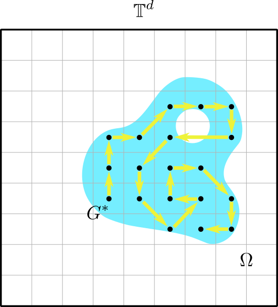
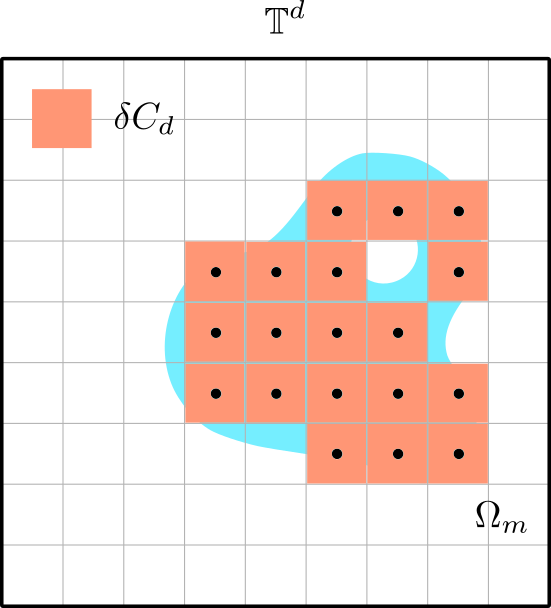
(here we use the Minkowski sum for the addition of two sets / the addition of a point and a set). See Figure 2 for an example of this procedure in 22 dimensions.

Refer to caption
Refer to caption
Figure 2: Left: The domain Ω\Omega (cyan), together with a maximal grid Gm∗G_{m}^{*} (black dots). The origin is shifted so that all grid points fall in Ω\Omega. The yellow vectors represent a possible choice for yiy_{i}. Right: The resultant approximation Ωm\Omega_{m}.

We now claim that Ωm→Ω\Omega_{m}\to\Omega up to translations, in the sense that there is a shift θ∈𝕋d\theta\in\mathbb{T}^{d} such that the symmetric difference vanishes: μ⁡((Ωm+θ)​Δ​Ω)→0\mu\left(\left(\Omega_{m}+\theta\right)\Delta\Omega\right)\to 0 as m→∞m\to\infty. To see this, let’s look separately at the contribution of (Ωm+θ)\Ω\left(\Omega_{m}+\theta\right)\backslash\Omega and the contribution of Ω\(Ωm+θ)\Omega\backslash\left(\Omega_{m}+\theta\right). First, as mentioned above, since Sn​(𝒚)>0S_{n}\left(\boldsymbol{y}\right)>0, there is a point xmx_{m} such that Gm∗+xm⊆ΩG_{m}^{*}+x_{m}\subseteq\Omega. Adding δm​Cd\delta_{m}C_{d} to both sides gives Ωm+xm⊆Ω+δm​Cd\Omega_{m}+x_{m}\subseteq\Omega+\delta_{m}C_{d}. We then have

μ⁡((Ωm+xm)\Ω)≤μ⁡((Ω+δm​Cd)\Ω)≤μ⁡(∂Ω+δm​Cd).\mu\left(\left(\Omega_{m}+x_{m}\right)\backslash\Omega\right)\leq\mu\left(\left(\Omega+\delta_{m}C_{d}\right)\backslash\Omega\right)\leq\mu\left(\partial\Omega+\delta_{m}C_{d}\right).

The latter expression goes to 00 as δm→0\delta_{m}\to 0, since

limm→∞μ⁡(∂Ω+δm​Cd)=μ⁡(⋂m(∂Ω+δm​Cd))=∂Ω is closedμ⁡(∂Ω)=0.\lim_{m\to\infty}\mu\left(\partial\Omega+\delta_{m}C_{d}\right)=\mu\left(\bigcap_{m}\left(\partial\Omega+\delta_{m}C_{d}\right)\right)\stackrel{{\scriptstyle\text{$\partial\Omega$ is closed}}}{{=}}\mu\left(\partial\Omega\right)=0.

Suppose now that x∈Ω\(Ωm+xm)x\in\Omega\backslash\left(\Omega_{m}+x_{m}\right), and let z∈δm​ℤd∩𝕋dz\in\delta_{m}\mathbb{Z}^{d}\cap\mathbb{T}^{d} be a grid-point closest to x−xmx-x_{m}. The point zz cannot be in Gm∗G_{m}^{*}: If it were, then the cube z+δm​Cdz+\delta_{m}C_{d} (which contains x−xmx-x_{m}) would be contained in Ωm\Omega_{m}, contradicting the fact that x∉Ωm+xmx\notin\Omega_{m}+x_{m}. Since |Gm∗|\left|G_{m}^{*}\right| is maximal, we necessarily have z+xm∉Ωz+x_{m}\notin\Omega (otherwise we could add it to Gm∗G_{m}^{*}). So every point not in Ωm+xm\Omega_{m}+x_{m} can be covered by placing the cube δm​Cd\delta_{m}C_{d} on some point in (Ω+xm)c\left(\Omega+x_{m}\right)^{c}. Thus

μ⁡(Ω\(Ωm+xm))\displaystyle\mu\left(\Omega\backslash\left(\Omega_{m}+x_{m}\right)\right) =μ⁡((Ωm+xm)c\Ωc)\displaystyle=\mu\left(\left(\Omega_{m}+x_{m}\right)^{c}\backslash\Omega^{c}\right)
≤μ⁡((Ωc+δm​Cd)\Ωc),\displaystyle\leq\mu\left(\left(\Omega^{c}+\delta_{m}C_{d}\right)\backslash\Omega^{c}\right),

and again the latter goes to 00 as δm→0\delta_{m}\to 0.

We thus have a sequence of vectors xm∈𝕋dx_{m}\in\mathbb{T}^{d} such that μ⁡((Ωm+xm)​Δ​Ω)→0\mu\left(\left(\Omega_{m}+x_{m}\right)\Delta\Omega\right)\to 0 as m→∞m\to\infty. Since 𝕋d\mathbb{T}^{d} is compact, xmx_{m} has a subsequence converging to some θ\theta, and it follows that μ⁡((Ωm+θ)​Δ​Ω)→0\mu\left(\left(\Omega_{m}+\theta\right)\Delta\Omega\right)\to 0 as well. ∎

3 Symmetric reconstruction

The proof of Theorem 6 is similar to that of Theorem 5. The main difference is that since γ^t​(k)=γ^t​(−k)\hat{\gamma}_{t}\left(k\right)=\hat{\gamma}_{t}\left(-k\right) for all kk, we cannot immediately use Lemma 9 to recover Sn​(𝒚)S_{n}\left(\boldsymbol{y}\right) anymore. This can be overcome by working with a completely symmetric version of Sn​(𝒚)S_{n}\left(\boldsymbol{y}\right), denoted σn​(𝒚)\sigma_{n}\left(\boldsymbol{y}\right) and defined as

σn​(𝒚)=∑𝜺∈{−1,1}nSn​(ε1​y1,…,εn​yn).\sigma_{n}\left(\boldsymbol{y}\right)=\sum_{\boldsymbol{\varepsilon}\in\left\{-1,1\right\}^{n}}S_{n}\left(\varepsilon_{1}y_{1},\ldots,\varepsilon_{n}y_{n}\right).
Proposition 13.

Under the conditions of Theorem 6, σn​(𝐲)\sigma_{n}\left(\boldsymbol{y}\right) can be calculated from f⁡(Xt)f\left(X_{t}\right) with probability 11.

Proof.

The proof uses the same techniques as that of Proposition 11; we highlight the differences here. Starting with the temporal-spatial relation (5),

Tn​(𝒕)\displaystyle T_{n}\left(\boldsymbol{t}\right) =∫𝕋n(∏i=1nDti​(yi))​Sn​(y1,…,yn)​𝑑𝒚,\displaystyle=\int_{\mathbb{T}^{n}}\left(\prod_{i=1}^{n}D_{t_{i}}\left(y_{i}\right)\right)S_{n}\left(y_{1},\ldots,y_{n}\right)\boldsymbol{dy},

observe that each integral of the form ∫−ππDti​(yi)​Sn​(y1,…,yn)​d​yi\int_{-\pi}^{\pi}D_{t_{i}}\left(y_{i}\right)S_{n}\left(y_{1},\ldots,y_{n}\right)dy_{i} can be split into two parts:

∫−ππDti​(yi)​Sn​(y1,…,yn)​d​yi=∫−π0Dti​(yi)​Sn​(y1,…,yn)​d​yi+∫0πDti​(yi)​Sn​(y1,…,yn)​d​yi,\int_{-\pi}^{\pi}D_{t_{i}}\left(y_{i}\right)S_{n}\left(y_{1},\ldots,y_{n}\right)dy_{i}=\int_{-\pi}^{0}D_{t_{i}}\left(y_{i}\right)S_{n}\left(y_{1},\ldots,y_{n}\right)dy_{i}+\int_{0}^{\pi}D_{t_{i}}\left(y_{i}\right)S_{n}\left(y_{1},\ldots,y_{n}\right)dy_{i},

where we use the convention that ∫−π0δ⁡(y)​g​(y)​𝑑y=12​limε→0+∫−πεδ⁡(y)​g​(y)​𝑑y=12​g​(0)\int_{-\pi}^{0}\delta\left(y\right)g\left(y\right)dy=\frac{1}{2}\lim_{\varepsilon\to 0^{+}}\int_{-\pi}^{\varepsilon}\delta\left(y\right)g\left(y\right)dy=\frac{1}{2}g\left(0\right). Making the change of variables yi→−yiy_{i}\to-y_{i} in the first integral and using the fact that DtD_{t} is symmetric, we thus have

∫−ππDti​(yi)​Sn​(y1,…,yn)​d​yi\displaystyle\int_{-\pi}^{\pi}D_{t_{i}}\left(y_{i}\right)S_{n}\left(y_{1},\ldots,y_{n}\right)dy_{i} =12​∫−ππDti​(yi)​[Sn​(y1,…,−yi,…,yn)+Sn​(y1,…,yi,…,yn)]​d​yi.\displaystyle=\frac{1}{2}\int_{-\pi}^{\pi}D_{t_{i}}\left(y_{i}\right)\left[S_{n}\left(y_{1},\ldots,-y_{i},\ldots,y_{n}\right)+S_{n}\left(y_{1},\ldots,y_{i},\ldots,y_{n}\right)\right]dy_{i}.

Performing this nn times yields

Tn​(𝒕)\displaystyle T_{n}\left(\boldsymbol{t}\right) =12n​∫𝕋n(∏i=1nDti​(yi))​σn​(𝒚)​𝑑𝒚.\displaystyle=\frac{1}{2^{n}}\int_{\mathbb{T}^{n}}\left(\prod_{i=1}^{n}D_{t_{i}}\left(y_{i}\right)\right)\sigma_{n}\left(\boldsymbol{y}\right)\boldsymbol{dy}. (8)

As in the proof of Proposition 12, this allows us to calculate the sum

∑𝒌∈ℤn(∏i=1nγ^ti​(ki))m​σ^n​(𝒌)\sum_{\boldsymbol{k}\in\mathbb{Z}^{n}}\left(\prod_{i=1}^{n}\hat{\gamma}_{t_{i}}\left(k_{i}\right)\right)^{m}\hat{\sigma}_{n}\left(\boldsymbol{k}\right)

for all n,m∈ℕn,m\in\mathbb{N} and every set of times t1,…,tn>0t_{1},\ldots,t_{n}>0. Now, both (∏i=1nγti​(yi))\left(\prod_{i=1}^{n}\gamma_{t_{i}}\left(y_{i}\right)\right) and σn​(𝒚)\sigma_{n}\left(\boldsymbol{y}\right) are symmetric in every coordinate yiy_{i}, and so the Fourier coefficients are invariant under flipping of individual entries. We can therefore restrict the sum to non-negative 𝒌\boldsymbol{k} vectors: Defining

αn​(𝒌)=2#​{i∣ki≠0}​σ^n​(𝒌),\alpha_{n}\left(\boldsymbol{k}\right)=2^{\#\left\{i\mid k_{i}\neq 0\right\}}\hat{\sigma}_{n}\left(\boldsymbol{k}\right),

we can calculate the sum

∑𝒌∈ℤ+n(∏i=1nγ^ti​(ki))m​αn​(𝒌)\sum_{\boldsymbol{k}\in\mathbb{Z}_{+}^{n}}\left(\prod_{i=1}^{n}\hat{\gamma}_{t_{i}}\left(k_{i}\right)\right)^{m}\alpha_{n}\left(\boldsymbol{k}\right)

for all n,m∈ℕn,m\in\mathbb{N} and times t1,…,tn>0t_{1},\ldots,t_{n}>0. As in the proof of Proposition 11, αn\alpha_{n} (and therefore σn\sigma_{n}) can be recovered from these quantities using Lemma 9, since by assumption there is a time t0t_{0} such that {γ^t0​(k)}k≥0\left\{\hat{\gamma}_{t_{0}}\left(k\right)\right\}_{k\geq 0} are all distinct and non-zero. ∎

Proposition 14.

Let δ>0\delta>0 divide 2​π2\pi. Given σn​(𝐲)\sigma_{n}\left(\boldsymbol{y}\right) for all n∈ℕn\in\mathbb{N} and 𝐲∈𝕋n\boldsymbol{y}\in\mathbb{T}^{n}, it is possible to calculate Sn​(𝐲)+Sn​(−𝐲)S_{n}\left(\boldsymbol{y}\right)+S_{n}\left(-\boldsymbol{y}\right) for all n∈ℕn\in\mathbb{N} and all 𝐲∈{(k1​δ,…,kn​δ)∣ki∈ℤ+}\boldsymbol{y}\in\left\{\left(k_{1}\delta,\ldots,k_{n}\delta\right)\mid k_{i}\in\mathbb{Z}_{+}\right\}.

Proof.

The proof is by induction. For n=1n=1, we just have σ1​(y)=S1​(y)+S1​(−y)\sigma_{1}\left(y\right)=S_{1}\left(y\right)+S_{1}\left(-y\right), and for general nn and 𝒌=𝟎\boldsymbol{k}=\boldsymbol{0}, we just have σn​(𝟎)=2n​Sn​(𝟎)\sigma_{n}\left(\boldsymbol{0}\right)=2^{n}S_{n}\left(\boldsymbol{0}\right). Now let n∈ℕn\in\mathbb{N} and 𝒌∈ℤ+n\boldsymbol{k}\in\mathbb{Z}_{+}^{n}. Assume that the statement holds true for nn for all vectors 𝒌′\boldsymbol{k}^{\prime} with ∑i=1nki′<∑i=1nki\sum_{i=1}^{n}k_{i}^{\prime}<\sum_{i=1}^{n}k_{i}, and also for all m<nm<n. We have

σn​(k1​δ,…,kn​δ)\displaystyle\sigma_{n}\left(k_{1}\delta,\ldots,k_{n}\delta\right) =∑𝜺∈{−1,1}nSn​(ε1​k1​δ,…,εn​kn​δ)\displaystyle=\sum_{\boldsymbol{\varepsilon}\in\left\{-1,1\right\}^{n}}S_{n}\left(\varepsilon_{1}k_{1}\delta,\ldots,\varepsilon_{n}k_{n}\delta\right)
=Sn​(k1​δ,…,kn​δ)+Sn​(−k1​δ,…,−kn​δ)+∑𝜺∈{−1,1}n,εi​ not all equalSn​(…).\displaystyle=S_{n}\left(k_{1}\delta,\ldots,k_{n}\delta\right)+S_{n}\left(-k_{1}\delta,\ldots,-k_{n}\delta\right)+\sum_{\boldsymbol{\varepsilon}\in\left\{-1,1\right\}^{n},\,\varepsilon_{i}\text{ not all equal}}S_{n}\left(\ldots\right).

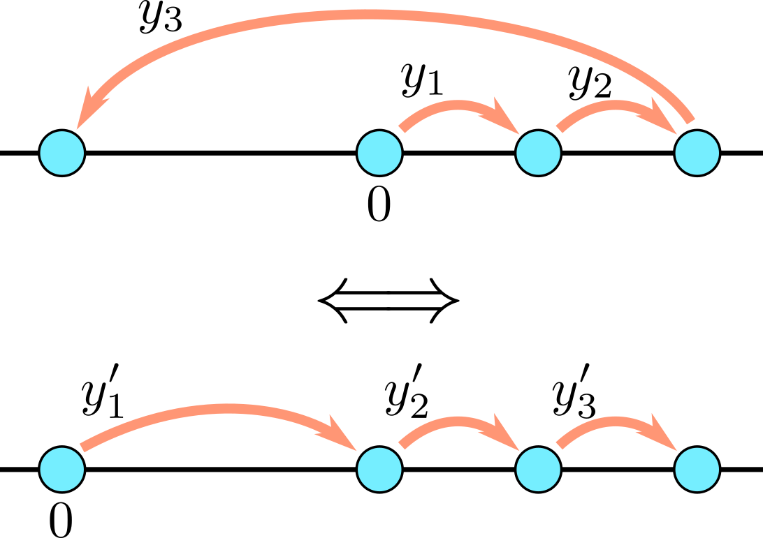
If not all εi\varepsilon_{i} are equal, then Sn​(ε1​k1​δ,…,εn​kn​δ)S_{n}\left(\varepsilon_{1}k_{1}\delta,\ldots,\varepsilon_{n}k_{n}\delta\right) is equal to some Sm​(k1′​δ,…,km′​δ)S_{m}\left(k^{\prime}_{1}\delta,\ldots,k_{m}^{\prime}\delta\right) for m≤nm\leq n: The total sum ∑iεi​ki\sum_{i}\varepsilon_{i}k_{i} is strictly smaller than ∑iki\sum_{i}k_{i}, and so the partial sums can be seen as the forward-only jumps of some 𝒚′\boldsymbol{y}^{\prime} with corresponding 𝒌′\boldsymbol{k}^{\prime} such that ∑iki′<∑iki\sum_{i}k_{i}^{\prime}<\sum_{i}k_{i} (the strict m<nm<n case is when the partial sums ∑εi​ki\sum\varepsilon_{i}k_{i} themselves are not unique). See Figure 3 for a visualization. Similarly, Sn​(−ε1​k1​δ,…,−εn​kn​δ)=−Sm​(−k1′​δ,…,−km′​δ)S_{n}\left(-\varepsilon_{1}k_{1}\delta,\ldots,-\varepsilon_{n}k_{n}\delta\right)=-S_{m}\left(-k^{\prime}_{1}\delta,\ldots,-k_{m}^{\prime}\delta\right). Since the sum over all εi\varepsilon_{i} can be split into polar pairs, by the induction hypothesis we can calculate the sum ∑𝜺∈{−1,1}n,εi​ not all equalSn\sum_{\boldsymbol{\varepsilon}\in\left\{-1,1\right\}^{n},\,\varepsilon_{i}\text{ not all equal}}S_{n}, and therefore also Sn​(k1​δ,…,kn​δ)+Sn​(−k1​δ,…,−kn​δ).S_{n}\left(k_{1}\delta,\ldots,k_{n}\delta\right)+S_{n}\left(-k_{1}\delta,\ldots,-k_{n}\delta\right).

Refer to caption
Figure 3: S3​(y1,y2,y3)=S3​(y1′,y2′,y3′)S_{3}\left(y_{1},y_{2},y_{3}\right)=S_{3}\left(y_{1}^{\prime},y_{2}^{\prime},y_{3}^{\prime}\right). The choice of origin does not matter, since SnS_{n} integrates over all 𝕋\mathbb{T} anyway. The total length y1′+y2′+y3′y_{1}^{\prime}+y_{2}^{\prime}+y_{3}^{\prime} is smaller than y1+y2+y3y_{1}+y_{2}+y_{3}.

∎

Proof sketch of Theorem 6.

Similarly to the proof of Theorem 5, once we know Sn​(k1​δ,…,kn​δ)+Sn​(−k1​δ,…,−kn​δ)S_{n}\left(k_{1}\delta,\ldots,k_{n}\delta\right)+S_{n}\left(-k_{1}\delta,\ldots,-k_{n}\delta\right), for every δn=2​π/n\delta_{n}=2\pi/n we can construct a set Ωn\Omega_{n} according a 𝒚∈{𝒚∈δ⋅ℕn∣Sn​(𝒚)+Sn​(−𝒚)>0}\boldsymbol{y}\in\left\{\boldsymbol{y}\in\delta\cdot\mathbb{N}^{n}\mid S_{n}\left(\boldsymbol{y}\right)+S_{n}\left(-\boldsymbol{y}\right)>0\right\} which maximizes G𝒚G_{\boldsymbol{y}}. The resulting fnf_{n} contains a subsequence which converges to either f⁡(x)f\left(x\right) or f⁡(−x)f\left(-x\right), where the ambiguity is because we do not know which of the two of Sn​(𝒚)S_{n}\left(\boldsymbol{y}\right) and Sn​(−𝒚)S_{n}\left(-\boldsymbol{y}\right) was greater than 00. ∎

4 Example: Brownian motion

4.1 Proof of Corollary 7

Proof.

For d=1d=1, the step distribution γt\gamma_{t} of Brownian motion on 𝕋\mathbb{T} is that of a wrapped normal distribution with drift, and is given by

γt(y)=12​t​π∑m=−∞∞e−(y−vt+2πm)2/2t.\gamma_{t}\left(y\right)=\frac{1}{\sqrt{2t\pi}}\sum_{m=-\infty}^{\infty}e^{-\left(y-vt+2\pi m\right)^{2}/2t}.

The Fourier coefficients of γt​(y)\gamma_{t}\left(y\right) can readily be calculated, by observing that the wrap-around gives the continuous Fourier transform evaluated at integer points:

γ^t​(k)\displaystyle\hat{\gamma}_{t}\left(k\right) =∫−ππe−i​k​y12​t​π∑m=−∞∞e−(y−vt+2πm)2/2tdy\displaystyle=\int_{-\pi}^{\pi}e^{-iky}\frac{1}{\sqrt{2t\pi}}\sum_{m=-\infty}^{\infty}e^{-\left(y-vt+2\pi m\right)^{2}/2t}dy
=∫−∞∞e−i​k​y12​t​πe−(y−vt)2/2tdy\displaystyle=\int_{-\infty}^{\infty}e^{-iky}\frac{1}{\sqrt{2t\pi}}e^{-\left(y-vt\right)^{2}/2t}dy
=e−i​v​t​k​e−2​t​π2​k2.\displaystyle=e^{-ivtk}e^{-2t\pi^{2}k^{2}}.

For standard Brownian motion, without drift, the coefficients are symmetric, but {γ^t​(k)}k≥0\left\{\hat{\gamma}_{t}\left(k\right)\right\}_{k\geq 0} are all distinct, and so by Theorem 6, reconstruction is possible using Brownian motion up to rotations and reflections.

The drift, however, can make the coefficients distinct. For d=1d=1, any non-zero drift will do, and reconstruction is possible up to rotations. In the general case, the Fourier coefficients of γt\gamma_{t} are

γ^t(k)=e−it∑j=1dvj⋅kje−2tπ2∑jkj2;k∈ℤd.\hat{\gamma}_{t}\left(k\right)=e^{-it\sum_{j=1}^{d}v_{j}\cdot k_{j}}e^{-2t\pi^{2}\sum_{j}k_{j}^{2}}\,\,\,\,;\,\,\,k\in\mathbb{Z}^{d}.

In order for the coefficients to be distinct, it suffices to make the factors e−it∑j=1dvj⋅kje^{-it\sum_{j=1}^{d}v_{j}\cdot k_{j}} all distinct, i.e there should exist a time tt such that for every k≠k′∈ℤdk\neq k^{\prime}\in\mathbb{Z}^{d} and every m∈ℤm\in\mathbb{Z},

∑j=1dvj​(kj−kj′)≠2​π​m/t.\sum_{j=1}^{d}v_{j}\left(k_{j}-k_{j}^{\prime}\right)\neq 2\pi m/t.

Choosing tt so that {v1,…,vd,2​πt}\left\{v_{1},\ldots,v_{d},\frac{2\pi}{t}\right\} are all rationally independent completes the proof. ∎

4.2 An explicit inversion

As a side note, we would like to mention that for Brownian motion, inverting the symmetric integral (8) (note the changed range of integration),

Tn​(𝒕)=∫[0,π]n(∏i=1nγti​(yi))​σn​(𝒚)​𝑑𝒚,T_{n}\left(\boldsymbol{t}\right)=\int_{\left[0,\pi\right]^{n}}\left(\prod_{i=1}^{n}\gamma_{t_{i}}\left(y_{i}\right)\right)\sigma_{n}\left(\boldsymbol{y}\right)\boldsymbol{dy},

is possible without resorting to Lemma 9: There exists an explicit relation between σn​(𝒚)\sigma_{n}\left(\boldsymbol{y}\right) and Tn​(𝒕)T_{n}\left(\boldsymbol{t}\right). The relation appears in (e.g) [8, 3.2-6, item 21]. We repeat the arguments here for completeness.

If we treat σn​(𝒚)\sigma_{n}\left(\boldsymbol{y}\right) as a periodic function over all ℝn\mathbb{R}^{n} where every coordinate has period 2​π2\pi, we can replace the folded normal distribution γt\gamma_{t} with a normal distribution over all ℝ+\mathbb{R}_{+}:

Tn​(𝒕)=∫𝒚∈ℝ+n(∏i=1n12​π​ti​e−yi22​ti)​σn​(𝒚)​𝑑𝒚.T_{n}\left(\boldsymbol{t}\right)=\int_{\boldsymbol{y}\in\mathbb{R}_{+}^{n}}\left(\prod_{i=1}^{n}\frac{1}{\sqrt{2\pi t_{i}}}e^{-\frac{y_{i}^{2}}{2t_{i}}}\right)\sigma_{n}\left(\boldsymbol{y}\right)\boldsymbol{dy}.

Let 𝒑∈ℝ+n\boldsymbol{p}\in\mathbb{R}_{+}^{n}. Multiplying both sides by e−p1​t1−…−pn−1​tn−1e^{-p_{1}t_{1}-\ldots-p_{n-1}t_{n-1}} and integrating all tit_{i}s from 00 to ∞\infty, we get

ℒ​{Tn}​(𝒑)=∫𝒕∈ℝ+n∫𝒚∈ℝ+n(∏i=1n12​π​ti​e−yi22​ti​e−pi​ti)​σn​(𝒚)​𝑑𝒚​𝑑𝒕,\mathcal{L}\left\{T_{n}\right\}\left(\boldsymbol{p}\right)=\int_{\boldsymbol{t}\in\mathbb{R}_{+}^{n}}\int_{\boldsymbol{y}\in\mathbb{R}_{+}^{n}}\left(\prod_{i=1}^{n}\frac{1}{\sqrt{2\pi t_{i}}}e^{-\frac{y_{i}^{2}}{2t_{i}}}e^{-p_{i}t_{i}}\right)\sigma_{n}\left(\boldsymbol{y}\right)\boldsymbol{dy}\boldsymbol{dt},

where ℒ​{f}\mathcal{L}\left\{f\right\} is the Laplace transform of ff. The individual integrals over tit_{i} in the right hand side can be readily calculated to be:

∫0∞e−p​t−y2/2​t​12​π​t​𝑑t=12​p​e−2​p​y.\int_{0}^{\infty}e^{-pt-y^{2}/2t}\frac{1}{\sqrt{2\pi t}}dt=\frac{1}{\sqrt{2p}}e^{-\sqrt{2p}y}.

This gives

ℒ​{Tn}​(𝒑)=∫ℝ+n(∏i=1n12​pi​e−2​pi​y)​σn​(𝒚)​𝑑𝒚.\mathcal{L}\left\{T_{n}\right\}\left(\boldsymbol{p}\right)=\int_{\mathbb{R}_{+}^{n}}\left(\prod_{i=1}^{n}\frac{1}{\sqrt{2p_{i}}}e^{-\sqrt{2p_{i}}y}\right)\sigma_{n}\left(\boldsymbol{y}\right)\boldsymbol{dy}.

Up to a change of variables si=2​pis_{i}=\sqrt{2p_{i}}, the right hand side is the Laplace transform of σn​(𝒚)\sigma_{n}\left(\boldsymbol{y}\right). Thus

σn=ℒ−1​{(∏i=1nsi)​ℒ​{Tn}​(12​s12,…,12​sn2)}.\sigma_{n}=\mathcal{L}^{-1}\left\{\left(\prod_{i=1}^{n}s_{i}\right)\mathcal{L}\left\{T_{n}\right\}\left(\frac{1}{2}s_{1}^{2},\ldots,\frac{1}{2}s_{n}^{2}\right)\right\}.

5 Proof of Lemma 9

Proof.

As noted in Remark 10, the equality V​𝒙=0V\boldsymbol{x}=0 means that for every index i∈ℕi\in\mathbb{N} we have

0=∑j=1∞Vi​j​xj=∑j=1∞zji​xj.0=\sum_{j=1}^{\infty}V_{ij}x_{j}=\sum_{j=1}^{\infty}z_{j}^{i}x_{j}. (9)

Since 𝒛∈ℓp​(ℂ)\boldsymbol{z}\in\ell^{p}\left(\mathbb{C}\right) and 𝒙∈ℓq​(ℂ)\boldsymbol{x}\in\ell^{q}\left(\mathbb{C}\right), by Hölder’s inequality the series (zji​xj)j\left(z_{j}^{i}x_{j}\right)_{j} is absolutely convergent for all ii, and we can change the order of summation; without loss of generality we can assume that znz_{n} are ordered so that |z1|≥|z2|≥…\left|z_{1}\right|\geq\left|z_{2}\right|\geq\ldots.

Assume by induction that x1,…,xkx_{1},\ldots,x_{k} have already been shown to be equal to 00, and let ℓ>0\ell>0 be such that |zk+1|,…,|zk+ℓ|\left|z_{k+1}\right|,\ldots,\left|z_{k+\ell}\right| are all of equal magnitudes, but |zk+ℓ|>|zk+ℓ+1|\left|z_{k+\ell}\right|>\left|z_{k+\ell+1}\right|. Since zn→0z_{n}\to 0, ℓ\ell is necessarily finite. For any fixed ii, the sum (9) can then be split into two parts:

∑s=1ℓzk+si​xk+s+∑j>k+ℓzji​xj=0.\sum_{s=1}^{\ell}z_{k+s}^{i}x_{k+s}+\sum_{j>k+\ell}z_{j}^{i}x_{j}=0.

Dividing by zk+ℓiz_{k+\ell}^{i} and denoting ωs=zk+szk+ℓ\omega_{s}=\frac{z_{k+s}}{z_{k+\ell}}, we have

∑s=1ℓωsi​xk+s+∑j>k+ℓ(zjzk+ℓ)i​xj=0.\sum_{s=1}^{\ell}\omega_{s}^{i}x_{k+s}+\sum_{j>k+\ell}\left(\frac{z_{j}}{z_{k+\ell}}\right)^{i}x_{j}=0.

Consider the ℓ\ell equations of the above form for i=r⋅mi=r\cdot m, where r=1,…,ℓr=1,\ldots,\ell and mm is a large number. In matrix form, this system of ℓ\ell equations can be written as

Vm​𝒙~+𝒖=0,V_{m}\tilde{\boldsymbol{x}}+\boldsymbol{u}=0, (10)

where:

  1. 1.

    VmV_{m} is a finite ℓ×ℓ\ell\times\ell Vandermonde matrix with generators ωsm=(zk+szk+ℓ)m\omega_{s}^{m}=\left(\frac{z_{k+s}}{z_{k+\ell}}\right)^{m}, s=1,…,ℓs=1,\ldots,\ell.

  2. 2.

    𝒙~\tilde{\boldsymbol{x}} is a vector of size ℓ\ell with x~s=xk+s\tilde{x}_{s}=x_{k+s} for s=1,…,ℓs=1,\ldots,\ell.

  3. 3.

    𝒖\boldsymbol{u} is a vector of length ℓ\ell with entries ur=∑j>k+ℓ(zjzk+ℓ)r​m​xju_{r}=\sum_{j>k+\ell}\left(\frac{z_{j}}{z_{k+\ell}}\right)^{rm}x_{j} for r=1,…,ℓr=1,\ldots,\ell. By our ordering and choice of ℓ\ell, |zk+ℓ|>|zj|\left|z_{k+\ell}\right|>\left|z_{j}\right| for j>k+ℓj>k+\ell, and we can factor out an exponentially decreasing term from each summand:

    |ur|\displaystyle\left|u_{r}\right| ≤|zk+ℓ+1zk+ℓ|r​m​∑j>k+ℓ|zjzk+ℓ+1|r​m​|xj|\displaystyle\leq\left|\frac{z_{k+\ell+1}}{z_{k+\ell}}\right|^{rm}\sum_{j>k+\ell}\left|\frac{z_{j}}{z_{k+\ell+1}}\right|^{rm}\left|x_{j}\right|
    (Hölder’s inequality)\displaystyle\left(\text{H\"{o}lder's inequality}\right) ≤|zk+ℓ+1zk+ℓ|r​m​(∑j>k+ℓ|zjzk+ℓ+1|p​r​m)1/p​‖𝒙‖q.\displaystyle\leq\left|\frac{z_{k+\ell+1}}{z_{k+\ell}}\right|^{rm}\left(\sum_{j>k+\ell}\left|\frac{z_{j}}{z_{k+\ell+1}}\right|^{prm}\right)^{1/p}\left\|\boldsymbol{x}\right\|_{q}.

    The sum ∑j>k+ℓ|zjzk+ℓ+1|p​r​m\sum_{j>k+\ell}\left|\frac{z_{j}}{z_{k+\ell+1}}\right|^{prm} is finite since 𝒛∈ℓp​(ℂ)\boldsymbol{z}\in\ell^{p}\left(\mathbb{C}\right), and is in fact uniformly bounded as a function of mm, since every summand has magnitude less than or equal to 11. Since |zk+ℓ+1|<|zk+ℓ|\left|z_{k+\ell+1}\right|<\left|z_{k+\ell}\right|, the term |zk+ℓ+1zk+ℓ|r​m\left|\frac{z_{k+\ell+1}}{z_{k+\ell}}\right|^{rm} goes to 00 as m→∞m\to\infty, and so the entries of 𝒖\boldsymbol{u} also decrease to 00 as m→∞m\to\infty.

The generators of VmV_{m} are all distinct, and so VmV_{m} is invertible. Equation (10) thus gives

𝒙~=−Vm−1​𝒖.\tilde{\boldsymbol{x}}=-V_{m}^{-1}\boldsymbol{u}.

As mentioned in item (3), the entries of 𝒖\boldsymbol{u} decay to 00 in mm. To show that 𝒙~=0\boldsymbol{\tilde{x}}=0 (and thus all of xk+s=0x_{k+s}=0 for s=1,…,ℓs=1,\ldots,\ell), it therefore suffices to uniformly bound the infinity-norm ‖Vm−1‖∞\left\|V_{m}^{-1}\right\|_{\infty} for infinitely many mm. Recall that the inverse of the ℓ×ℓ\ell\times\ell Vandermonde matrix with generators ωsm\omega_{s}^{m} has entries

(Vm−1)i​j=(−1)j−1​Ci​jωim​∏k≠i1≤k≤ℓ(ωim−ωkm),\left(V_{m}^{-1}\right)_{ij}=\left(-1\right)^{j-1}\dfrac{C_{ij}}{\omega_{i}^{m}\prod_{\stackrel{{\scriptstyle 1\leq k\leq\ell}}{{k\neq i}}}\left(\omega_{i}^{m}-\omega_{k}^{m}\right)}, (11)

where

Ci​j={∑m1,…,mℓ−j≠i1≤k1<…<kn−j≤ℓωm1⋯ωmℓ−j1≤j<ℓ1j=ℓ.C_{ij}=\begin{cases}\sum_{\stackrel{{\scriptstyle 1\leq k_{1}<\ldots<k_{n-j}\leq\ell}}{{m_{1},\ldots,m_{\ell-j}\neq i}}}\omega_{m_{1}}\cdots\omega_{m_{\ell-j}}&1\leq j<\ell\\ 1&j=\ell.\end{cases}

Since the generators ωsm\omega_{s}^{m} are all on the unit circle, the numerator Ci​jC_{ij} is always bounded by a constant independent of mm. For the denominator, it suffices to show that we can choose infinitely many mm such that |ωim−ωjm|\left|\omega_{i}^{m}-\omega_{j}^{m}\right| is uniformly bounded away from 00 for all i≠ji\neq j.

Lemma 15 (Recurrent rotations).

Let ℓ>0\ell>0 be an integer and let ε>0\varepsilon>0. There exists a constant Cε,ℓC_{\varepsilon,\ell} such that for every set of distinct points ω1,…,ωℓ\omega_{1},\ldots,\omega_{\ell} on the unit circle, there is an integer 1≤m≤Cε,ℓ1\leq m\leq C_{\varepsilon,\ell} such that

1π​|arg⁡(ωim)|≤ε​i=1,…,ℓ,\frac{1}{\pi}\left|\arg\left(\omega_{i}^{m}\right)\right|\leq\varepsilon\,\,\,\,i=1,\ldots,\ell,

where arg:ℂ→(−π,π]\arg:\mathbb{C}\to\left(-\pi,\pi\right] returns the angle with the origin.

Proof.

The proof is by induction on ℓ\ell. For ℓ=1\ell=1, denote ω=eπ​i​α\omega=e^{\pi i\alpha} for α∈[−1,1]\alpha\in\left[-1,1\right]. If |α|≤ε\left|\alpha\right|\leq\varepsilon, then m=1m=1 will do. Otherwise, let k>0k>0 be the smallest integer such that α∈[−2k​ε,2k​ε]\alpha\in\left[-2^{k}\varepsilon,2^{k}\varepsilon\right]. Then one of the points y∈{ω,ω2,…,ω⌈1/α⌉+1}y\in\left\{\omega,\omega^{2},\ldots,\omega^{\left\lceil 1/\alpha\right\rceil+1}\right\} satisfies y=eπ​i​βy=e^{\pi i\beta} with β∈[−2k−1​ε,2k−1​ε]\beta\in\left[-2^{k-1}\varepsilon,2^{k-1}\varepsilon\right] : The points ω,ω2,…,ω⌈1/α⌉+1\omega,\omega^{2},\ldots,\omega^{\left\lceil 1/\alpha\right\rceil+1} make at least one complete revolution around the unit circle, but since the angle between two consecutive points is at most 2k​ε2^{k}\varepsilon, one of these points must fall in the interval [−2k−1​ε,2k−1​ε]\left[-2^{k-1}\varepsilon,2^{k-1}\varepsilon\right]. Repeating this procedure iteratively, we obtain a sequence of points y1=eπ​i​β1,…,yq=eπ​i​βqy_{1}=e^{\pi i\beta_{1}},\ldots,y_{q}=e^{\pi i\beta_{q}}, where:

  1. 1.

    y1=ω=eπ​i​α.y_{1}=\omega=e^{\pi i\alpha}.

  2. 2.

    yi+1=yiℓiy_{i+1}=y_{i}^{\ell_{i}} for some ℓi≤⌈1/|βi|⌉+1\ell_{i}\leq\left\lceil 1/\left|\beta_{i}\right|\right\rceil+1.

  3. 3.

    1π​|arg⁡(yq)|≤ε\frac{1}{\pi}\left|\arg\left(y_{q}\right)\right|\leq\varepsilon

  4. 4.

    The number of iterations qq is bounded by log2⁡1/ε+1\log_{2}1/\varepsilon+1.

Apart from βq\beta_{q}, the magnitude of each βi\beta_{i} is larger than ε\varepsilon. Thus each ℓi≤⌈1/ε⌉+1\ell_{i}\leq\left\lceil 1/\varepsilon\right\rceil+1, and we have

ε≥1π​|arg⁡(yq)|=1π​|arg⁡ωℓ1…ℓq−1|=1π​|arg⁡ωℓ1⋅…⋅ℓq−1|,\varepsilon\geq\frac{1}{\pi}\left|\arg\left(y_{q}\right)\right|=\frac{1}{\pi}\left|\arg\omega^{\ell_{1}^{\ldots^{\ell_{q-1}}}}\right|=\frac{1}{\pi}\left|\arg\omega^{\ell_{1}\cdot\ldots\cdot\ell_{q-1}}\right|,

yielding an m≤∏j=1q−1ℓj≤(⌈1/ε⌉+1)log2⁡1/εm\leq\prod_{j=1}^{q-1}\ell_{j}\leq\left(\left\lceil 1/\varepsilon\right\rceil+1\right)^{\log_{2}1/\varepsilon}. We therefore have Cε,1=(⌈1/ε⌉+1)log2⁡1/εC_{\varepsilon,1}=\left(\left\lceil 1/\varepsilon\right\rceil+1\right)^{\log_{2}1/\varepsilon}.

Now assume by induction that the statement holds for all n<ℓn<\ell. By applying the induction hypothesis on the first ℓ−1\ell-1 points with ε′=ε/Cε,1\varepsilon^{\prime}=\varepsilon/C_{\varepsilon,1}, we obtain an integer m1≤Cε′,ℓ−1m_{1}\leq C_{\varepsilon^{\prime},\ell-1} such that for i=1,…,ℓ−1i=1,\ldots,\ell-1,

1π​|arg⁡(ωim1)|≤εCε,1.\frac{1}{\pi}\left|\arg\left(\omega_{i}^{m_{1}}\right)\right|\leq\frac{\varepsilon}{C_{\varepsilon,1}}. (12)

This does not give any bound on arg⁡(ωℓm1)\arg\left(\omega_{\ell}^{m_{1}}\right). However, we can now apply the lemma for a single point ωℓm1\omega_{\ell}^{m_{1}} and ε\varepsilon, obtaining an m2≤Cε,1m_{2}\leq C_{\varepsilon,1} such that

1π​|arg⁡((ωℓm1)m2)|≤ε.\frac{1}{\pi}\left|\arg\left(\left(\omega_{\ell}^{m_{1}}\right)^{m_{2}}\right)\right|\leq\varepsilon.

Choosing m=m1​m2≤Cε,1​Cε′,ℓ−1m=m_{1}m_{2}\leq C_{\varepsilon,1}C_{\varepsilon^{\prime},\ell-1} yields the required bound on ωℓ\omega_{\ell}; as for i<ℓ,i<\ell, using (12), we have

1π​|arg⁡((ωim1)m2)|≤εCε,1⋅m2≤ε\frac{1}{\pi}\left|\arg\left(\left(\omega_{i}^{m_{1}}\right)^{m_{2}}\right)\right|\leq\frac{\varepsilon}{C_{\varepsilon,1}}\cdot m_{2}\leq\varepsilon

as well. ∎

We can now finish the proof of Lemma 9. If all the ratios {arg⁡(ωs)/π}s=1ℓ\left\{\arg\left(\omega_{s}\right)/\pi\right\}_{s=1}^{\ell} are rational, then there are infinitely many mm’s such that

ωsm=ωs\omega_{s}^{m}=\omega_{s}

for all s=1,…,ℓs=1,\ldots,\ell. The denominator in (11) stays the same in this case for all such mm. Otherwise, there is an s∗s^{*} such that arg⁡(ωs∗)\arg\left(\omega_{s^{*}}\right) is an irrational multiple of π\pi. Let εn→0\varepsilon_{n}\to 0 be a positive sequence and let mnm_{n} be the number of rotations given by Lemma 15 applied to {ωs}s=1ℓ\left\{\omega_{s}\right\}_{s=1}^{\ell} with εn\varepsilon_{n}. Then mnm_{n} has a subsequence which diverges to infinity, since for any finite set of values of mm, arg⁡(ωs∗m)\arg\left(\omega_{s^{*}}^{m}\right) is bounded below. For all large enough nn, we necessarily have |ωimn+1−ωjmn+1|≥12​|ωi−ωj|\left|\omega_{i}^{m_{n}+1}-\omega_{j}^{m_{n}+1}\right|\geq\frac{1}{2}\left|\omega_{i}-\omega_{j}\right| for all i≠ji\neq j, and so the denominator in (11) is bounded. ∎

6 Other directions and open questions

At least for processes with continuous paths on the circle 𝕋\mathbb{T} (such as Brownian motion), it seems reasonable that it’s possible to reconstruct functions which are more complicated than indicators.

Question 16.

What classes of functions are reconstructible from Brownian motion, with or without drift? Given a nice enough function f:𝕋→ℝf:\mathbb{T}\to\mathbb{R}, is it perhaps possible to stitch together its level sets {f≥α}\left\{f\geq\alpha\right\}, which we know are reconstructible due to Theorems 5 / 6, to gain knowledge about the entire function?

Question 17.

Find another algorithm which shows directly that Brownian motion can reconstruct ℱd\mathcal{F}_{d}, using its local properties.

Theorem 6 suggests that stochastic processes with symmetries should allow reconstruction, up to some symmetry of 𝕋d\mathbb{T}^{d} itself.

Question 18.

Suppose that some coordinates of XtX_{t} are independent from others, or that XtX_{t} is invariant under some orthogonal transformation in Oℝ​(d)O_{\mathbb{R}}\left(d\right). What can be said about reconstruction on 𝕋d\mathbb{T}^{d}?

It is natural to consider larger spaces of functions, larger spaces, and more general distributions.

Question 19.

What can be said for sets Ω\Omega with fat boundary, i.e μ⁡(∂Ω)>0\mu\left(\partial\Omega\right)>0?

Question 20.

Can Theorem 5 be extended to general compact Riemannian manifolds?

Question 21.

How do the results extend to processes whose step sizes are allowed to contain atoms at x≠0x\neq 0? (consider, for example, a Poisson process which, when its clock fires, jumps either by α1\alpha_{1} or α2\alpha_{2}, with {α1,α2,π}\left\{\alpha_{1},\alpha_{2},\pi\right\} rationally independent).

Finally, the independence condition of the drift in Corollary 7 gives rise to a slightly different model for reconstruction on the torus, where we try to learn ff from its values on a random (irrational) geodesic.

Question 22.

Let vv be a uniformly random unit vector in ℝd\mathbb{R}^{d}. Which classes of functions ff can be reconstructed (with probability 1) from f​(t⋅v)t∈ℝf\left(t\cdot v\right)_{t\in\mathbb{R}}? How about f⁡(Xt)f\left(X_{t}\right), where XtX_{t} is Brownian motion with random drift vtv_{t}?

References

  • [1] Itai Benjamini and Harry Kesten. Distinguishing sceneries by observing the scenery along a random walk path. Journal d’Analyse Mathématique, 69(1):97–135, 1996.
  • [2] Krzysztof Burdzy. Some path properties of iterated Brownian motion. In Seminar on Stochastic Processes, 1992 (Seattle, WA, 1992), volume 33 of Progr. Probab., pages 67–87. Birkhäuser Boston, Boston, MA, 1993.
  • [3] Hilary Finucane, Omer Tamuz, and Yariv Yaari. Scenery reconstruction on finite abelian groups. Stochastic Process. Appl., 124(8):2754–2770, 2014.
  • [4] Harry Kesten. Distinguishing and reconstructing sceneries from observations along random walk paths. Microsurveys in discrete probability (Princeton, NJ, 1997), 41:75–83, 1998.
  • [5] Heinrich Matzinger and Jüri Lember. Reconstruction of periodic sceneries seen along a random walk. Stochastic Process. Appl., 116(11):1584–1599, 2006.
  • [6] Heinrich Matzinger, Jüri Lember, and J Liivi. Scenery reconstruction: an overview.
  • [7] Heinrich Matzinger and Serguei Popov. Detecting a local perturbation in a continuous scenery. Electron. J. Probab., 12:no. 22, 637–660, 2007.
  • [8] Andrei D Polyanin and Alexander V Manzhirov. Handbook of integral equations. CRC press, 2008.