跳到论文正文
W Papers独立论文阅读器 arXiv:2011.13808 论文正文 计算阅读时间 · 0%
引用这篇论文根据当前论文元数据生成,正式投稿前建议核对。


License: arXiv.org perpetual non-exclusive license
arXiv:2011.13808v1 [math.CA] 27 Nov 2020

Asymptotic behavior and zeros of the Bernoulli polynomials of the second kind

František Štampach František Štampach Department of Applied Mathematics, Faculty of Information Technology, Czech Technical University in Prague, Thákurova 9, 160 00 Praha, Czech Republic Email address: stampfra@fit.cvut.cz
Date: August 11, 2026
Abstract.

The main aim of this article is a careful investigation of the asymptotic behavior of zeros of Bernoulli polynomials of the second kind. It is shown that the zeros are all real and simple. The asymptotic expansions for the small, large, and the middle zeros are computed in more detail. The analysis is based on the asymptotic expansions of the Bernoulli polynomials of the second kind in various regimes.

Key words and phrases: 
Bernoulli polynomials of the second kind, asymptotic behavior, zeros, integral representation
2010 Mathematics Subject Classification
11B68, 30C15, 41A60

1. Introduction

The Bernoulli polynomials of the second kind bnb_{n} are defined by the generating function

∑n=0∞bn​(x)​tnn!=tln⁡(1+t)​(1+t)x,|t|<1.\sum_{n=0}^{\infty}b_{n}(x)\frac{t^{n}}{n!}=\frac{t}{\ln(1+t)}(1+t)^{x},\quad|t|<1. (1)

Up to a shift, they coincide with the generalized Bernoulli polynomials of order nn, precisely,

bn​(x)=Bn(n)​(x+1),b_{n}(x)=B_{n}^{(n)}(x+1), (2)

where the generalized Bernoulli polynomials of order a∈ℂa\in{\mathbb{C}} are defined by the generating function

∑n=0∞Bn(a)​(x)​tnn!=(tet−1)a​ex​t,|t|<2​π.\sum_{n=0}^{\infty}B_{n}^{(a)}(x)\frac{t^{n}}{n!}=\left(\frac{t}{e^{t}-1}\right)^{a}e^{xt},\quad|t|<2\pi. (3)

Among the numerous branches of mathematics where the generalized Bernoulli polynomials play a significant role, we emphasize the theory of finite integration and interpolation which is nicely exposed in the classical treatise of Nörlund [23] (unfortunately still not translated to English).

In contrast to the Bernoulli polynomials of the first kind Bn≡Bn(1)B_{n}\equiv B_{n}^{(1)}, the second kind Bernoulli polynomials appear less frequently. Still a great account of the research focuses on the study of their various generalizations and their combinatorial, algebraic, and analytical properties; let us mention at least [5, 14, 15, 17, 26, 30, 31]. Concerning the Bernoulli polynomials of the first kind BnB_{n}, a significant part of the research is devoted to the study of the asymptotic properties of their zeros that exhibit a fascinating complexity and structure; the asymptotic zero distribution of BnB_{n}, for n→∞n\to\infty, was obtained in [3], for the results on the asymptotic behavior of real zeros of BnB_{n} for nn large, see [7, 8, 13, 16, 34], the proof that the zeros of BnB_{n} are actually all simple is in [4, 10], and further results on the number of real zeros of BnB_{n} can be found in [12, 18].

On the other hand, it seems that the asymptotic behavior of zeros of the Bernoulli polynomials of the second kind has not been studied yet. This contrast was a motivation for the present work whose main goal is to fill this gap. To this end, let us mention that the asymptotic behavior of the polynomials Bn(a)B_{n}^{(a)}, for nn large and the order aa not depending on nn, was studied in [19, 20].

Throughout the paper, we prefer to work with the polynomials Bn(n)B_{n}^{(n)} rather than the Bernoulli polynomials of the second kind bnb_{n} themselves which, however, makes no difference due to the simple relation (2). First, we prove that, unlike zeros of the Bernoulli polynomials of the first kind, the zeros of the second kind Bernoulli polynomials can be only real. Moreover, all zeros are simple, located in the interval [0,n][0,n], and interlace with the integers 1,2,…,n1,2,\dots,n (Theorem 1).

Next, we focus on the small zeros of Bn(n)B_{n}^{(n)}, i.e., the zeros that are located in a fixed distance from the origin. The proof of their asymptotic behavior (Theorem 10) is based on a complete local uniform asymptotic formula for Bn(n)B_{n}^{(n)} (Theorem 6). It turns out that the zeros of Bn(n)B_{n}^{(n)} are distributed symmetrically around the point n/2n/2 and hence we obtain also the asymptotic formulas for the large zeros, i.e., the zeros located in a fixed distance from nn.

Further, the asymptotic behavior of zeros of Bn(n)B_{n}^{(n)} located in a fixed distance from a point α​n\alpha n, where α∈(0,1)\alpha\in(0,1), is examined. The analysis uses an interesting integral representation of Bn(n)B_{n}^{(n)} which can be a formula of independent interest (Theorem 13). With the aid of Laplace’s method, the leading term of the asymptotic expansion of Bn(n)​(z+α​n)B_{n}^{(n)}(z+\alpha n), as n→∞n\to\infty, is deduced (Theorem 18) and limit formulas for the zeros located around α​n\alpha n then follow (Corollary 20). A particular attention is paid to the middle zeros, i.e., the case α=1/2\alpha=1/2. In this case, more detailed results are obtained. First, a complete local uniform asymptotic expansion for Bn(n)​(z+n/2)B_{n}^{(n)}(z+n/2), as n→∞n\to\infty, is derived (Theorem 23). As a consequence, we obtain several terms in the asymptotic expansion of the middle zeros (Theorem 25).

The asymptotic formulas for Bn(n)B_{n}^{(n)} that are used to analyze the zeros can be viewed as the asymptotic expansion of the scaled polynomials Bn(n)​(n​z)B_{n}^{(n)}(nz) in the oscilatory region z∈(0,1)z\in(0,1) and close to the edge points z=0z=0 and z=1z=1. To complete the picture, the leading term of the asymptotic expansion of Bn(n)​(n​z)B_{n}^{(n)}(nz) in the non-oscilatory regime or the zero-free region z∈ℂ∖[0,1]z\in{\mathbb{C}}\setminus[0,1] is derived (Theorem 33) using the saddle point method. Finally, we formulate several open research problems in the end of the paper.

2. Asymptotic behavior and zeros of the Bernoulli polynomials of the second kind

First, we recall several basic properties of the polynomials Bn(a)B_{n}^{(a)} that are used in this section. For n∈ℕn\in\mathbb{N} and x,a∈ℂx,a\in{\mathbb{C}}, the identities

Bn(a)​(x+1)=Bn(a)​(x)+n​Bn−1(a−1)​(x),∂∂x​Bn(a)​(x)=n​Bn−1(a)​(x)B_{n}^{(a)}(x+1)=B_{n}^{(a)}(x)+nB_{n-1}^{(a-1)}(x),\quad\frac{\partial}{\partial x}B_{n}^{(a)}(x)=nB_{n-1}^{(a)}(x) (4)

and

Bn(a)​(−x)=(−1)n​Bn(a)​(x+a)B_{n}^{(a)}(-x)=(-1)^{n}B_{n}^{(a)}(x+a) (5)

can be derived readily from (3), see also [26, Chp. 4, Sec. 2]. Next, by making use of the special value

Bn−1(n)​(x)=∏k=1n−1(x−k)B_{n-1}^{(n)}(x)=\prod_{k=1}^{n-1}(x-k) (6)

together with the identities from (4), one easily deduces the well-known integral formula

Bn(n)​(x)=∫01∏k=1n(x+y−k)​𝑑y.B_{n}^{(n)}(x)=\int_{0}^{1}\prod_{k=1}^{n}(x+y-k)\,{\rm d}y. (7)

2.1. Real and simple zeros

An elementary proof of the reality and simplicity of the zeros of the Bernoulli polynomials of the second kind is based on an inspection of the integer values of these polynomials.

Theorem 1.

Zeros of Bn(n)B_{n}^{(n)} are real and simple. In addition, if x1(n)<x2(n)<⋯<xn(n)x_{1}^{(n)}<x_{2}^{(n)}<\dots<x_{n}^{(n)} denotes the zeros of Bn(n)B_{n}^{(n)}, then

k−1<xk(n)<k,k-1<x_{k}^{(n)}<k, (8)

for 1≤k≤n1\leq k\leq n. Further, the zeros of Bn(n)B_{n}^{(n)} are distributed symmetrically around the value n/2n/2, i.e.,

xk(n)=n−xn−k+1(n),x_{k}^{(n)}=n-x_{n-k+1}^{(n)}, (9)

for 1≤k≤n1\leq k\leq n. In particular, xn(2​n−1)=n−1/2x_{n}^{(2n-1)}=n-1/2.

Proof.

We start with the integral representation (7) which implies that

Bn(n)​(k)=∫01∏j=1n(y+k−j)​𝑑y=(−1)n+k​∫01[∏i=0k−1(y+i)]​[∏j=1n−k(j−y)]​𝑑y,B_{n}^{(n)}(k)=\int_{0}^{1}\prod_{j=1}^{n}\left(y+k-j\right){\rm d}y=(-1)^{n+k}\int_{0}^{1}\left[\prod_{i=0}^{k-1}\left(y+i\right)\right]\left[\prod_{j=1}^{n-k}\left(j-y\right)\right]{\rm d}y,

for any integer 0≤k≤n0\leq k\leq n. Since each factor in the above integral is positive for y∈(0,1)y\in(0,1), the whole integral has to be positive and therefore

(−1)n+k​Bn(n)​(k)>0,(-1)^{n+k}B_{n}^{(n)}(k)>0, (10)

for 0≤k≤n0\leq k\leq n.

Consequently, the signs of the values Bn(n)​(k)B_{n}^{(n)}(k) alternate for 0≤k≤n0\leq k\leq n and hence there has to be at least one root of Bn(n)B_{n}^{(n)} in each interval (k−1,k)(k-1,k) for 1≤k≤n1\leq k\leq n. Since the polynomial Bn(n)B_{n}^{(n)} is of degree nn, there has to be exactly one zero in each interval (k−1,k)(k-1,k), for 1≤k≤n1\leq k\leq n. Thus, Bn(n)B_{n}^{(n)} has nn distinct roots located in the intervals (k−1,k)(k-1,k), 1≤k≤n1\leq k\leq n. These roots are necessarily simple.

The symmetry of the distribution of the roots around n/2n/2 follows readily from the identity (5) which implies

Bn(n)​(n2−x)=(−1)n​Bn(n)​(n2+x),B_{n}^{(n)}\left(\frac{n}{2}-x\right)=(-1)^{n}B_{n}^{(n)}\left(\frac{n}{2}+x\right)\!, (11)

for n∈ℕ0n\in\mathbb{N}_{0}. ∎

According to the Gauss–Lucas theorem, the zeros of

Bk(n)​(x)=k!n!​dn−kd​xn−k​Bn(n)​(x),B_{k}^{(n)}(x)=\frac{k!}{n!}\frac{{\rm d}^{n-k}}{{\rm d}x^{n-k}}B_{n}^{(n)}(x),

where 0≤k≤n0\leq k\leq n, are located in the convex hull of the zeros of Bn(n)B_{n}^{(n)} which is, by Theorem 1, a subset of the interval (0,n)(0,n).

Corollary 2.

For all n∈ℕ0n\in\mathbb{N}_{0} and 0≤k≤n0\leq k\leq n, the zeros of Bk(n)B_{k}^{(n)} are located in (0,n)(0,n).

2.2. The asymptotic expansion of Bn(n)​(z)B_{n}^{(n)}(z) and small and large zeros

First, we derive a complete locally uniform asymptotic expansion of Bn(n)B_{n}^{(n)} in negative powers of log⁡n\log n. As an application, this expansion allows us to derive asymptotic formulas for the zeros of Bn(n)B_{n}^{(n)} that are located in a fixed distance from the origin or the point nn, for nn large.

In the proof of the asymptotic expansion of Bn(n)B_{n}^{(n)}, we will make use of a particular case of Watson’s lemma given below; for the more general version and its proof, see, e.g., [25, Chp. 3, Thm. 3.1] or [35, Sec. I.5].

Lemma 3 (Watson).

Let f⁡(u)f(u) be a function of positive variable uu, such that

f⁡(u)∼∑m=0∞am​um+λ−1, as ​u→0+,f(u)\sim\sum_{m=0}^{\infty}a_{m}u^{m+\lambda-1},\quad\mbox{ as }u\to 0+, (12)

where λ>0\lambda>0. Then one has the complete asymptotic expansion

∫0∞e−x​u​f​(u)​𝑑u∼∑m=0∞Γ⁡(m+λ)​amxm+λ, as ​x→∞,\int_{0}^{\infty}e^{-xu}f(u){\rm d}u\sim\sum_{m=0}^{\infty}\Gamma\!\left(m+\lambda\right)\frac{a_{m}}{x^{m+\lambda}},\quad\mbox{ as }x\to\infty, (13)

provided that the integral converges absolutely for all sufficiently large xx.

Remark 4.

If additionally the coefficients am=am​(ξ)a_{m}=a_{m}(\xi) in (12) depend continuously on a parameter ξ∈K\xi\in K where KK is a compact subset of ℂ{\mathbb{C}} and the asymptotic expansion (12) is uniform in ξ∈K\xi\in K, then the expansion (13) holds uniformly in ξ∈K\xi\in K provided that the integral converges uniformly in ξ∈K\xi\in K for all sufficiently large xx. This variant of Watson’s lemma can be easily verified by a slight modification of the proof given, for example, in [25, Chp. 3, Thm. 3.1].

Yet another auxiliary statement, this time an inequality for the Gamma function with a complex argument, will be needed to obtain the desired asymptotic expansion of Bn(n)​(z)B_{n}^{(n)}(z) for n→∞n\to\infty.

Lemma 5.

For all s∈[0,1]s\in[0,1] and z∈ℂz\in{\mathbb{C}} such that ⁡R​e​z>1\mathop{\mathrm{}}{Re}\nolimits z>1, it holds

|zs​Γ⁡(z−s)Γ⁡(z)−1|≤2​s⁡R​e​z−1​|z+1z−s|.\left|z^{s}\frac{\Gamma(z-s)}{\Gamma(z)}-1\right|\leq\frac{2s}{\mathop{\mathrm{}}{Re}\nolimits z-1}\left|\frac{z+1}{z-s}\right|.
Proof.

Let fz​(s):=zs​Γ​(z−s)f_{z}(s):=z^{s}\Gamma(z-s), ⁡R​e​z>1\mathop{\mathrm{}}{Re}\nolimits z>1, and s∈[0,1]s\in[0,1]. Then, by the Lagrange theorem,

|fz​(s)−fz​(0)|≤|fz′​(s∗)|​s,|f_{z}(s)-f_{z}(0)|\leq|f_{z}^{\prime}(s^{*})|s, (14)

for some s∗∈(0,s)s^{*}\in(0,s). The differentiation of fz​(s)f_{z}(s) with respect to ss yields

fz′​(s)=zs​Γ​(z−s)​(log⁡z−ψ⁡(z−s)),f_{z}^{\prime}(s)=z^{s}\Gamma(z-s)\left(\log z-\psi(z-s)\right)\!, (15)

where ψ=Γ′/Γ\psi=\Gamma^{\prime}/\Gamma is the Digamma function. Recall that [11, Eq. 5.9.13]

ψ⁡(z)=log⁡z+∫0∞(1t−11−e−t)​e−t​z​𝑑t,\psi(z)=\log z+\int_{0}^{\infty}\left(\frac{1}{t}-\frac{1}{1-e^{-t}}\right)e^{-tz}{\rm d}t,

for ⁡R​e​z>0\mathop{\mathrm{}}{Re}\nolimits z>0. From the above formula, one deduces that, for ⁡R​e​z>1\mathop{\mathrm{}}{Re}\nolimits z>1 and s∈[0,1]s\in[0,1],

|ψ⁡(z−s)−log⁡(z−s)|≤∫0∞e−t⁡(⁡R​e​z−1)​𝑑t=1⁡R​e​z−1,|\psi(z-s)-\log(z-s)|\leq\int_{0}^{\infty}e^{-t(\mathop{\mathrm{}}{Re}\nolimits z-1)}{\rm d}t=\frac{1}{\mathop{\mathrm{}}{Re}\nolimits z-1},

where we used that

|1t−11−e−t|<1,∀t>0.\left|\frac{1}{t}-\frac{1}{1-e^{-t}}\right|<1,\quad\forall t>0.

Further, one has

|log⁡(z−s)−log⁡z|≤∑n=1∞1n​sn|z|n≤1|z|−1≤1⁡R​e​z−1,|\log(z-s)-\log z|\leq\sum_{n=1}^{\infty}\frac{1}{n}\frac{s^{n}}{|z|^{n}}\leq\frac{1}{|z|-1}\leq\frac{1}{\mathop{\mathrm{}}{Re}\nolimits z-1},

for ⁡R​e​z>1\mathop{\mathrm{}}{Re}\nolimits z>1 and s∈[0,1]s\in[0,1]. Consequently, we get from (15) the estimate

|fz′​(s)|≤2⁡R​e​z−1​|zs​Γ​(z−s)|,|f_{z}^{\prime}(s)|\leq\frac{2}{\mathop{\mathrm{}}{Re}\nolimits z-1}\left|z^{s}\Gamma(z-s)\right|,

for all s∈[0,1]s\in[0,1] and ⁡R​e​z>1\mathop{\mathrm{}}{Re}\nolimits z>1.

Recalling (14), the statement is proven, if we show that

|zs​Γ​(z−s)Γ⁡(z)|≤|z+1z−s|,\left|\frac{z^{s}\,\Gamma(z-s)}{\Gamma(z)}\right|\leq\left|\frac{z+1}{z-s}\right|,

for s∈[0,1]s\in[0,1] and ⁡R​e​z>1\mathop{\mathrm{}}{Re}\nolimits z>1. To this end, we apply the inequality [11, Eq. 5.6.8]

|Γ⁡(z+a)Γ⁡(z+b)|≤1|z|b−a,\left|\frac{\Gamma(z+a)}{\Gamma(z+b)}\right|\leq\frac{1}{|z|^{b-a}}, (16)

which holds true provided that b−a≥1b-a\geq 1, a≥0a\geq 0, and ⁡R​e​z>0\mathop{\mathrm{}}{Re}\nolimits z>0. Then

|Γ⁡(z−s)Γ⁡(z)|=|z⁡(z+1)z−s|​|Γ⁡(z+1−s)Γ⁡(z+2)|≤1|z|s​|z+1z−s|,\left|\frac{\Gamma(z-s)}{\Gamma(z)}\right|=\left|\frac{z(z+1)}{z-s}\right|\left|\frac{\Gamma(z+1-s)}{\Gamma(z+2)}\right|\leq\frac{1}{|z|^{s}}\left|\frac{z+1}{z-s}\right|,

where we applied (16) with a=1−sa=1-s and b=2b=2. ∎

Now, we are at the position to deduce the complete asymptotic expansion of the polynomials Bn(n)​(z)B_{n}^{(n)}(z) for n→∞n\to\infty.

Theorem 6.

The asymptotic expansion

(−1)n​nzn!​Bn(n)​(z)∼∑k=0∞ck​(z)logk+1⁡n,n→∞,(-1)^{n}\frac{n^{z}}{n!}B_{n}^{(n)}(z)\sim\sum_{k=0}^{\infty}\frac{c_{k}(z)}{\log^{k+1}n},\quad n\to\infty, (17)

holds locally uniformly in z∈ℂz\in{\mathbb{C}}, where

ck​(z)=dkd​zk​1Γ⁡(1−z).c_{k}(z)=\frac{{\rm d}^{k}}{{\rm d}z^{k}}\frac{1}{\Gamma(1-z)}. (18)
Proof.

The integral formula (7) can be rewritten in terms of the Gamma functions as

Bn(n)​(z)=(−1)n​∫01Γ⁡(1−s−z+n)Γ⁡(1−s−z)​𝑑s.B_{n}^{(n)}(z)=(-1)^{n}\int_{0}^{1}\frac{\Gamma(1-s-z+n)}{\Gamma(1-s-z)}{\rm d}s.

Using this together with Lemma 5, we obtain

|Bn(n)​(z)Γ⁡(1−z+n)−(−1)n​∫01d​s(1−z+n)s​Γ​(1−s−z)|\displaystyle\left|\frac{B_{n}^{(n)}(z)}{\Gamma(1-z+n)}-(-1)^{n}\int_{0}^{1}\frac{{\rm d}s}{(1-z+n)^{s}\Gamma(1-s-z)}\right|
≤2​|n+2−z|n−⁡R​e​z​∫01s​d​s|n+1−z−s|​|(1−z+n)s​Γ​(1−s−z)|,\displaystyle\leq\frac{2|n+2-z|}{n-\mathop{\mathrm{}}{Re}\nolimits z}\int_{0}^{1}\frac{s{\rm d}s}{|n+1-z-s||(1-z+n)^{s}\Gamma(1-s-z)|},

for ⁡R​e​z<n\mathop{\mathrm{}}{Re}\nolimits z<n. Since 1/Γ1/\Gamma is an entire function, for K⊂ℂK\subset{\mathbb{C}} a compact set, there is a constant C>0C>0 such that

sups∈[0,1]supz∈K1|Γ⁡(1−z−s)|≤C.\sup_{s\in[0,1]}\sup_{z\in K}\frac{1}{|\Gamma(1-z-s)|}\leq C.

Moreover, one has

|n+2−zn+1−z−s|≤n+2+|z|n−|z|,\left|\frac{n+2-z}{n+1-z-s}\right|\leq\frac{n+2+|z|}{n-|z|},

for s∈[0,1]s\in[0,1] and |z|<n|z|<n. Hence we have the estimate

|Bn(n)​(z)Γ⁡(1−z+n)−(−1)n​∫01d​s(1−z+n)s​Γ​(1−s−z)|≤2​Cn−⁡R​e​z​n+2+|z|n−|z|​∫01s​d​s|1−z+n|s,\left|\frac{B_{n}^{(n)}(z)}{\Gamma(1-z+n)}-(-1)^{n}\int_{0}^{1}\frac{{\rm d}s}{(1-z+n)^{s}\Gamma(1-s-z)}\right|\leq\frac{2C}{n-\mathop{\mathrm{}}{Re}\nolimits z}\frac{n+2+|z|}{n-|z|}\int_{0}^{1}\frac{s{\rm d}s}{|1-z+n|^{s}},

provided that |z|<n|z|<n. Moreover, since

∫01s​d​s|1−z+n|s=|1−z+n|−log⁡|1−z+n|−1|1−z+n|​log2​|1−z+n|≤1log2⁡|1−z+n|,\int_{0}^{1}\frac{s{\rm d}s}{|1-z+n|^{s}}=\frac{|1-z+n|-\log|1-z+n|-1}{|1-z+n|\log^{2}|1-z+n|}\leq\frac{1}{\log^{2}|1-z+n|},

we conclude that

Bn(n)​(z)Γ⁡(1−z+n)\displaystyle\frac{B_{n}^{(n)}(z)}{\Gamma(1-z+n)} =(−1)n​∫01d​s(1−z+n)s​Γ​(1−s−z)+O⁡(1n​log2​n)\displaystyle=(-1)^{n}\int_{0}^{1}\frac{{\rm d}s}{(1-z+n)^{s}\Gamma(1-s-z)}+O\left(\frac{1}{n\log^{2}n}\right)
=(−1)n​∫01d​sns​Γ​(1−s−z)+O⁡(1n),\displaystyle=(-1)^{n}\int_{0}^{1}\frac{{\rm d}s}{n^{s}\Gamma(1-s-z)}+O\left(\frac{1}{n}\right)\!, (19)

as n→∞n\to\infty, locally uniformly in z∈ℂz\in{\mathbb{C}}.

The analyticity of the reciprocal Gamma function implies

1Γ⁡(1−s−z)=∑k=0∞ck​(z)​skk!,\frac{1}{\Gamma(1-s-z)}=\sum_{k=0}^{\infty}c_{k}(z)\frac{s^{k}}{k!},

where

ck​(z)=dkd​sk|s=0​1Γ⁡(1−s−z)=dkd​zk​1Γ⁡(1−z).c_{k}(z)=\frac{{\rm d}^{k}}{{\rm d}s^{k}}\bigg|_{s=0}\frac{1}{\Gamma(1-s-z)}=\frac{{\rm d}^{k}}{{\rm d}z^{k}}\frac{1}{\Gamma(1-z)}.

Moreover, ckc_{k} is an entire function for any k∈ℕ0k\in\mathbb{N}_{0}. Consequently, if χ(0,1)\chi_{(0,1)} denotes the indicator function of the interval (0,1)(0,1), then

fz​(s):=χ(0,1)​(s)Γ⁡(1−s−z)∼∑k=0∞ck​(z)​skk!,s→0+,f_{z}(s):=\frac{\chi_{(0,1)}(s)}{\Gamma(1-s-z)}\sim\sum_{k=0}^{\infty}c_{k}(z)\frac{s^{k}}{k!},\quad s\to 0+,

and the application of Lemma 3 yields

∫01d​sns​Γ​(1−s−z)=∫0∞e−s​log⁡n​fz​(s)​𝑑s∼∑k=0∞ck​(z)logk+1⁡n,n→∞.\int_{0}^{1}\frac{{\rm d}s}{n^{s}\Gamma(1-s-z)}=\int_{0}^{\infty}e^{-s\log n}f_{z}(s){\rm d}s\sim\sum_{k=0}^{\infty}\frac{c_{k}(z)}{\log^{k+1}n},\quad n\to\infty. (20)

This asymptotic formula is again local uniform in z∈ℂz\in{\mathbb{C}}. To see this, one may proceed as follows. For m∈ℕ0m\in\mathbb{N}_{0}, we have

|1Γ⁡(1−s−z)−∑k=0mck​(z)​skk!|≤|dm+1d​sm+1|s=s∗​1Γ⁡(1−s−z)|​sm+1(m+1)!=|cm+1​(z+s∗)|​sm+1(m+1)!,\left|\frac{1}{\Gamma(1-s-z)}-\sum_{k=0}^{m}c_{k}(z)\frac{s^{k}}{k!}\right|\leq\left|\frac{{\rm d}^{m+1}}{{\rm d}s^{m+1}}\bigg|_{s=s^{*}}\frac{1}{\Gamma(1-s-z)}\right|\frac{s^{m+1}}{(m+1)!}=|c_{m+1}(z+s^{*})|\frac{s^{m+1}}{(m+1)!},

where s∗∈(0,s)s^{*}\in(0,s). Now, if K⊂ℂK\subset{\mathbb{C}} is compact, then, by the analyticity of cm+1c_{m+1}, there is a constant C′>0C^{\prime}>0 such that

sups∈[0,1]supz∈K|cm+1​(z+s)|≤C′.\sup_{s\in[0,1]}\sup_{z\in K}|c_{m+1}(z+s)|\leq C^{\prime}.

Consequently, the error term in the expansion (20) is majorized by

C′(m+1)!​∫0∞sm+1ns​𝑑s=C′logm+2⁡n,\frac{C^{\prime}}{(m+1)!}\int_{0}^{\infty}\frac{s^{m+1}}{n^{s}}{\rm d}s=\frac{C^{\prime}}{\log^{m+2}n},

for all z∈Kz\in K; cf. also Remark 4. Thus, (19) together with (20) imply that

Bn(n)​(z)Γ⁡(1−z+n)∼(−1)n​∑k=0∞ck​(z)logk+1⁡n,n→∞,\frac{B_{n}^{(n)}(z)}{\Gamma(1-z+n)}\sim(-1)^{n}\sum_{k=0}^{\infty}\frac{c_{k}(z)}{\log^{k+1}n},\quad n\to\infty, (21)

locally uniformly in z∈ℂz\in{\mathbb{C}}.

Finally, it follows from the well-known Stirling asymptotic expansion that

1Γ⁡(1−z+n)=nzn!​(1+O⁡(1n)),n→∞,\frac{1}{\Gamma(1-z+n)}=\frac{n^{z}}{n!}\left(1+O\left(\frac{1}{n}\right)\right),\quad n\to\infty,

locally uniformly in z∈ℂz\in{\mathbb{C}}. By applying the above formula in (21), we arrive at the statement. ∎

Remark 7.

Using different arguments based on a contour integration, a more general result than (17) was already obtained by Nörlund in [24] (in French). Nemes derived a complete asymptotic expansion of the Bernoulli numbers of the second kind Bn(n)​(1)/n!B_{n}^{(n)}(1)/n! in [21] which is a particular case of Theorem 6 for z=1z=1. Another asymptotic formula for the Bernoulli numbers of the second kind was deduced by Van Veen in [33].

By using Theorem 6, we immediately get the following corollary, where the second statement follows from the Hurwitz theorem, see [6, Thm. 2.5, p. 152], and the fact that the zeros of 1/Γ1/\Gamma are located at non-positive integers and are simple.

Corollary 8.

It holds

limn→∞(−1)n​nz​log⁡nn!​Bn(n)​(z)=1Γ⁡(1−z)\lim_{n\to\infty}(-1)^{n}\frac{n^{z}\log n}{n!}B_{n}^{(n)}(z)=\frac{1}{\Gamma(1-z)}

uniformly in compact subsets of ℂ{\mathbb{C}}. Consequently, for k∈ℕk\in\mathbb{N}, one has

limn→∞xk(n)=k.\lim_{n\to\infty}x_{k}^{(n)}=k.
Remark 9.

Both sequences above converge quite slowly. The error terms turn out to decay as 1/log⁡n1/\log n, for n→∞n\to\infty.

Since we known all the coefficients in the asymptotic expansion (17) by any power of 1/log⁡n1/\log n, we can compute also the asymptotic expansions of zeros xk(n)x_{k}^{(n)} for any fixed k∈ℕk\in\mathbb{N}, as n→∞n\to\infty, to an arbitrary order, in principle. However, the coefficients by the powers of 1/log⁡n1/\log n become quickly complicated and no closed formula for the coefficients was found. We provide the first three terms of the asymptotic expansions.

Theorem 10.

For k∈ℕk\in\mathbb{N}, we have the asymptotic expansion

xk(n)=k−1log⁡n−ψ⁡(k)log2⁡n+O⁡(1log3⁡n), as ​n→∞,x_{k}^{(n)}=k-\frac{1}{\log n}-\frac{\psi(k)}{\log^{2}n}+O\left(\frac{1}{\log^{3}n}\right)\!,\quad\mbox{ as }n\to\infty,

where ψ=Γ′/Γ\psi=\Gamma^{\prime}/\Gamma is the Digamma function.

Remark 11.

Theorem 10 gives the asymptotic behavior of zeros located in a fixed distance from 00. As a consequence of the symmetry (9), we know also the asymptotic behavior of the zeros located in a fixed distance from nn. Namely,

xn−k+1(n)=n−k+1log⁡n+ψ⁡(k)log2⁡n+O⁡(1log3⁡n), as ​n→∞,x_{n-k+1}^{(n)}=n-k+\frac{1}{\log n}+\frac{\psi(k)}{\log^{2}n}+O\left(\frac{1}{\log^{3}n}\right)\!,\quad\mbox{ as }n\to\infty,

for any fixed k∈ℕk\in\mathbb{N}.

Proof.

We fix k∈ℕk\in\mathbb{N} and introduce ϵn(k):=k−xk(n)\epsilon_{n}^{(k)}:=k-x_{k}^{(n)}. If we substitute for z=k−ϵn(k)z=k-\epsilon_{n}^{(k)} in (18), we get

cj​(k−ϵn(k))=(−1)j​djd​zj|z=ϵn(k)​1Γ⁡(1−k+z)=(−1)j​djd​zj|z=ϵn(k)​(z+1−k)kΓ⁡(z+1),c_{j}\left(k-\epsilon_{n}^{(k)}\right)=(-1)^{j}\frac{{\rm d}^{j}}{{\rm d}z^{j}}\bigg|_{z=\epsilon_{n}^{(k)}}\frac{1}{\Gamma(1-k+z)}=(-1)^{j}\frac{{\rm d}^{j}}{{\rm d}z^{j}}\bigg|_{z=\epsilon_{n}^{(k)}}\frac{(z+1-k)_{k}}{\Gamma(z+1)}, (22)

where (a)k:=a⁡(a+1)​…​(a+k−1)(a)_{k}:=a(a+1)\dots(a+k-1) is the Pochhammer symbol.

Recall that, for k∈ℕk\in\mathbb{N},

(z+1−k)k=∑l=1ks⁡(k,l)​zl,(z+1-k)_{k}=\sum_{l=1}^{k}s(k,l)z^{l}, (23)

where s⁡(k,l)s(k,l) are the Stirling numbers of the first kind; see [11, Sec. 26.8]. The Stirling numbers can be defined recursively but here we will make use only of the special values

s⁡(k,1)=(−1)k−1​(k−1)! and s⁡(k,2)=(−1)k−1​(k−1)!​(γ+ψ⁡(k)),s(k,1)=(-1)^{k-1}(k-1)!\quad\mbox{ and }\quad s(k,2)=(-1)^{k-1}(k-1)!\left(\gamma+\psi(k)\right)\!, (24)

for k∈ℕk\in\mathbb{N}. We will also need the Maclaurin series for the reciprocal Gamma function [11, Eqs. (5.7.1) and (5.7.2)]

1Γ⁡(z+1)=∑m=0∞πm​zm,\frac{1}{\Gamma(z+1)}=\sum_{m=0}^{\infty}\pi_{m}z^{m}, (25)

where

π0=1 and m​πm=γ​πm−1+∑j=2m(−1)j+1​ζ​(j)​πm−j, for ​m∈ℕ,\pi_{0}=1\quad\mbox{ and }\quad m\pi_{m}=\gamma\pi_{m-1}+\sum_{j=2}^{m}(-1)^{j+1}\zeta(j)\pi_{m-j},\quad\mbox{ for }m\in\mathbb{N},

and ζ\zeta stands for the Riemann zeta function. In particular,

π0=1 and π1=γ.\pi_{0}=1\quad\mbox{ and }\quad\pi_{1}=\gamma. (26)

By using (23) and (25) in (22), we obtain

cj​(k−ϵn(k))=(−1)j​j!​∑m=j∞(mj)​Xm(k)​(ϵn(k))m−j,c_{j}\left(k-\epsilon_{n}^{(k)}\right)=(-1)^{j}j!\sum_{m=j}^{\infty}\binom{m}{j}X_{m}^{(k)}\left(\epsilon_{n}^{(k)}\right)^{\!m-j}, (27)

where

Xm(k):=∑i=1min⁡(k,m)s⁡(k,i)​πm−i.X_{m}^{(k)}:=\sum_{i=1}^{\min(k,m)}s(k,i)\pi_{m-i}. (28)

It follows from Theorem 6 that ϵn(k)=O⁡(1/log⁡n)\epsilon_{n}^{(k)}=O(1/\log n). Therefore we may write

ϵn(k)=μn(k)log⁡n,\epsilon_{n}^{(k)}=\frac{\mu_{n}^{(k)}}{\log n}, (29)

where μn(k)\mu_{n}^{(k)} is a bounded sequence. If we take the first two terms from the expansion (17) and use that the left-hand side of (17) vanishes at z=xk(n)z=x_{k}^{(n)}, we arrive at the equation

c0​(k−ϵn(k))​log⁡n+c1​(k−ϵn(k))+O⁡(1log⁡n)=0, as ​n→∞.c_{0}\!\left(k-\epsilon_{n}^{(k)}\right)\log n+c_{1}\!\left(k-\epsilon_{n}^{(k)}\right)+O\left(\frac{1}{\log n}\right)=0,\quad\mbox{ as }n\to\infty.

With the aid of (27) and (29), the above equation can be written as

X1(k)​μn(k)−X1(k)+O⁡(1log⁡n)=0, as ​n→∞,X_{1}^{(k)}\mu_{n}^{(k)}-X_{1}^{(k)}+O\left(\frac{1}{\log n}\right)=0,\quad\mbox{ as }n\to\infty,

which implies

μn(k)=1+O⁡(1log⁡n), as ​n→∞,\mu_{n}^{(k)}=1+O\left(\frac{1}{\log n}\right)\!,\quad\mbox{ as }n\to\infty,

since X1(k)≠0X_{1}^{(k)}\neq 0. Consequently, we get

xk(n)=k−ϵn(k)=k−1log⁡n+O⁡(1log2⁡n), as ​n→∞.x_{k}^{(n)}=k-\epsilon_{n}^{(k)}=k-\frac{1}{\log n}+O\left(\frac{1}{\log^{2}n}\right)\!,\quad\mbox{ as }n\to\infty.

Similarly, by writing

ϵn(k)=1log⁡n+νn(k)log2⁡n,\epsilon_{n}^{(k)}=\frac{1}{\log n}+\frac{\nu_{n}^{(k)}}{\log^{2}n}, (30)

where νn(k)\nu_{n}^{(k)} is a bounded sequence, repeating the same procedure that uses the first three terms of the asymptotic expansion (17), we compute another term in the expansion of ϵn(k)\epsilon_{n}^{(k)}, for n→∞n\to\infty. More precisely, it follows from (17) that

c0​(k−ϵn(k))​log2​n+c1​(k−ϵn(k))​log⁡n+c2​(k−ϵn(k))+O⁡(1log⁡n)=0, as ​n→∞.c_{0}\!\left(k-\epsilon_{n}^{(k)}\right)\log^{2}n+c_{1}\!\left(k-\epsilon_{n}^{(k)}\right)\log n+c_{2}\!\left(k-\epsilon_{n}^{(k)}\right)+O\left(\frac{1}{\log n}\right)=0,\quad\mbox{ as }n\to\infty.

By using (27) and (30), the above equation implies that

X1(k)​νn(k)+X2(k)+O⁡(1log⁡n)=0, as ​n→∞.X_{1}^{(k)}\nu_{n}^{(k)}+X_{2}^{(k)}+O\left(\frac{1}{\log n}\right)=0,\quad\mbox{ as }n\to\infty.

Since

X1(k)=(−1)k−1​(k−1)! and X2(k)=(−1)k​(k−1)!​ψ​(k),X_{1}^{(k)}=(-1)^{k-1}(k-1)!\quad\mbox{ and }\quad X_{2}^{(k)}=(-1)^{k}(k-1)!\psi(k),

as one computes from (28) by using the special values (24), (26), and the identity ψ⁡(1)=−γ\psi(1)=-\gamma, see [11, Eq. (5.4.12)], we conclude that

νn(k)=ψ⁡(k)+O⁡(1log⁡n), as ​n→∞.\nu_{n}^{(k)}=\psi(k)+O\left(\frac{1}{\log n}\right)\!,\quad\mbox{ as }n\to\infty.

The above formula used in (30) imply the asymptotic expansion of xk(n)x_{k}^{(n)} from the statement. ∎

Remark 12.

Note that for k=1k=1, the coefficients (28) simplify. Namely, X0(1)=0X_{0}^{(1)}=0 and Xm(1)=πm−1X_{m}^{(1)}=\pi_{m-1}, for m∈ℕm\in\mathbb{N}. Without going into details, we write down several other terms in the asymptotic expansion of the smallest zero:

x1(n)\displaystyle x_{1}^{(n)} =1−1log⁡n+γlog2⁡n−γ2−π2/6log3⁡n+γ3−γ​π2/2+3​ζ​(3)log4⁡n\displaystyle=1-\frac{1}{\log n}+\frac{\gamma}{\log^{2}n}-\frac{\gamma^{2}-\pi^{2}/6}{\log^{3}n}+\frac{\gamma^{3}-\gamma\pi^{2}/2+3\zeta(3)}{\log^{4}n}
−γ4−γ2​π2+12​γ​ζ​(3)−π4/90log5⁡n+O⁡(1log6⁡n), as ​n→∞.\displaystyle-\frac{\gamma^{4}-\gamma^{2}\pi^{2}+12\gamma\zeta(3)-\pi^{4}/90}{\log^{5}n}+O\left(\frac{1}{\log^{6}n}\right)\!,\quad\mbox{ as }n\to\infty.

2.3. Another integral representation and more precise localization of zeros

Further asymptotic analysis as well as an improvement of the localization (8) will rely on an integral representation for the polynomials Bn(n)B_{n}^{(n)} derived below. This integral representation appeared recently in the article [2] of Blagouchine, see [2, Eq. (57)] and Appendix therein. We provide an alternative proof. We remark that the formula is a generalization of Schröder’s integral representation for the Bernoulli numbers of the second kind, see [1, 27]. All fractional powers appearing below have their principal parts.

Theorem 13.

One has

Bn(n)​(z)=(−1)n​n!π​∫0∞uz−1(1+u)n​π​cos⁡π​z−log⁡(u)​sin⁡π​zπ2+log2⁡u​𝑑u,B_{n}^{(n)}(z)=(-1)^{n}\frac{n!}{\pi}\int_{0}^{\infty}\frac{u^{z-1}}{(1+u)^{n}}\frac{\pi\cos\pi z-\log(u)\sin\pi z}{\pi^{2}+\log^{2}u}{\rm d}u, (31)

for n∈ℕn\in\mathbb{N} and 0<⁡R​e​z<n0<\mathop{\mathrm{}}{Re}\nolimits z<n.

Proof.

We again start with the integral formula (7) expressing the integrand as a ratio of the Gamma functions:

Bn(n)​(z)=∫01∏j=1n(s+z−j)​𝑑s=∫01Γ⁡(s+z)Γ⁡(s+z−n)​𝑑s.B_{n}^{(n)}(z)=\int_{0}^{1}\prod_{j=1}^{n}(s+z-j)\,{\rm d}s=\int_{0}^{1}\frac{\Gamma(s+z)}{\Gamma(s+z-n)}{\rm d}s.

By using the well-known identity

Γ⁡(z)​Γ​(1−z)=πsin⁡π​z,\Gamma(z)\Gamma(1-z)=\frac{\pi}{\sin\pi z},

we may rewrite the integral formula for Bn(n)​(z)B_{n}^{(n)}(z) as

Bn(n)​(z)=1π​∫01sin⁡(π⁡(s+z)−π​n)​Γ​(s+z)​Γ​(1−s−z+n)​𝑑s.B_{n}^{(n)}(z)=\frac{1}{\pi}\int_{0}^{1}\sin\left(\pi(s+z)-\pi n\right)\Gamma\left(s+z\right)\Gamma\left(1-s-z+n\right){\rm d}s. (32)

Recall that for u,v∈ℂu,v\in{\mathbb{C}}, ⁡R​e​u>0\mathop{\mathrm{}}{Re}\nolimits u>0, ⁡R​e​v>0\mathop{\mathrm{}}{Re}\nolimits v>0, it holds

Γ⁡(u)​Γ​(v)Γ⁡(u+v)=2​∫0π/2sin2​u−1⁡θ​cos2​v−1⁡θ​𝑑θ,\frac{\Gamma(u)\Gamma(v)}{\Gamma(u+v)}=2\int_{0}^{\pi/2}\sin^{2u-1}\theta\cos^{2v-1}\theta{\rm d}\theta,

see [11, Eqs. 5.12.2 and 5.12.1]. Using the above formula in (32), we get

Bn(n)​(z)=(−1)n​2​n!π​∫01sin⁡(π⁡(s+z))​∫0π/2sin2​s+2​z−1⁡θ​cos2​n−2​s−2​z+1⁡θ​𝑑θ​𝑑s,B_{n}^{(n)}(z)=(-1)^{n}\frac{2n!}{\pi}\int_{0}^{1}\sin\left(\pi(s+z)\right)\int_{0}^{\pi/2}\sin^{2s+2z-1}\theta\cos^{2n-2s-2z+1}\theta{\rm d}\theta{\rm d}s, (33)

where zz has to be restricted such that 0<⁡R​e​z<n0<\mathop{\mathrm{}}{Re}\nolimits z<n to guarantee that both arguments of the Gamma functions in (32) are of positive real part. By using Fubini’s theorem, we may change the order of integration in (33). Doing also some elementary manipulations with the trigonometric functions, we arrive at the expression

Bn(n)​(z)=(−1)n​2​n!π​∫0π/2cos2​n⁡θ​tan2​z⁡θ​∫01sin⁡(π⁡(s+z))​tan2​s−1⁡θ​𝑑s​𝑑θ,B_{n}^{(n)}(z)=(-1)^{n}\frac{2n!}{\pi}\int_{0}^{\pi/2}\cos^{2n}\theta\tan^{2z}\theta\int_{0}^{1}\sin\left(\pi(s+z)\right)\tan^{2s-1}\theta{\rm d}s{\rm d}\theta, (34)

for 0<⁡R​e​z<n0<\mathop{\mathrm{}}{Re}\nolimits z<n.

As the last step, we evaluate the inner integral in (34). We can make use of the elementary integral

∫ea​x​sin⁡b​x​𝑑x=ea​xa2+b2​(a​sin⁡b​x−b​cos⁡b​x),\int e^{ax}\sin bx\,{\rm d}x=\frac{e^{ax}}{a^{2}+b^{2}}\left(a\sin bx-b\cos bx\right)\!,

to compute that

∫01sin⁡(π⁡(s+z))​tan2​s−1⁡θ​𝑑s=π​cos⁡π​z−2​log⁡(tan⁡θ)​sin⁡π​zsin⁡θ​cos⁡θ⁡(π2+4​log2​tan⁡θ),\int_{0}^{1}\sin\left(\pi(s+z)\right)\tan^{2s-1}\theta{\rm d}s=\frac{\pi\cos\pi z-2\log(\tan\theta)\sin\pi z}{\sin\theta\cos\theta\left(\pi^{2}+4\log^{2}\tan\theta\right)}, (35)

for θ∈(0,π/2)\theta\in(0,\pi/2). By using (35) in (34), we arrive at the integral representation

Bn(n)​(z)=2​(−1)n​n!π​∫0π/2cos2​n−2⁡θ​tan2​z−1⁡θ​π​cos⁡π​z−2​log⁡(tan⁡θ)​sin⁡π​zπ2+4​log2​tan⁡θ​𝑑θ,B_{n}^{(n)}(z)=2(-1)^{n}\frac{n!}{\pi}\int_{0}^{\pi/2}\cos^{2n-2}\theta\tan^{2z-1}\theta\frac{\pi\cos\pi z-2\log(\tan\theta)\sin\pi z}{\pi^{2}+4\log^{2}\tan\theta}{\rm d}\theta, (36)

for n∈ℕn\in\mathbb{N} and 0<⁡R​e​z<n0<\mathop{\mathrm{}}{Re}\nolimits z<n. Substituting for tan2⁡θ=u\tan^{2}\theta=u in (36), we arrive at the formula (31). ∎

As a first application of the integral formula (31), we improve the localization of the zeros of Bn(n)B_{n}^{(n)} given by the inequalities (8). It turns out that the zeros are located in a half of the respective intervals between two integers.

To do so, we rewrite the integral in (31) to a slightly different form. By writing the integral in (31) as the sum of two integrals integrating from 00 to 11 and from 11 to ∞\infty, respectively, substituting u=1/u~u=1/\tilde{u} in the second one (and omitting the tilde notation afterwards), one obtains the formula

Bn(n)​(z)=(−1)n​n!π​∫011(1+u)n​[ρz​(u)+un​ρ−z​(u)]​𝑑u,B_{n}^{(n)}(z)=(-1)^{n}\frac{n!}{\pi}\int_{0}^{1}\frac{1}{(1+u)^{n}}\left[\rho_{z}(u)+u^{n}\rho_{-z}(u)\right]{\rm d}u, (37)

for n∈ℕn\in\mathbb{N} and 0<⁡R​e​z<n0<\mathop{\mathrm{}}{Re}\nolimits z<n, where

ρz​(u):=uz−1​π​cos⁡π​z−log⁡(u)​sin⁡π​zπ2+log2⁡u.\rho_{z}(u):=u^{z-1}\frac{\pi\cos\pi z-\log(u)\sin\pi z}{\pi^{2}+\log^{2}u}.

Below, ⌊x⌋\lfloor x\rfloor denotes the integer part of x∈ℝx\in{\mathbb{R}}.

Theorem 14.

For n∈ℕn\in\mathbb{N}, one has

k−12<xk(n)<k, if1≤k≤⌊n2⌋,k-\frac{1}{2}<x_{k}^{(n)}<k,\quad\mbox{ if}\quad 1\leq k\leq\bigg\lfloor\frac{n}{2}\bigg\rfloor,

and

k<xk+1(n)<k+12, if⌊n+12⌋≤k≤n−1.k<x_{k+1}^{(n)}<k+\frac{1}{2},\quad\mbox{ if}\quad\bigg\lfloor\frac{n+1}{2}\bigg\rfloor\leq k\leq n-1.

Recall that xn(2​n−1)=n−1/2x_{n}^{(2n-1)}=n-1/2.

Remark 15.

The global localization of the zeros in the intervals of fixed lengths given above is the best possible. Indeed, as it is shown below, the zeros of Bn(n)B_{n}^{(n)} located around n/2n/2 cluster at half-integers as n→∞n\to\infty, while the zeros located in a left neighborhood of the point nn (or in a right neighborhood of 00) cluster at integers as n→∞n\to\infty.

Proof.

Clearly, if the first set of inequalities is established then the second one follows readily from the symmetry (9).

For 1≤k≤⌊n/2⌋1\leq k\leq\lfloor n/2\rfloor, write z=k−1/2z=k-1/2 in (37). Since

ρk−1/2​(u)=−u2​k−1​ρ−k+1/2​(u)=(−1)k​uk−3/2​log⁡uπ2+log2⁡u,\rho_{k-1/2}(u)=-u^{2k-1}\rho_{-k+1/2}(u)=(-1)^{k}u^{k-3/2}\frac{\log u}{\pi^{2}+\log^{2}u},

we have

Bn(n)​(k−12)=(−1)n+k​n!π​∫01uk−3/2​(1−un−2​k+1)(1+u)n​log⁡uπ2+log2⁡u​𝑑u.B_{n}^{(n)}\left(k-\frac{1}{2}\right)=(-1)^{n+k}\frac{n!}{\pi}\int_{0}^{1}\frac{u^{k-3/2}\left(1-u^{n-2k+1}\right)}{(1+u)^{n}}\frac{\log u}{\pi^{2}+\log^{2}u}{\rm d}u.

The integrand is obviously a negative function on (0,1)(0,1) for any 1≤k≤⌊n/2⌋1\leq k\leq\lfloor n/2\rfloor. Hence

(−1)n+k+1​Bn(n)​(k−12)>0, for1≤k≤⌊n2⌋.(-1)^{n+k+1}B_{n}^{(n)}\left(k-\frac{1}{2}\right)>0,\quad\mbox{ for}\quad 1\leq k\leq\bigg\lfloor\frac{n}{2}\bigg\rfloor.

Taking also (10) into account, we observe that the values Bn(n)​(k)B_{n}^{(n)}(k) and Bn(n)​(k−1/2)B_{n}^{(n)}(k-1/2) differ in sign for 1≤k≤⌊n/2⌋1\leq k\leq\lfloor n/2\rfloor. Hence

xk(n)∈(k−12,k), for1≤k≤⌊n2⌋.x_{k}^{(n)}\in\left(k-\frac{1}{2},k\right)\!,\quad\mbox{ for}\quad 1\leq k\leq\bigg\lfloor\frac{n}{2}\bigg\rfloor.

∎

2.4. Asymptotic expansion of Bn(n)​(z+α​n)B_{n}^{(n)}\left(z+\alpha n\right) and consequences for zeros

Theorem 10 and Remark 11 give an information on the asymptotic behavior of the small or large zeros of the Bernoulli polynomials of the second kind. Bearing in mind the symmetry (11), the zeros of Bn(n)B_{n}^{(n)} located “in the middle”, i.e., around the point n/2n/2 are of interest, too. More generally, we will study the asymptotic behavior of zeros of Bn(n)B_{n}^{(n)} that are traced along the positive real line at a speed α∈(0,1)\alpha\in(0,1) by investigating the asymptotic behavior of Bn(n)​(z+α​n)B_{n}^{(n)}(z+\alpha n), for n→∞n\to\infty, focusing particularly on the case α=1/2\alpha=1/2.

In order to derive the asymptotic behavior Bn(n)​(z+α​n)B_{n}^{(n)}(z+\alpha n) for nn large, we apply Laplace’s method to the integral representation obtained in Theorem 13. We refer reader to [25, Sec. 3.7] for a general description of Laplace’s method. Here we use a particular case of Laplace’s method adjusted to the situation which appears below. In particular, we need the variant where the extreme point is an inner point of the integration interval which is an easy modification of the standard form of Laplace’s method where the extreme point is assumed to be one of the endpoints of the integration interval.

Lemma 16 (Laplace’s method with an interior extreme point).

Let ff be real-valued and gg complex-valued continuous functions on (0,∞)(0,\infty) independent of nn. Assume further that ff and gg are analytic functions at a point a∈(0,∞)a\in(0,\infty) where ff has a unique global minimum in (0,∞)(0,\infty). Let fkf_{k} and gkg_{k} be the coefficients from the Taylor series

f⁡(u)=f⁡(a)+∑k=0∞fk​(u−a)k+2 and g⁡(u)=∑k=0∞gk​(u−a)k+ℓ,f(u)=f(a)+\sum_{k=0}^{\infty}f_{k}(u-a)^{k+2}\quad\mbox{ and }\quad g(u)=\sum_{k=0}^{\infty}g_{k}(u-a)^{k+\ell}, (38)

where ℓ∈{0,1}\ell\in\{0,1\} and g0≠0g_{0}\neq 0. Suppose moreover that f0≠0f_{0}\neq 0. Then, for n→∞n\to\infty, one has

∫0∞e−n​f​(u)​g​(u)​𝑑u=2​πℓ+1​e−n​f​(a)​[cℓnℓ+1/2+O⁡(1nℓ+3/2)]\int_{0}^{\infty}e^{-nf(u)}g(u){\rm d}u=\frac{2\sqrt{\pi}}{\ell+1}e^{-nf(a)}\left[\frac{c_{\ell}}{n^{\ell+1/2}}+O\left(\frac{1}{n^{\ell+3/2}}\right)\!\right] (39)

provided that the integral converges absolutely for all nn sufficiently large. The coefficients cℓc_{\ell} are expressible in terms of fℓf_{\ell} and gℓg_{\ell} as follows:

c0=g02​f01/2 and c1=2​f0​g1−3​f1​g04​f05/2.c_{0}=\frac{g_{0}}{2f_{0}^{1/2}}\quad\mbox{ and }\quad c_{1}=\frac{2f_{0}g_{1}-3f_{1}g_{0}}{4f_{0}^{5/2}}.
Remark 17.

Suppose that the coefficients gk=gk​(ξ)g_{k}=g_{k}(\xi) in (38) depend continuously on an additional parameter ξ∈K\xi\in K where KK is a compact subset of ℂ{\mathbb{C}} and the power series for gg in (38) converges uniformly in ξ∈K\xi\in K. Then the asymptotic expansion (39) holds uniformly in ξ∈K\xi\in K as well provided that the integral converges uniformly in ξ∈K\xi\in K for all nn sufficiently large.

Now, we are ready to deduce an asymptotic expansion of Bn(n)​(z+α​n)B_{n}^{(n)}(z+\alpha n) for n→∞n\to\infty.

Theorem 18.

For α∈(0,1)\alpha\in(0,1) fixed, the asymptotic expansion

(−1)n​nn!​αα​n​(1−α)(1−α)​n​Bn(n)​(z+α​n)=\displaystyle\frac{(-1)^{n}\sqrt{n}}{n!\,\alpha^{\alpha n}(1-\alpha)^{(1-\alpha)n}}B_{n}^{(n)}(z+\alpha n)= 2π​αz−1/2​(1−α)−z−1/2π2+τα2\displaystyle\sqrt{\frac{2}{\pi}}\frac{\alpha^{z-1/2}(1-\alpha)^{-z-1/2}}{\pi^{2}+\tau_{\alpha}^{2}}
×[π​cos⁡(π​z+π​α​n)−τα​sin⁡(π​z+π​α​n)]+O⁡(1n)\displaystyle\times\left[\pi\cos(\pi z+\pi\alpha n)-\tau_{\alpha}\sin(\pi z+\pi\alpha n)\right]+O\left(\frac{1}{n}\right) (40)

holds locally uniformly in z∈ℂz\in{\mathbb{C}} as n→∞n\to\infty, where

τα:=log⁡α1−α.\tau_{\alpha}:=\log\frac{\alpha}{1-\alpha}. (41)
Proof.

By writing z+α​nz+\alpha n instead of zz in (31), one obtains

(−1)n​πn!​Bn(n)​(z+α​n)=I1​(n)​cos⁡(π​z+π​α​n)−I2​(n)​sin⁡(π​z+π​α​n),(-1)^{n}\frac{\pi}{n!}B_{n}^{(n)}(z+\alpha n)=I_{1}(n)\cos(\pi z+\pi\alpha n)-I_{2}(n)\sin(\pi z+\pi\alpha n), (42)

for −α​n<⁡R​e​z<(1−α)​n-\alpha n<\mathop{\mathrm{}}{Re}\nolimits z<(1-\alpha)n, where

Ii​(n):=∫0∞e−n​f​(u)​gi​(u)​𝑑u,i∈{1,2},I_{i}(n):=\int_{0}^{\infty}e^{-nf(u)}g_{i}(u){\rm d}u,\quad i\in\{1,2\}, (43)

and

f⁡(u):=log⁡(1+u)−α​log⁡u,f(u):=\log(1+u)-\alpha\log u, (44)
g1​(u):=π​uz−1π2+log2⁡u and g2​(u):=uz−1​log⁡uπ2+log2⁡u.g_{1}(u):=\frac{\pi u^{z-1}}{\pi^{2}+\log^{2}u}\quad\mbox{ and }\quad g_{2}(u):=\frac{u^{z-1}\log u}{\pi^{2}+\log^{2}u}. (45)

The integrals (43) are in the suitable form for the application of Laplace’s method.

One easily verifies that the function ff defined by (44) has the simple global minimum at the point

uα:=α1−α.u_{\alpha}:=\frac{\alpha}{1-\alpha}.

Further, the functions ff and g1g_{1}, g2g_{2} from (45) are analytic in a neighborhood of uαu_{\alpha} having the expansions

f⁡(u)=f⁡(uα)+(1−α)32​α​(u−uα)2+O⁡((u−uα)3),f(u)=f(u_{\alpha})+\frac{(1-\alpha)^{3}}{2\alpha}(u-u_{\alpha})^{2}+O\left((u-u_{\alpha})^{3}\right)\!,

and

gi​(u)=gi​(uα)+O⁡(u−uα),g_{i}(u)=g_{i}(u_{\alpha})+O\left(u-u_{\alpha}\right), (46)

for u→uαu\to u_{\alpha}. Moreover, the expansions for gig_{i} in (46) are local uniform in z∈ℂz\in{\mathbb{C}} as one readily checks by elementary means.

Suppose first that α≠1/2\alpha\neq 1/2. Then g1​(uα)≠0g_{1}(u_{\alpha})\neq 0 as well as g2​(uα)≠0g_{2}(u_{\alpha})\neq 0 and Lemma 16 applies to both I1​(n)I_{1}(n) and I2​(n)I_{2}(n) with ℓ=0\ell=0 resulting in the asymptotic formulas

I1​(n)=αα​n​(1−α)(1−α)​n​[2​π3​αz−1/2​(1−α)−z−1/2π2+log2⁡(α/(1−α))​1n+O⁡(1n3/2)]I_{1}(n)=\alpha^{\alpha n}(1-\alpha)^{(1-\alpha)n}\left[\frac{\sqrt{2\pi^{3}}\alpha^{z-1/2}(1-\alpha)^{-z-1/2}}{\pi^{2}+\log^{2}\left(\alpha/(1-\alpha)\right)}\frac{1}{\sqrt{n}}+O\left(\frac{1}{n^{3/2}}\right)\right] (47)

and

I2​(n)=αα​n​(1−α)(1−α)​n​[2​π​αz−1/2​(1−α)−z−1/2π2+log2⁡(α/(1−α))​log⁡(α1−α)​1n+O⁡(1n3/2)],I_{2}(n)=\alpha^{\alpha n}(1-\alpha)^{(1-\alpha)n}\left[\frac{\sqrt{2\pi}\alpha^{z-1/2}(1-\alpha)^{-z-1/2}}{\pi^{2}+\log^{2}\left(\alpha/(1-\alpha)\right)}\log\left(\frac{\alpha}{1-\alpha}\right)\frac{1}{\sqrt{n}}+O\left(\frac{1}{n^{3/2}}\right)\right]\!,

for n→∞n\to\infty. By plugging the above expressions for Ii​(n)I_{i}(n), i∈{1,2}i\in\{1,2\}, into (42) one gets the expansion (40).

If α=1/2\alpha=1/2, g2​(uα)=0g_{2}(u_{\alpha})=0 and hence Lemma 16 applies to I2​(n)I_{2}(n) with ℓ=1\ell=1. It follows that 2nI2(n)=O(n−3/2)2^{n}I_{2}(n)=O(n^{-3/2}), as n→∞n\to\infty, for α=1/2\alpha=1/2. The asymptotic expansion (47) for I1​(n)I_{1}(n) remains unchanged even if α=1/2\alpha=1/2. In total, taking again (42) into account, we see that the expansion (40) remains valid also for α=1/2\alpha=1/2 since τα\tau_{\alpha} vanishes in this case.

In order to conclude that the expansion (40) is local uniform in z∈ℂz\in{\mathbb{C}}, it suffices to check that the integrals Ii​(n)I_{i}(n), i∈{1,2}i\in\{1,2\}, converge locally uniformly in z∈ℂz\in{\mathbb{C}} for all nn sufficiently large; see Remark 17. Let K∈ℂK\in{\mathbb{C}} be a compact set. Then if z∈Kz\in K, |⁡R​e​z|<C|\mathop{\mathrm{}}{Re}\nolimits z|<C for some C>0C>0. Concerning for instance I1​(n)I_{1}(n), it holds that

∫0∞|uα​n+z−1(1+u)n​1π2+log2⁡u|​𝑑u≤∫01uα​n−C−1​𝑑u+∫1∞uα​n+C−1(1+u)n​𝑑u.\int_{0}^{\infty}\left|\frac{u^{\alpha n+z-1}}{(1+u)^{n}}\frac{1}{\pi^{2}+\log^{2}u}\right|{\rm d}u\leq\int_{0}^{1}u^{\alpha n-C-1}{\rm d}u+\int_{1}^{\infty}\frac{u^{\alpha n+C-1}}{(1+u)^{n}}{\rm d}u.

For nn sufficiently large, the first integral on the right-hand side above can be majorized by 11 and the second integral converges at infinity because α<1\alpha<1. Consequently, the integral I1​(n)I_{1}(n) converges uniformly in z∈Kz\in K for all nn large enough. A similar reasoning shows that the same is true for I2​(n)I_{2}(n) which concludes the proof. ∎

In the particular case when α=1/2\alpha=1/2, Theorem 18 yields the following limit formulas that can be compared with Dilcher’s limit formulas for the Bernoulli polynomials of the first kind [9, Cor. 1].

Corollary 19.

One has

limn→∞(−1)n​22​n−1​n(2​n)!​β2​n​(z)=cos⁡π​zπ3/2\lim_{n\to\infty}(-1)^{n}\frac{2^{2n-1}\sqrt{n}}{(2n)!}\beta_{2n}(z)=\frac{\cos\pi z}{\pi^{3/2}}

and

limn→∞(−1)n​22​n​n(2​n+1)!​β2​n+1​(z)=sin⁡π​zπ3/2\lim_{n\to\infty}(-1)^{n}\frac{2^{2n}\sqrt{n}}{(2n+1)!}\beta_{2n+1}(z)=\frac{\sin\pi z}{\pi^{3/2}}

locally uniformly in ℂ{\mathbb{C}}, where

βn​(z):=Bn(n)​(z+n2).\beta_{n}(z):=B_{n}^{(n)}\left(z+\frac{n}{2}\right).

We can combine Theorem 18 and the Hurwitz theorem [6, Thm. 2.5, p. 152] in order to deduce the asymptotic behavior of the zeros of Bn(n)B_{n}^{(n)} located around the point α​n\alpha n for nn large.

Corollary 20.

Let α∈(0,1)\alpha\in(0,1). Then, for any ℓ∈ℤ\ell\in{\mathbb{Z}}, one has

limn→∞(x⌊α​n⌋+ℓ(n)−⌊α​n⌋)=ℓ−1+1π​arccot⁡ταπ,\lim_{n\to\infty}\left(x_{\lfloor\alpha n\rfloor+\ell}^{(n)}-\lfloor\alpha n\rfloor\right)=\ell-1+\frac{1}{\pi}\arccot\frac{\tau_{\alpha}}{\pi},

where τα\tau_{\alpha} is defined by (41) and ⌊x⌋\lfloor x\rfloor denotes the integer part of a real number xx.

Proof.

Replacing zz by z−α​n+⌊α​n⌋z-\alpha n+\lfloor\alpha n\rfloor in Theorem 18, one deduces the limit formula

limn→∞(−1)n+⌊α​n⌋​nn!​α⌊α​n⌋​(1−α)n−⌊α​n⌋​Bn(n)​(z+⌊α​n⌋)=Cα​(z)​(π​cos⁡π​z−τα​sin⁡π​z),\lim_{n\to\infty}\frac{(-1)^{n+\lfloor\alpha n\rfloor}\sqrt{n}}{n!\,\alpha^{\lfloor\alpha n\rfloor}(1-\alpha)^{n-\lfloor\alpha n\rfloor}}B_{n}^{(n)}\left(z+\lfloor\alpha n\rfloor\right)=C_{\alpha}(z)\left(\pi\cos\pi z-\tau_{\alpha}\sin\pi z\right)\!,

where Cα​(z)≠0C_{\alpha}(z)\neq 0 and the convergence is local uniform in z∈ℂz\in{\mathbb{C}}. By the Hurwitz theorem, the zeros of the polynomial

z↦Bn(n)​(z+⌊α​n⌋)z\mapsto B_{n}^{(n)}\left(z+\lfloor\alpha n\rfloor\right) (48)

cluster at the zeros of the function

z↦π​cos⁡π​z−τα​sin⁡π​zz\mapsto\pi\cos\pi z-\tau_{\alpha}\sin\pi z

which coincide with the solutions of the secular equation

cot⁡π​z=ταπ.\cot\pi z=\frac{\tau_{\alpha}}{\pi}. (49)

Further, it follows from (8) that the zeros x⌊α​n⌋+ℓ(n)−⌊α​n⌋x_{\lfloor\alpha n\rfloor+\ell}^{(n)}-\lfloor\alpha n\rfloor of (48) satisfy

ℓ−1<x⌊α​n⌋+ℓ(n)−⌊α​n⌋<ℓ.\ell-1<x_{\lfloor\alpha n\rfloor+\ell}^{(n)}-\lfloor\alpha n\rfloor<\ell.

Consequently, one has

limn→∞(x⌊α​n⌋+ℓ(n)−⌊α​n⌋)=ζℓ,\lim_{n\to\infty}\left(x_{\lfloor\alpha n\rfloor+\ell}^{(n)}-\lfloor\alpha n\rfloor\right)=\zeta_{\ell},

where ζℓ\zeta_{\ell} is the unique solution of (49) such that ζℓ∈(ℓ−1,ℓ)\zeta_{\ell}\in(\ell-1,\ell). Finally, it suffices to note that ζℓ=ℓ−1+ζ\zeta_{\ell}=\ell-1+\zeta, where ζ\zeta fulfills

cot⁡π​ζ=ταπ and ζ∈(0,1).\cot\pi\zeta=\frac{\tau_{\alpha}}{\pi}\quad\mbox{ and }\quad\zeta\in(0,1).

∎

Example 21.

If we put α=1/3\alpha=1/3, then τ1/3=−log⁡2\tau_{1/3}=-\log 2. Passing to the subsequences nk=3​k,3​k+1,3​k+2n_{k}=3k,3k+1,3k+2, respectively, in Corollary 20, one obtains

limk→∞(xk+ℓ(3​k)−k)=limk→∞(xk+ℓ(3​k+1)−k)=limk→∞(xk+ℓ(3​k+2)−k)\displaystyle\lim_{k\to\infty}\left(x_{k+\ell}^{(3k)}-k\right)=\lim_{k\to\infty}\left(x_{k+\ell}^{(3k+1)}-k\right)=\lim_{k\to\infty}\left(x_{k+\ell}^{(3k+2)}-k\right) =ℓ−1+1π​arccot⁡(−log⁡2π)\displaystyle=\ell-1+\frac{1}{\pi}\arccot\left(-\frac{\log 2}{\pi}\right)
≈ℓ−1.430877,\displaystyle\approx\ell-1.430877,

for any ℓ∈ℤ\ell\in{\mathbb{Z}}.

By taking α=1/2\alpha=1/2 and either nk=2​kn_{k}=2k or nk=2​k+1n_{k}=2k+1 in Corollary 20, we get

limk→∞(xk+ℓ(2​k)−k)=limk→∞(xk+ℓ(2​k+1)−k)=ℓ−12,\lim_{k\to\infty}\left(x_{k+\ell}^{(2k)}-k\right)=\lim_{k\to\infty}\left(x_{k+\ell}^{(2k+1)}-k\right)=\ell-\frac{1}{2},

for ℓ∈ℤ\ell\in{\mathbb{Z}} fixed. Thus, in contrast to the small or large zeros of Bn(n)B_{n}^{(n)} that cluster at integers as shown in Theorem 10 and Remark 11, the zeros of Bn(n)B_{n}^{(n)} around the middle point n/2n/2 cluster at half-integers as n→∞n\to\infty. Our next goal is to deduce more precise asymptotic expansions for the middle zeros of Bn(n)B_{n}^{(n)}. To do so, we need to investigate the asymptotic behavior of Bn(n)​(z+n/2)B_{n}^{(n)}(z+n/2), for n→∞n\to\infty, more closely. A complete asymptotic expansion will be obtained by using the classical form of the Laplace method, see [25, Sec. 3.7], applied together with Perron’s formula for the expansion coefficients [35, p. 103] adjusted slightly to our needs.

Lemma 22 (Laplace’s method and Perron’s formula).

Let ff be real-valued and gg complex-valued continous funtions on (0,∞)(0,\infty) independent of nn. Assume further that ff and gg are analytic functions at the origin where ff has a unique global minimum in (0,∞)(0,\infty). Let the Maclaurin expansions of ff and gg are of the form

f⁡(u)=∑k=0∞fk​uk+2 and g⁡(u)=∑k=0∞gk​uk+ℓ,f(u)=\sum_{k=0}^{\infty}f_{k}u^{k+2}\quad\mbox{ and }\quad g(u)=\sum_{k=0}^{\infty}g_{k}u^{k+\ell},

where ℓ∈ℕ\ell\in\mathbb{N} and f0≠0f_{0}\neq 0 as well as g0≠0g_{0}\neq 0. Then, for n→∞n\to\infty, one has

∫0∞e−n​f​(u)​g​(u)​𝑑u∼∑k=0∞Γ⁡(k+ℓ+12)​ckn(k+ℓ+1)/2\int_{0}^{\infty}e^{-nf(u)}g(u){\rm d}u\sim\sum_{k=0}^{\infty}\Gamma\left(\frac{k+\ell+1}{2}\right)\frac{c_{k}}{n^{(k+\ell+1)/2}}

provided that the integral converges absolutely for all nn sufficiently large. Perron’s formula for the coefficients ckc_{k} yields

ck=12​k!​dkd​uk|u=0​g⁡(u)​uk+1(f⁡(u))(k+ℓ+1)/2,k∈ℕ0.c_{k}=\frac{1}{2k!}\frac{{\rm d}^{k}}{{\rm d}u^{k}}\bigg|_{u=0}\frac{g(u)u^{k+1}}{\left(f(u)\right)^{(k+\ell+1)/2}},\quad k\in\mathbb{N}_{0}.
Theorem 23.

For n→∞n\to\infty, the complete asymptotic expansion

(−2)n​nn!​Bn(n)​(z+n2)\displaystyle\frac{(-2)^{n}\sqrt{n}}{n!}B_{n}^{(n)}\left(z+\frac{n}{2}\right) ∼π1/2​cos⁡(π​z+π​n2)​∑k=0∞pk​(z)22​k​k!​1nk\displaystyle\sim\pi^{1/2}\cos\left(\pi z+\frac{\pi n}{2}\right)\sum_{k=0}^{\infty}\frac{p_{k}(z)}{2^{2k}k!}\frac{1}{n^{k}}
−π−1/2sin(πz+π​n2)∑k=0∞qk​(z)22​k+1​k!1nk+1\displaystyle-\pi^{-1/2}\sin\left(\pi z+\frac{\pi n}{2}\right)\sum_{k=0}^{\infty}\frac{q_{k}(z)}{2^{2k+1}k!}\frac{1}{n^{k+1}} (50)

holds locally uniformly in z∈ℂz\in{\mathbb{C}}. The coefficients pkp_{k} and qkq_{k} are polynomials given by the formulas

pk​(z)=∑j=0k(2​k2​j)​ωj(k)​z2​k−2​j and qk​(z)=∑j=0k(2​k+12​j)​ωj(k+1)​z2​k+1−2​j,p_{k}(z)=\sum_{j=0}^{k}\binom{2k}{2j}\omega_{j}^{(k)}z^{2k-2j}\quad\mbox{ and }\quad q_{k}(z)=\sum_{j=0}^{k}\binom{2k+1}{2j}\omega_{j}^{(k+1)}z^{2k+1-2j},

where

ωj(k)=d2​jd​x2​j|x=0​x2​k+1(π2+x2)​logk+1/2​cosh⁡(x/2).\omega_{j}^{(k)}=\frac{{\rm d}^{2j}}{{\rm d}x^{2j}}\bigg|_{x=0}\,\frac{x^{2k+1}}{(\pi^{2}+x^{2})\log^{k+1/2}\cosh(x/2)}.
Remark 24.

The first several coefficients pkp_{k} and qkq_{k} read

p0​(z)\displaystyle p_{0}(z) =2​2π2,p1​(z)=2​2π4​(8​π2​z2+π2−16),\displaystyle=\frac{2\sqrt{2}}{\pi^{2}},\quad p_{1}(z)=\frac{2\sqrt{2}}{\pi^{4}}\left(8\pi^{2}z^{2}+\pi^{2}-16\right)\!,
p2​(z)\displaystyle p_{2}(z) =2​2π6​(64​π4​z4+16​(5​π2−48)​π2​z2+π4−160​π2+1536),\displaystyle=\frac{2\sqrt{2}}{\pi^{6}}\left(64\pi^{4}z^{4}+16(5\pi^{2}-48)\pi^{2}z^{2}+\pi^{4}-160\pi^{2}+1536\right)\!,

and

q0​(z)\displaystyle q_{0}(z) =16​2​zπ2,q1​(z)=16​2​zπ4​(8​π2​z2+5​π2−48),\displaystyle=\frac{16\sqrt{2}z}{\pi^{2}},\quad q_{1}(z)=\frac{16\sqrt{2}z}{\pi^{4}}\left(8\pi^{2}z^{2}+5\pi^{2}-48\right)\!,
q2​(z)\displaystyle q_{2}(z) =16​2​z3​π6​(192​π4​z4+80​(7​π2−48)​π2​z2+91​π4−3360​π2+23040).\displaystyle=\frac{16\sqrt{2}z}{3\pi^{6}}\left(192\pi^{4}z^{4}+80(7\pi^{2}-48)\pi^{2}z^{2}+91\pi^{4}-3360\pi^{2}+23040\right)\!.
Proof.

The starting point is the equation (42) with α=1/2\alpha=1/2:

(−1)n​πn!​Bn(n)​(z+n2)=I1​(n)​cos⁡(π​z+π​n2)−I2​(n)​sin⁡(π​z+π​n2),(-1)^{n}\frac{\pi}{n!}B_{n}^{(n)}\left(z+\frac{n}{2}\right)=I_{1}(n)\cos\left(\pi z+\frac{\pi n}{2}\right)-I_{2}(n)\sin\left(\pi z+\frac{\pi n}{2}\right)\!, (51)

which holds true if |⁡R​e​z|<n/2|\mathop{\mathrm{}}{Re}\nolimits z|<n/2 and where

I1​(n)=∫0∞(u1/21+u)n​π​uz−1​d​uπ2+log2⁡u and I2​(n)=∫0∞(u1/21+u)n​uz−1​log⁡u​d​uπ2+log2⁡u.I_{1}(n)=\int_{0}^{\infty}\left(\frac{u^{1/2}}{1+u}\right)^{\!n}\frac{\pi u^{z-1}\,{\rm d}u}{\pi^{2}+\log^{2}u}\quad\mbox{ and }\quad I_{2}(n)=\int_{0}^{\infty}\left(\frac{u^{1/2}}{1+u}\right)^{\!n}\frac{u^{z-1}\log u\,{\rm d}u}{\pi^{2}+\log^{2}u}.

First we split the integral I1​(n)I_{1}(n) into two integrals integrating from 00 to 11 in the first one and from 11 to ∞\infty in the second one. Next, we substitute for u=e−xu=e^{-x} in the first integral and u=exu=e^{x} in the second one. This results in the formula

I1​(n)=π2n−1​∫0∞cosh⁡(x​z)π2+x2​d​xcoshn⁡(x/2).I_{1}(n)=\frac{\pi}{2^{n-1}}\int_{0}^{\infty}\frac{\cosh(xz)}{\pi^{2}+x^{2}}\frac{{\rm d}x}{\cosh^{n}\!\left(x/2\right)}. (52)

Similarly one shows that

I2​(n)=12n−1​∫0∞x​sinh⁡(x​z)π2+x2​d​xcoshn⁡(x/2).I_{2}(n)=\frac{1}{2^{n-1}}\int_{0}^{\infty}\frac{x\sinh(xz)}{\pi^{2}+x^{2}}\frac{{\rm d}x}{\cosh^{n}\!\left(x/2\right)}. (53)

To the integral in (52), we may apply Lemma 22 with

f⁡(x)=log⁡cosh⁡(x2),g⁡(x)=cosh⁡(x​z)π2+x2,f(x)=\log\cosh\!\left(\frac{x}{2}\right),\quad g(x)=\frac{\cosh(xz)}{\pi^{2}+x^{2}},

and ℓ=0\ell=0 getting the expansion

I1​(n)∼π2n−1​∑k=0∞Γ⁡(k+12)​ckn(k+1)/2,I_{1}(n)\sim\frac{\pi}{2^{n-1}}\sum_{k=0}^{\infty}\Gamma\left(\frac{k+1}{2}\right)\frac{c_{k}}{n^{(k+1)/2}}, (54)

where

ck=12​k!​dkd​xk|x=0​cosh⁡(x​z)π2+x2​xk+1log(k+1)/2⁡cosh⁡(x/2).c_{k}=\frac{1}{2k!}\frac{{\rm d}^{k}}{{\rm d}x^{k}}\bigg|_{x=0}\frac{\cosh(xz)}{\pi^{2}+x^{2}}\frac{x^{k+1}}{\log^{(k+1)/2}\cosh(x/2)}.

Notice that c2​k−1=0c_{2k-1}=0 for k∈ℕk\in\mathbb{N}. Next, by using the Leibnitz rule, one gets

c2​k=12​(2​k)!​∑j=0k(2​k2​j)​d2​k−2​jd​x2​k−2​j|x=0​(cosh⁡(x​z))​d2​jd​x2​j|x=0​x2​k+1(π2+x2)​logk+1/2​cosh⁡(x/2)c_{2k}=\frac{1}{2(2k)!}\sum_{j=0}^{k}\binom{2k}{2j}\frac{{\rm d}^{2k-2j}}{{\rm d}x^{2k-2j}}\bigg|_{x=0}\!\left(\cosh(xz)\right)\frac{{\rm d}^{2j}}{{\rm d}x^{2j}}\bigg|_{x=0}\frac{x^{2k+1}}{(\pi^{2}+x^{2})\log^{k+1/2}\cosh(x/2)}

which yields

c2​k=12​(2​k)!​∑j=02​k(2​k2​j)​z2​k−2​j​ωj(k)=pk​(z)2​(2​k)!,c_{2k}=\frac{1}{2(2k)!}\sum_{j=0}^{2k}\binom{2k}{2j}z^{2k-2j}\omega_{j}^{(k)}=\frac{p_{k}(z)}{2(2k)!}, (55)

where the notation from the statement has been used.

By substituting from (55) and (54) in the equation (51), one arrives at the first asymptotic series on the right-hand side of (50). In order to deduce the second expansion on the right-hand side of (50), one proceeds in a similar fashion applying Lemma 22 to the integral (53) this time with ℓ=2\ell=2. The local uniformity of the expansion can be justified using the analytic dependence of the integrands in (52) and (53) on zz. ∎

Theorem 23 allows to compute coefficients in the asymptotic expansion of the zeros of Bn(n)B^{(n)}_{n} located in a fixed distance from n/2n/2, for n→∞n\to\infty, similarly as it was done in Theorem 10 for the small zeros based on the asymptotic expansion from Theorem 6. Since the proof of the statement below is completely analogous to the proof of Theorem 10 with the only exception that the asymptotic formula of Theorem 23 is used, it is omitted.

Theorem 25.

For any k∈ℤk\in{\mathbb{Z}}, one has

xn+k(2​n)=n+k−12−2​k−1π2​n−(2​k−1)​(π2−12)2​π4​n2+O⁡(1n3),n→∞,x_{n+k}^{(2n)}=n+k-\frac{1}{2}-\frac{2k-1}{\pi^{2}n}-\frac{(2k-1)(\pi^{2}-12)}{2\pi^{4}n^{2}}+O\left(\frac{1}{n^{3}}\right)\!,\quad n\to\infty,

and

xn+k+1(2​n+1)=n+k+12−2​kπ2​n+12​kπ4​n2+O⁡(1n3),n→∞.x_{n+k+1}^{(2n+1)}=n+k+\frac{1}{2}-\frac{2k}{\pi^{2}n}+\frac{12k}{\pi^{4}n^{2}}+O\left(\frac{1}{n^{3}}\right)\!,\quad n\to\infty.
Remark 26.

Note the difference between the polynomial decay in the asymptotic expansion of the middle zeros of Bn(n)B_{n}^{(n)} and the logarithmic decay in the asymptotic formulas for the small and large zeros (Theorem 10 and Remark 11).

Remark 27.

More detailed expansions for the zeros located most closely to n/2n/2 read

xn(2​n)=n−12+1π2​n+π2−122​π4​n2\displaystyle x_{n}^{(2n)}=n-\frac{1}{2}+\frac{1}{\pi^{2}n}+\frac{\pi^{2}-12}{2\pi^{4}n^{2}} +3​π4−100​π2+72012​π6​n3\displaystyle+\frac{3\pi^{4}-100\pi^{2}+720}{12\pi^{6}n^{3}}
+3​π6−216​π4+3856​π2−2016024​π8​n4+O⁡(1n5)\displaystyle\hskip 48.0pt+\frac{3\pi^{6}-216\pi^{4}+3856\pi^{2}-20160}{24\pi^{8}n^{4}}+O\left(\frac{1}{n^{5}}\right)

and

xn+2(2​n+1)=n+32−2π2​n+12π4​n2−3​π4−40​π2+7206​π6​n3+14​(3​π4−44​π2+360)3​π8​n4+O⁡(1n5),x_{n+2}^{(2n+1)}=n+\frac{3}{2}-\frac{2}{\pi^{2}n}+\frac{12}{\pi^{4}n^{2}}-\frac{3\pi^{4}-40\pi^{2}+720}{6\pi^{6}n^{3}}+\frac{14(3\pi^{4}-44\pi^{2}+360)}{3\pi^{8}n^{4}}+O\left(\frac{1}{n^{5}}\right)\!,

for n→∞n\to\infty.

Remark 28.

The numbers D2​n(2​n):=4n​B2​n(2​n)​(n)D_{2n}^{(2n)}:=4^{n}B_{2n}^{(2n)}(n) are known as the Nörlund DD-numbers and appear in formulas for a numerical integration, see [23, Chp. 8, § 7]. Theorem 23 implies that

(−1)n​2​n(2​n)!​D2​n(2​n)∼π​∑k=0∞ωk(k)23​k​k!​1nk,n→∞.(-1)^{n}\frac{\sqrt{2n}}{(2n)!}D_{2n}^{(2n)}\sim\sqrt{\pi}\sum_{k=0}^{\infty}\frac{\omega_{k}^{(k)}}{2^{3k}k!}\frac{1}{n^{k}},\quad n\to\infty.

Explicitly, the first three terms read

(−1)n​2​n(2​n)!​D2​n(2​n)=2​2π3/2+π2−162​2​π7/2​n+π4−160​π2+153632​2​π11/2​n2+O⁡(1n3),n→∞.(-1)^{n}\frac{\sqrt{2n}}{(2n)!}D_{2n}^{(2n)}=\frac{2\sqrt{2}}{\pi^{3/2}}+\frac{\pi^{2}-16}{2\sqrt{2}\pi^{7/2}n}+\frac{\pi^{4}-160\pi^{2}+1536}{32\sqrt{2}\pi^{11/2}n^{2}}+O\left(\frac{1}{n^{3}}\right)\!,\quad n\to\infty.
Remark 29.

Another special case of Theorem 23 yields an asymptotic expansion for the coefficients

K2​n:=1(2​n)!​B2​n(2​n)​(n−12)K_{2n}:=\frac{1}{(2n)!}B_{2n}^{(2n)}\left(n-\frac{1}{2}\right)

appearing in the Gauss–Encke formula [29]. Their complete asymptotic expansion reads

K2​n\displaystyle K_{2n} ∼(−1)n2​π​4n+1​∑k=0∞qk(−1/2)23​k​k!​1nk+3/2\displaystyle\sim\frac{(-1)^{n}}{\sqrt{2\pi}4^{n+1}}\sum_{k=0}^{\infty}\frac{q_{k}\!\left(-1/2\right)}{2^{3k}k!}\frac{1}{n^{k+3/2}}
=(−1)n+12​π​22​n+3​∑k=0∞125​k​k!​(∑j=0k(2​k+12​j)​4j​ωj(k+1))​1nk+3/2,n→∞,\displaystyle=\frac{(-1)^{n+1}}{\sqrt{2\pi}2^{2n+3}}\sum_{k=0}^{\infty}\frac{1}{2^{5k}k!}\left(\sum_{j=0}^{k}\binom{2k+1}{2j}4^{j}\omega_{j}^{(k+1)}\right)\frac{1}{n^{k+3/2}},\quad n\to\infty,

which explicitly yields

K2​n=(−1)n+122​n−1​π5/2​n3/2​(1+7​π2−488​π2​n+3​(27​π4−480​π2+2560)64​π4​n2+O⁡(1n3)),n→∞.K_{2n}=\frac{(-1)^{n+1}}{2^{2n-1}\pi^{5/2}n^{3/2}}\left(1+\frac{7\pi^{2}-48}{8\pi^{2}n}+\frac{3(27\pi^{4}-480\pi^{2}+2560)}{64\pi^{4}n^{2}}+O\left(\frac{1}{n^{3}}\right)\right)\!,\quad n\to\infty.

This is a generalization of the asymptotic approximations by Steffensen and Slavić, see [29, 32].

2.5. The asymptotic behavior outside the oscilatory region

We can scale the argument of Bn(n)B_{n}^{(n)} by nn and consider the polynomials Bn(n)​(n​z)B_{n}^{(n)}(nz). Their zeros are located in the interval (0,1)(0,1) for all n∈ℕn\in\mathbb{N} which follows from (8). Consequently, the function z↦Bn(n)​(n​z)z\mapsto B_{n}^{(n)}(nz) oscillates in (0,1)(0,1) and the formula (40) shows the asymptotic behavior in the oscillatory region

Bn(n)​(n​x)=(−1)n\displaystyle B_{n}^{(n)}(nx)=(-1)^{n} n!​2π​n​xx​n−1/2​(1−x)(1−x)​n−1/2π2+log2⁡(x/(1−x))\displaystyle n!\,\sqrt{\frac{2}{\pi n}}\frac{x^{xn-1/2}(1-x)^{(1-x)n-1/2}}{\pi^{2}+\log^{2}\left(x/(1-x)\right)}
×[π​cos⁡(π​x​n)−log⁡(x1−x)​sin⁡(π​x​n)+O⁡(1n)],\displaystyle\times\left[\pi\cos(\pi xn)-\log\left(\frac{x}{1-x}\right)\sin(\pi xn)+O\left(\frac{1}{n}\right)\right]\!,

for x∈(0,1)x\in(0,1) fixed, as n→∞n\to\infty. In addition, the asymptotic behavior by the edges x=0x=0 and =1=1 can be obtained from Theorem 6 and the symmetry relation

Bn(n)​(z)=(−1)n​Bn(n)​(n−z),B_{n}^{(n)}(z)=(-1)^{n}B_{n}^{(n)}(n-z), (56)

which follows from (5).

To complete the picture, it remains to deduce the asymptotic behavior of Bn(n)​(n​z)B_{n}^{(n)}(nz) for zz outside the interval [0,1][0,1]. The asymptotic analysis is based on the following variant of the saddle point method taken from [25, Thm. 7.1, Chp. 4]; see also Perron’s method in [35, Sec. II.5].

Theorem 30 (the saddle point method).

Let the following assumptions hold:

  1. (1)

    Functions ff and gg are independent of nn, single valued, and analytic in a region M⊂ℂM\subset{\mathbb{C}}.

  2. (2)

    The integration path γ\gamma is independent of nn and its range is located in MM with a possible exception of the end-points.

  3. (3)

    There is a point ξ0\xi_{0} located on the path γ\gamma which is not an end-point and is such that f′​(ξ0)=0f^{\prime}(\xi_{0})=0 and f′′​(ξ0)≠0f^{\prime\prime}(\xi_{0})\neq 0 (i.e., ξ0\xi_{0} is a simple saddle point of ff).

  4. (4)

    The integral

    ∫γg⁡(ξ)​e−n​f​(ξ)​𝑑ξ\int_{\gamma}g(\xi)e^{-nf(\xi)}{\rm d}\xi

    converges absolutely for all nn sufficiently large.

  5. (5)

    One has

    ⁡R​e​(f⁡(ξ)−f⁡(ξ0))>0,\mathop{\mathrm{}}{Re}\nolimits\left(f(\xi)-f(\xi_{0})\right)>0,

    for all ξ≠ξ0\xi\neq\xi_{0} that lie on the range of γ\gamma.

Then

∫γg⁡(ξ)​e−n​f​(ξ)​𝑑ξ=g⁡(ξ0)​e−n​f​(ξ0)​2​πn​f′′​(ξ0)​(1+O⁡(1n)), as ​n→∞.\int_{\gamma}g(\xi)e^{-nf(\xi)}{\rm d}\xi=g(\xi_{0})e^{-nf(\xi_{0})}\sqrt{\frac{2\pi}{nf^{\prime\prime}(\xi_{0})}}\left(1+O\left(\frac{1}{n}\right)\!\right)\!,\quad\mbox{ as }n\to\infty. (57)
Remark 31.

A uniform version of the saddle point method will be used again. In our case, the function f=f⁡(⋅,z)f=f(\cdot,z) from Theorem 30 will depend analytically on an additional variable z∈Kz\in K where KK is a compact subset of ℂ{\mathbb{C}}. In order to conclude that the expansion (57) holds uniformly in z∈Kz\in K, it suffices to require the assumptions (i)-(iii) and (v) to remain valid for all z∈Kz\in K and the integral from (iv) to converge absolutely and uniformly in z∈Kz\in K for all nn sufficiently large. The reader is referred to [22] for a more general uniform version of the saddle point method and the proof.

Our starting point is the contour integral representation

Bn(n)​(z)=n!2​π​i​∮γ(1+ξ)z−1ξn​log⁡(1+ξ)​𝑑ξ,z∈ℂ,B_{n}^{(n)}(z)=\frac{n!}{2\pi{\rm i}}\oint_{\gamma}\frac{(1+\xi)^{z-1}}{\xi^{n}\log(1+\xi)}{\rm d}\xi,\quad z\in{\mathbb{C}}, (58)

which follows readily from the generating function formula (1) and (2). The curve γ\gamma can be any Jordan curve with 00 in its interior not crossing the branch cut (−∞,−1](-\infty,-1] of the integrand, i.e., the range of γ\gamma has to be located in ℂ∖((−∞,−1]∪{0}){\mathbb{C}}\setminus\left((-\infty,-1]\cup\{0\}\right). The principal branches of the multi-valued functions like the logarithm are chosen if not stated otherwise. Writing n​znz instead of zz in (58), the contour integral can be written in the form

Bn(n)​(n​z)=n!2​π​i​∮γg⁡(ξ)​e−n​f​(ξ,z)​𝑑ξ,z∈ℂ,B_{n}^{(n)}(nz)=\frac{n!}{2\pi{\rm i}}\oint_{\gamma}g(\xi)e^{-nf(\xi,z)}{\rm d}\xi,\quad z\in{\mathbb{C}}, (59)

where

f⁡(ξ,z)=log⁡ξ−z​log⁡(1+ξ) and g⁡(ξ)=1(1+ξ)​log⁡(1+ξ),f(\xi,z)=\log\xi-z\log(1+\xi)\quad\mbox{ and }\quad g(\xi)=\frac{1}{(1+\xi)\log(1+\xi)},

which is suitable for the application of the saddle point method. Without loss of generality, we may restrict z∈ℂ∖[0,1]z\in{\mathbb{C}}\setminus[0,1] to the half-plane ⁡R​e​z≤1/2\mathop{\mathrm{}}{Re}\nolimits z\leq 1/2 due to the symmetry (56).

The assumptions (i),(ii), and (iv) of Theorem 30 can be readily checked. Concerning the assumption (iii), one finds that the point

ξ0:=1z−1\xi_{0}:=\frac{1}{z-1}

is the only solution of ∂ξf⁡(ξ,z)=0\partial_{\xi}f(\xi,z)=0 and is simple.

The most difficult part is the justification of the assumption (v) of Theorem 30. The idea is to investigate the level curves in the ξ\xi-plane determined by the equation

⁡R​e​f​(ξ,z)=⁡R​e​f​(ξ0,z)\mathop{\mathrm{}}{Re}\nolimits f(\xi,z)=\mathop{\mathrm{}}{Re}\nolimits f(\xi_{0},z)

with z∈ℂ∖[0,1]z\in{\mathbb{C}}\setminus[0,1] and ⁡R​e​z≤1/2\mathop{\mathrm{}}{Re}\nolimits z\leq 1/2 being fixed. This level curve, denoted as Ω0\Omega_{0}, is the common boundary of the two open sets

Ω±:={ξ∈ℂ∖((−∞,−1]∪{0})∣Ref(ξ,z)≷Ref(ξ0,z)}.\Omega_{\pm}:=\left\{\xi\in{\mathbb{C}}\setminus\left((-\infty,-1]\cup\{0\}\right)\mid\mathop{\mathrm{}}{Re}\nolimits f(\xi,z)\gtrless\mathop{\mathrm{}}{Re}\nolimits f(\xi_{0},z)\right\}.

Since ⁡R​e​f​(⋅,z)\mathop{\mathrm{}}{Re}\nolimits f(\cdot,z) is harmonic in ℂ∖((−∞,−1]∪{0}){\mathbb{C}}\setminus\left((-\infty,-1]\cup\{0\}\right), the curves of Ω0\Omega_{0} have no end-point in ℂ∖((−∞,−1]∪{0}){\mathbb{C}}\setminus\left((-\infty,-1]\cup\{0\}\right) and, moreover, they cannot form a loop located in ℂ∖((−∞,−1]∪{0}){\mathbb{C}}\setminus\left((-\infty,-1]\cup\{0\}\right) with its interior; see, for instance, [28, Lemma 24 and 26]. Hence the only possible loop of Ω0\Omega_{0} encircles the origin (the singularity of f⁡(⋅,z)f(\cdot,z)) and the level curves of Ω0\Omega_{0} either goes to ∞\infty or end at the cut (−∞,−1)(-\infty,-1). In general, Ω0\Omega_{0} need not be connected but the curves of Ω0\Omega_{0} intersect at exactly one point ξ0\xi_{0} since it is the only stationary point of f⁡(⋅,z)f(\cdot,z).

To fulfill the assumption (v) of Theorem 30, we have to show that the Jordan curve γ\gamma can be homotopically deformed to a Jordan curve which crosses ξ0\xi_{0} and is located entirely in Ω+\Omega_{+} with the only exception of the saddle point ξ0\xi_{0}. The following lemma will be used to justify the assumption (v).

Lemma 32.

Let z∈ℂ∖[0,1]z\in{\mathbb{C}}\setminus[0,1], ⁡R​e​z≤1/2\mathop{\mathrm{}}{Re}\nolimits z\leq 1/2, be fixed. For any θ∈(−π,π]\theta\in(-\pi,\pi], there exists ξ∈ℂ∖((−∞,−1]∪{0})\xi\in{\mathbb{C}}\setminus\left((-\infty,-1]\cup\{0\}\right) with arg⁡ξ=θ\arg\xi=\theta such that ξ∈Ω0\xi\in\Omega_{0}.

Proof.

We show that Ω0\Omega_{0} has a non-empty intersection with any complex ray in ℂ∖(−∞,0]{\mathbb{C}}\setminus(-\infty,0]. First, assume θ∈(−π,π)\theta\in(-\pi,\pi). Since

limr→0−⁡R​e​f​(r​ei​θ,z)=−∞ and limr→∞⁡R​e​f​(r​ei​θ,z)=∞,\lim_{r\to 0-}\mathop{\mathrm{}}{Re}\nolimits f\left(re^{{\rm i}\theta},z\right)=-\infty\quad\mbox{ and }\quad\lim_{r\to\infty}\mathop{\mathrm{}}{Re}\nolimits f\left(re^{{\rm i}\theta},z\right)=\infty,

and ⁡R​e​f​(r​ei​θ,z)\mathop{\mathrm{}}{Re}\nolimits f\left(re^{{\rm i}\theta},z\right) is continuous in r∈(0,∞)r\in(0,\infty), there exists r=r⁡(θ)>0r=r(\theta)>0 such that r⁡(θ)​ei​θ∈Ω0r(\theta)e^{{\rm i}\theta}\in\Omega_{0}.

Second, we verify that Ω0\Omega_{0} intersects the interval (−1,0)(-1,0). If ⁡R​e​z>0\mathop{\mathrm{}}{Re}\nolimits z>0, the task is easy since

limx→−1+⁡R​e​f​(x,z)=∞ and limx→0−⁡R​e​f​(x,z)=−∞,\lim_{x\to-1+}\mathop{\mathrm{}}{Re}\nolimits f(x,z)=\infty\quad\mbox{ and }\quad\lim_{x\to 0-}\mathop{\mathrm{}}{Re}\nolimits f(x,z)=-\infty,

and ⁡R​e​f​(x,z)\mathop{\mathrm{}}{Re}\nolimits f(x,z) is continuous in x∈(−1,0)x\in(-1,0).

Suppose ⁡R​e​z<0\mathop{\mathrm{}}{Re}\nolimits z<0. Then 1/(⁡R​e​z−1)∈(−1,0)1/(\mathop{\mathrm{}}{Re}\nolimits z-1)\in(-1,0). We show that 1/(⁡R​e​z−1)∈Ω+1/(\mathop{\mathrm{}}{Re}\nolimits z-1)\in\Omega_{+}, i.e.,

⁡R​e​f​(1⁡R​e​z−1,z)>⁡R​e​f​(1z−1,z).\mathop{\mathrm{}}{Re}\nolimits f\left(\frac{1}{\mathop{\mathrm{}}{Re}\nolimits z-1},z\right)>\mathop{\mathrm{}}{Re}\nolimits f\left(\frac{1}{z-1},z\right)\!. (60)

Then Ω0∩(−1,0)≠∅\Omega_{0}\cap(-1,0)\neq\emptyset because Ω−\Omega_{-} contains a neighborhood of 00.

To verify the inequality (60), we introduce the auxiliary function

χ⁡(z):=⁡R​e​(f⁡(1⁡R​e​z−1,z)−f⁡(1z−1,z))\chi(z):=\mathop{\mathrm{}}{Re}\nolimits\left(f\left(\frac{1}{\mathop{\mathrm{}}{Re}\nolimits z-1},z\right)-f\left(\frac{1}{z-1},z\right)\right)\!

and show that χ⁡(z)>0\chi(z)>0 for ⁡R​e​z<0\mathop{\mathrm{}}{Re}\nolimits z<0. Noticing that

∂∂ξ|ξ=1/(⁡R​e​z−1)⁡R​e​f​(ξ,z)=0\frac{\partial}{\partial\xi}\bigg|_{\xi=1/(\mathop{\mathrm{}}{Re}\nolimits z-1)}\mathop{\mathrm{}}{Re}\nolimits f(\xi,z)=0

one computes that

∂χ∂⁡R​e​z​(z)=log⁡|zz−1|−log⁡⁡R​e​z⁡R​e​z−1.\frac{\partial\chi}{\partial\mathop{\mathrm{}}{Re}\nolimits z}(z)=\log\left|\frac{z}{z-1}\right|-\log\frac{\mathop{\mathrm{}}{Re}\nolimits z}{\mathop{\mathrm{}}{Re}\nolimits z-1}.

It is easy to check that the above expression is positive if ⁡R​e​z<0\mathop{\mathrm{}}{Re}\nolimits z<0 and ⁡I​m​z≠0\mathop{\mathrm{}}{Im}\nolimits z\neq 0. Hence, if ⁡I​m​z≠0\mathop{\mathrm{}}{Im}\nolimits z\neq 0, then χ\chi is a strictly increasing function of ⁡R​e​z∈(−∞,0)\mathop{\mathrm{}}{Re}\nolimits z\in(-\infty,0). Taking also into account that

lim⁡R​e​z→−∞χ⁡(z)=0,\lim_{\mathop{\mathrm{}}{Re}\nolimits z\to-\infty}\chi(z)=0,

one infers that χ⁡(z)>0\chi(z)>0 whenever ⁡R​e​z<0\mathop{\mathrm{}}{Re}\nolimits z<0 and ⁡I​m​z≠0\mathop{\mathrm{}}{Im}\nolimits z\neq 0.

If ⁡R​e​z<0\mathop{\mathrm{}}{Re}\nolimits z<0 and ⁡I​m​z=0\mathop{\mathrm{}}{Im}\nolimits z=0, then 1/(⁡R​e​z−1)1/(\mathop{\mathrm{}}{Re}\nolimits z-1) coincides with the saddle point ξ0\xi_{0} and hence Ω0\Omega_{0} intersects the interval (−1,0)(-1,0), too. At last, if ⁡R​e​z=0\mathop{\mathrm{}}{Re}\nolimits z=0 and ⁡I​m​z≠0\mathop{\mathrm{}}{Im}\nolimits z\neq 0, it suffices to check that

⁡R​e​f​(1z−1,z)<0,\mathop{\mathrm{}}{Re}\nolimits f\left(\frac{1}{z-1},z\right)<0,

since

limx→−1+⁡R​e​f​(x,z)=0 and limx→0−⁡R​e​f​(x,z)=−∞.\lim_{x\to-1+}\mathop{\mathrm{}}{Re}\nolimits f(x,z)=0\quad\mbox{ and }\quad\lim_{x\to 0-}\mathop{\mathrm{}}{Re}\nolimits f(x,z)=-\infty.

The verification of the above inequality is a matter of an elementary analysis. ∎

Now, we are at the position to deduce the asymptotic formula for Bn(n)​(n​z)B_{n}^{(n)}(nz), as n→∞n\to\infty, in the non-oscilatory regime when z∈ℂ∖[0,1]z\in{\mathbb{C}}\setminus[0,1].

Theorem 33.

One has

Bn(n)​(n​z)=n!2​π​n​(z−1)nz​log⁡(z/(z−1))​(zz−1)n​z+1/2​(1+O⁡(1n)),B_{n}^{(n)}(nz)=\frac{n!}{\sqrt{2\pi n}}\frac{(z-1)^{n}}{z\log\left(z/(z-1)\right)}\left(\frac{z}{z-1}\right)^{nz+1/2}\left(1+O\left(\frac{1}{n}\right)\!\right)\!, (61)

for n→∞n\to\infty locally uniformly in z∈ℂz\in{\mathbb{C}} bounded away from the interval [0,1][0,1].

Remark 34.

Note that z/(z−1)∈(−∞,0)z/(z-1)\in(-\infty,0) if and only if z∈(0,1)z\in(0,1). Hence the leading term in the asymptotic formula (61) is an analytic function of zz in ℂ∖[0,1]{\mathbb{C}}\setminus[0,1] with a branch cut [0,1][0,1].

Proof.

Assume first that z∈ℂ∖[0,1]z\in{\mathbb{C}}\setminus[0,1] and ⁡R​e​z≤1/2\mathop{\mathrm{}}{Re}\nolimits z\leq 1/2. For the application of Theorem 30 to the contour integral in (59), it remains to justify the crucial assumption (v). Lemma 32 implies that the level curve set Ω0\Omega_{0} includes a loop which encircles the origin, intersects the interval (−1,0)(-1,0) and the saddle point ξ0\xi_{0}. Moreover, the interior of this loop is a subset of Ω−\Omega_{-}. Indeed, no other loop can separate the interior because in such a case there would be a domain in which f⁡(⋅,z)f(\cdot;z) is analytic and ⁡R​e​f​(⋅,z)\mathop{\mathrm{}}{Re}\nolimits f(\cdot;z) constant on the boundary of this domain. This would imply that ff is a constant by general principles.

The only crossing of curves in Ω0\Omega_{0} occurs at the point ξ0\xi_{0} where exactly two curves crosses at an angle of π/2\pi/2 since the saddle point ξ0\xi_{0} is simple. Two of the out-going arcs encloses into the loop around the origin. The remaining two arcs either continue to ∞\infty or end at the cut (−∞,−1](-\infty,-1]. These curves cannot cross the loop at another point different from ξ0\xi_{0} since ξ0\xi_{0} is the only stationary point of f⁡(⋅,z)f(\cdot,z). Thus, with the only exception of the point ξ0\xi_{0}, a right neighborhood of the loop, if transversed in the counter-clockwise orientation, is a subset of Ω+\Omega_{+}; see Figure 1.

As a result, one observes that there exists a Jordan curve with 00 in its interior, crossing the interval (−1,0)(-1,0) and entirely located in the set Ω+\Omega_{+} except the only point ξ0\xi_{0} which belong to the image of this curve. This is the possible choice for the descent path satisfying the assumption (v) of Theorem 30 into which the curve γ\gamma in (59) can be homotopically deformed.

The asymptotic formula (61) follows from the application of Theorem 30 and is determined up to a sign since the branch of the square root in the asymptotic formula (57) has not been specified. The local uniformity of the expansion can be justified using the fact that the integrand of (59) depends analytically on zz, see Remark 31.

Using (10) and the fact that all zeros of Bn(n)B_{n}^{(n)} are positive, we get (−1)n​Bn(n)​(x)>0(-1)^{n}B_{n}^{(n)}(x)>0 if x<0x<0. By inspection of the obtained asymptotic formula (61), one shows the correct choice of the sign is plus that results in (61). Finally, if z∈ℂ∖[0,1]z\in{\mathbb{C}}\setminus[0,1] with ⁡R​e​z>1/2\mathop{\mathrm{}}{Re}\nolimits z>1/2, one uses the symmetry (56) together with the already obtained asymptotic formula extending the validity of (61) to all z∈ℂ∖[0,1]z\in{\mathbb{C}}\setminus[0,1]. ∎

Refer to caption
Figure 1. An illustration of the level curves Ω0\Omega_{0} (blue solid line) and a possible choice of the curve γ\gamma that fulfill the assumption (v) of Theorem 30 (red dashed line) for z=1/2+i/6z=1/2+{\rm i}/6.
Remark 35.

It is not very surprising that the sequence of zero-counting measures of Bn(n)​(n​z)B_{n}^{(n)}(nz), i.e., the uniform probability measures supported on the roots of Bn(n)​(n​z)B_{n}^{(n)}(nz):

μn=1n​∑k=1nδxk(n)/n,\mu_{n}=\frac{1}{n}\sum_{k=1}^{n}\delta_{x_{k}^{(n)}/n},

converges weakly to the uniform probability measure supported on the interval [0,1][0,1]. This can be verified by using the Cauchy transform of μn\mu_{n} and the asymptotic formula (61). Indeed, for z∈ℂ∖[0,1]z\in{\mathbb{C}}\setminus[0,1], one has

limn→∞∫ℂd​μn​(ξ)z−ξ=limn→∞∂∂z​log⁡Bn(n)​(n​z)=log⁡zz−1=:Cμ​(z).\lim_{n\to\infty}\int_{{\mathbb{C}}}\frac{{\rm d}\mu_{n}(\xi)}{z-\xi}=\lim_{n\to\infty}\frac{\partial}{\partial z}\log B_{n}^{(n)}(nz)=\log\frac{z}{z-1}=:C_{\mu}(z).

Now, the Stieltjes–Perron inversion formula implies that the sequence {μn}\{\mu_{n}\} converges weakly to the absolutely continuous measure supported on [0,1][0,1] whose density reads

d​μd​x​(x)=limϵ→0+1π​⁡I​m​Cμ​(x−i​ϵ)=1,\frac{{\rm d}\mu}{{\rm d}x}(x)=\lim_{\epsilon\to 0+}\frac{1}{\pi}\mathop{\mathrm{}}{Im}\nolimits C_{\mu}(x-{\rm i}\epsilon)=1,

for x∈[0,1]x\in[0,1].

3. Final remarks and open problems

In the end, after a short remark concerning the Euler polynomials of the second kind, we indicate several research problems related to the Bernoulli polynomials of the second kind. These interesting problems appeared during the work on this paper and remained unsolved.

3.1. A remark on the Euler polynomials of the second kind

The Bernoulli polynomials are often studied jointly with the Euler polynomials since they share many similar properties [23]. The Euler polynomials of higher order are defined by the generating function

∑n=0∞En(a)​(x)​tnn!=(21+et)a​ex​t.\sum_{n=0}^{\infty}E_{n}^{(a)}(x)\frac{t^{n}}{n!}=\left(\frac{2}{1+e^{t}}\right)^{a}e^{xt}.

The second identity in (4) remains valid at the same form even if Bn(a)B_{n}^{(a)} is replaced by En(a)E_{n}^{(a)}. On the other hand, there is no simple expression for En−1(n)E_{n-1}^{(n)} comparable with (6). Hence, following the same steps as in the case of the polynomials Bn(n)B_{n}^{(n)} that resulted in (7), one cannot deduce a simple integral expression for En(n)E_{n}^{(n)}. The simple integral formula (7) for Bn(n)B_{n}^{(n)} was the crucial ingredience that allowed to obtain the most important results of this paper. No similar integral formula for En(n)E_{n}^{(n)} is known to the best knowledge of the author. Moreover, numerical experiments indicate that the zeros of En(n)E_{n}^{(n)} are not all real.

3.2. Open problem: Alternative proofs of the reality of zeros

Althogh the proof of the reality of zeros of Bn(n)B_{n}^{(n)} used in Theorem 1 is elementary, it would be interesting to find another proof that would not be based on the particular values of Bn(n)B_{n}^{(n)}.

One way of proving the reality of zeros of a polynomial is based on finding a Hermitian matrix whose characteristic polynomial coincides with the studied polynomial. This is a familiar fact, for example, for orthogonal polynomials that are characteristic polynomials of Jacobi matrices. Since various recurrence formulas are known for the generalized Bernoulli polynomials, one may believe that there exists a Hermitian matrix AnA_{n} with explicitly expressible elements such that Bn(n)​(x)=det(x−An)B_{n}^{(n)}(x)=\det(x-A_{n}). We would like to stress that no such matrix was found.

Concerning this problem, one can, for instance, show the linear recursion

Bn+1(n+1)​(x)=(x−n)​Bn(n)​(x)−∑k=0n(nk)​bn−k+1n−k+1​Bk(k)​(x),n∈ℕ0.B_{n+1}^{(n+1)}(x)=(x-n)B_{n}^{(n)}(x)-\sum_{k=0}^{n}\binom{n}{k}\frac{b_{n-k+1}}{n-k+1}B_{k}^{(k)}(x),\quad n\in\mathbb{N}_{0}.

by making use of (1), where bn:=bn​(0)=Bn(n)​(1)b_{n}:=b_{n}(0)=B_{n}^{(n)}(1). As a consequence, Bn+1(n+1)B_{n+1}^{(n+1)} is the characteristic polynomials of the lower Hessenberg matrix

An=(b1100…0(10)​12​b2b1+110…0(20)​13​b3(21)​12​b2b1+21…0…(n0)​1n+1​bn+1(n1)​1n​bn(n2)​1n−1​bn−1(n3)​1n−2​bn−2…b1+n).A_{n}=\begin{pmatrix}b_{1}&1&0&0&\dots&0\\ \binom{1}{0}\frac{1}{2}b_{2}&b_{1}+1&1&0&\dots&0\\ \binom{2}{0}\frac{1}{3}b_{3}&\binom{2}{1}\frac{1}{2}b_{2}&b_{1}+2&1&\dots&0\\ \vdots&\vdots&\vdots&\vdots&\dots&\vdots\\ \binom{n}{0}\frac{1}{n+1}b_{n+1}&\binom{n}{1}\frac{1}{n}b_{n}&\binom{n}{2}\frac{1}{n-1}b_{n-1}&\binom{n}{3}\frac{1}{n-2}b_{n-2}&\dots&b_{1}+n\end{pmatrix}\!.

However, AnA_{n} is clearly not Hermitian and the reality (and simplicity) of its eigenvalues is by no means obvious.

3.3. Open problem: Beyond the reality of the zeros, a positivity

A certain positivity property of a convolution-like sums with generalized Bernoulli polynomials seems to hold. This positivity would imply the reality of zeros of Bn(n)B_{n}^{(n)}.

It follows from the operational (umbral) calculus that [26, p. 94]

Bn(a)​(x+y)=∑k=0n(nk)​Bn−k(a)​(x)​yk,B_{n}^{(a)}(x+y)=\sum_{k=0}^{n}\binom{n}{k}B_{n-k}^{(a)}(x)y^{k},

for any x,y,a∈ℂx,y,a\in{\mathbb{C}} and n∈ℕ0n\in\mathbb{N}_{0}. With the aid of the above formula, one can verify the identity

|Bn(n)​(x+i​y)|2=|Bn(n)​(x)|2+∑k=1⌊n2⌋αn,k​(x)​y2​k+∑k=0⌊n−12⌋βn,k​(x)​y2​n−2​k,|B_{n}^{(n)}(x+{\rm i}y)|^{2}=|B_{n}^{(n)}(x)|^{2}+\sum_{k=1}^{\lfloor\frac{n}{2}\rfloor}\alpha_{n,k}(x)y^{2k}+\sum_{k=0}^{\lfloor\frac{n-1}{2}\rfloor}\beta_{n,k}(x)y^{2n-2k}, (62)

where

αn,k​(x):=(−1)k​∑l=02​k(−1)l​(nl)​(n2​k−l)​Bn−l(n)​(x)​Bn−2​k+l(n)​(x)\alpha_{n,k}(x):=(-1)^{k}\sum_{l=0}^{2k}(-1)^{l}\binom{n}{l}\binom{n}{2k-l}B_{n-l}^{(n)}(x)B_{n-2k+l}^{(n)}(x)

and

βn,k​(x):=(−1)k​∑l=02​k(−1)l​(nl)​(n2​k−l)​Bl(n)​(x)​B2​k−l(n)​(x).\beta_{n,k}(x):=(-1)^{k}\sum_{l=0}^{2k}(-1)^{l}\binom{n}{l}\binom{n}{2k-l}B_{l}^{(n)}(x)B_{2k-l}^{(n)}(x).
Conjecture 1.

For all x∈ℝx\in{\mathbb{R}} and n∈ℕn\in\mathbb{N}, one has

αn,k​(x)≥0, for ​ 1≤2​k≤n, and ​βn,k​(x)≥0, for ​ 0≤2​k≤n−1.\alpha_{n,k}(x)\geq 0,\;\mbox{ for }\;1\leq 2k\leq n,\;\;\mbox{ and }\;\;\beta_{n,k}(x)\geq 0,\;\mbox{ for }\;0\leq 2k\leq n-1.

If the above conjecture holds true, one would obtain from (62), for example, the inequality

|Bn(n)​(x+i​y)|2≥(Bn(n)​(x))2+y2​n,|B_{n}^{(n)}(x+{\rm i}y)|^{2}\geq\left(B_{n}^{(n)}(x)\right)^{\!2}+y^{2n},

where we used that βn,0​(x)=1\beta_{n,0}(x)=1. From this inequality, the reality of zeros of Bn(n)B_{n}^{(n)} immediately follows.

3.4. Open problem: A transition between the asymptotic zero distributions of the Bernoulli polynomials of the first and second kind

The asymptotic zero distribution μ0\mu_{0} for Bernoulli polynomials of the first kind Bn=Bn(1)B_{n}=B_{n}^{(1)} was found by Boyer and Goh in [3]. It is a weak limit of the sequence of the zero-counting measures associated with the polynomials BnB_{n}. The measure μ0\mu_{0} is absolutely continuous, supported on certain arcs of analytic curves in ℂ{\mathbb{C}}, and its density is also described in [3]. On the other hand, the asymptotic zero distribution μ1\mu_{1} of the polynomials Bn(n)B_{n}^{(n)} is simply the uniform probability measure supported on the interval [0,1][0,1], see Remark 35.

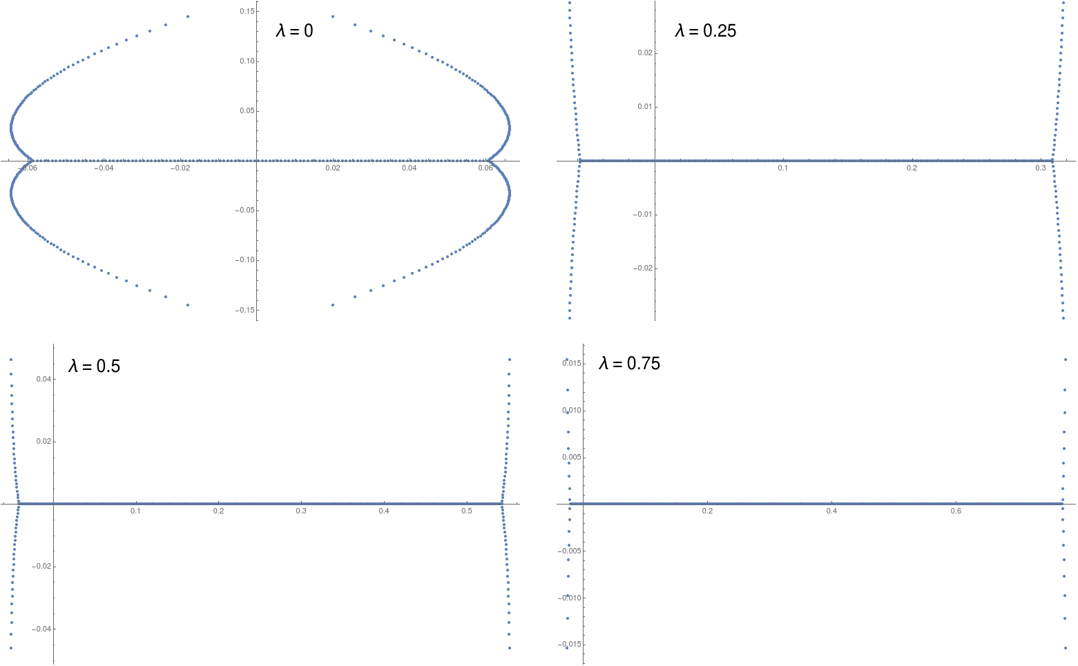
The two measures μ0\mu_{0} and μ1\mu_{1} can be viewed as two extreme points of the asymptotic zero distribution μλ\mu_{\lambda} of the polynomials

z↦Bn(1−λ+λ​n)​(n​z),z\mapsto B_{n}^{(1-\lambda+\lambda n)}(nz), (63)

where λ∈[0,1]\lambda\in[0,1]. The order of the above generalized Bernoulli polynomial is nothing but the convex combination of 11 and nn. The measures μλ\mu_{\lambda} seem to be absolutely continuous and continuously dependent on λ\lambda. An interesting research problem would be to describe the support (the zero attractor) as well as the density of μλ\mu_{\lambda} for λ∈(0,1)\lambda\in(0,1). For an illustration of approximate supports of μλ\mu_{\lambda} for several values of λ\lambda, see Figure 2.

Refer to caption
Figure 2. Plots of the zeros of the polynomials (63) in the complex plane for n=500n=500 and λ∈{0,1/4,1/2,3/4}\lambda\in\{0,1/4,1/2,3/4\} illustrating how the zero attractor of the Bernoulli polynomials (case OPENλ=0)\lambda=0) deforms into the interval [0,1][0,1] (case λ=1\lambda=1) as λ\lambda changes from 00 to 11.

3.5. Open problem: A uniform asymptotic expansion of Bn(n)​(n​x)B_{n}^{(n)}(nx) for all x∈[0,1]x\in[0,1]

As pointed out by an anonymous referee, it would be also an interesting open problem to find an asymptotic approximation for Bn(n)​(n​x)B_{n}^{(n)}(nx) that holds uniformly for x∈[0,1]x\in[0,1]. Such approximation, if exists, should involve some interesting special functions reflecting the behavior of Bn(n)​(n​x)B_{n}^{(n)}(nx) near the edge points x=0x=0 and x=1x=1.

Acknowledgement

The author is grateful to two referees for careful reports that improved the paper. Further, the author acknowledges financial support by the Ministry of Education, Youth and Sports of the Czech Republic project no. CZ.02.1.01/0.0/0.0/16_019/0000778.

References

  • [1] Blagouchine, I. V. A note on some recent results for the Bernoulli numbers of the second kind. J. Integer Seq. 20, 3 (2017), Art. 17.3.8, 7.
  • [2] Blagouchine, I. V. Three notes on Ser’s and Hasse’s representations for the zeta-functions. Integers 18A (2018), Paper No. A3, 45.
  • [3] Boyer, R., and Goh, W. M. Y. On the zero attractor of the Euler polynomials. Adv. in Appl. Math. 38, 1 (2007), 97–132.
  • [4] Brillhart, J. On the Euler and Bernoulli polynomials. J. Reine Angew. Math. 234 (1969), 45–64.
  • [5] Carlitz, L. A note on Bernoulli and Euler polynomials of the second kind. Scripta Math. 25 (1961), 323–330.
  • [6] Conway, J. B. Functions of one complex variable, second ed., vol. 11 of Graduate Texts in Mathematics. Springer-Verlag, New York-Berlin, 1978.
  • [7] Delange, H. Sur les zéros réels des polynômes de Bernoulli. C. R. Acad. Sci. Paris Sér. I Math. 303, 12 (1986), 539–542.
  • [8] Delange, H. Sur les zéros réels des polynômes de Bernoulli. Ann. Inst. Fourier (Grenoble) 41, 2 (1991), 267–309.
  • [9] Dilcher, K. Asymptotic behaviour of Bernoulli, Euler, and generalized Bernoulli polynomials. J. Approx. Theory 49, 4 (1987), 321–330.
  • [10] Dilcher, K. On multiple zeros of Bernoulli polynomials. Acta Arith. 134, 2 (2008), 149–155.
  • [11] NIST Digital Library of Mathematical Functions. http://dlmf.nist.gov/, Release 1.0.17 of 2017-12-22. F. W. J. Olver, A. B. Olde Daalhuis, D. W. Lozier, B. I. Schneider, R. F. Boisvert, C. W. Clark, B. R. Miller and B. V. Saunders, eds.
  • [12] Edwards, R., and Leeming, D. J. The exact number of real roots of the Bernoulli polynomials. J. Approx. Theory 164, 5 (2012), 754–775.
  • [13] Efimov, A. I. The asymptotics for the number of real roots of the Bernoulli polynomials. Forum Math. 20, 2 (2008), 387–393.
  • [14] Guo, B.-N., Mező, I., and Qi, F. An explicit formula for Bernoulli polynomials in terms of rr-Stirling numbers of the second kind. Rocky Mountain J. Math. 46, 6 (2016), 1919–1923.
  • [15] Gupta, S., and Prabhakar, T. R. Bernoulli polynomials of the second kind and general order. Indian J. Pure Appl. Math. 11, 10 (1980), 1361–1368.
  • [16] Inkeri, K. The real roots of Bernoulli polynomials. Ann. Univ. Turku. Ser. A I 37 (1959), 20.
  • [17] Kim, T., Kwon, H. I., Lee, S. H., and Seo, J. J. A note on poly-Bernoulli numbers and polynomials of the second kind. Adv. Difference Equ. (2014), 2014:219, 6.
  • [18] Leeming, D. J. The real zeros of the Bernoulli polynomials. J. Approx. Theory 58, 2 (1989), 124–150.
  • [19] López, J. L., and Temme, N. M. Hermite polynomials in asymptotic representations of generalized Bernoulli, Euler, Bessel, and Buchholz polynomials. J. Math. Anal. Appl. 239, 2 (1999), 457–477.
  • [20] López, J. L., and Temme, N. M. Large degree asymptotics of generalized Bernoulli and Euler polynomials. J. Math. Anal. Appl. 363, 1 (2010), 197–208.
  • [21] Nemes, G. An asymptotic expansion for the Bernoulli numbers of the second kind. J. Integer Seq. 14, 4 (2011), Article 11.4.8, 6.
  • [22] Neuschel, T. A uniform version of Laplace’s method for contour integrals. Analysis (Munich) 32, 2 (2012), 121–135.
  • [23] Nörlund, N. E. Vorlesungen über Differenzenrechnung. Springer, Berlin, Germany, 1924. reprinted by Chelsea, Bronx, NY, USA, 1954.
  • [24] Nörlund, N. E. Sur les valeurs asymptotiques des nombres et des polynômes de Bernoulli. Rend. Circ. Mat. Palermo (2) 10 (1961), 27–44.
  • [25] Olver, F. W. J. Asymptotics and special functions. AKP Classics. A K Peters, Ltd., Wellesley, MA, 1997. Reprint of the 1974 original [Academic Press, New York; MR0435697 (55 # 8655)].
  • [26] Roman, S. The umbral calculus, vol. 111 of Pure and Applied Mathematics. Academic Press, Inc. [Harcourt Brace Jovanovich, Publishers], New York, 1984.
  • [27] Schröder, E. Bestimmung des infinitären Werthes des Integrals ∫01(u)n​𝑑u\int_{0}^{1}(u)_{n}du. Z. Math. Phys. 25 (1880), 106–117.
  • [28] Shapiro, B., and Štampach, F. Non-self-adjoint Toeplitz matrices whose principal submatrices have real spectrum. Constr. Approx. 49, 2 (2019), 191–226.
  • [29] Slavić, D. V. On coefficients of the Gauss-Encke formula. Univ. Beograd. Publ. Elektrotehn. Fak. Ser. Mat. Fiz., 498-541 (1975), 33–38.
  • [30] Srivastava, H. M., and Choi, J. Series associated with the zeta and related functions. Kluwer Academic Publishers, Dordrecht, 2001.
  • [31] Srivastava, H. M., and Todorov, P. G. An explicit formula for the generalized Bernoulli polynomials. J. Math. Anal. Appl. 130, 2 (1988), 509–513.
  • [32] Steffensen, J. F. On laplace’s and gauss’ summation-formulas. Scandinavian Actuarial Journal 1924, 1 (1924), 1–15.
  • [33] van Veen, S. C. Asymptotic expansion of the generalized Bernoulli numbers Bn(n−1)B_{n}^{(n-1)} for large values of n⁡(nCLOSEn(n integer). Nederl. Akad. Wetensch. Proc. Ser. A. 54 = Indagationes Math. 13 (1951), 335–341.
  • [34] Veselov, A. P., and Ward, J. P. On the real zeroes of the Hurwitz zeta-function and Bernoulli polynomials. J. Math. Anal. Appl. 305, 2 (2005), 712–721.
  • [35] Wong, R. Asymptotic approximations of integrals, vol. 34 of Classics in Applied Mathematics. Society for Industrial and Applied Mathematics (SIAM), Philadelphia, PA, 2001. Corrected reprint of the 1989 original.