跳到论文正文
W Papers独立论文阅读器 arXiv:2011.13772 论文正文 计算阅读时间 · 0%
引用这篇论文根据当前论文元数据生成,正式投稿前建议核对。


License: arXiv.org perpetual non-exclusive license
arXiv:2011.13772v5 [cs.LG] 21 Aug 2023

Gradient Descent for Deep Matrix Factorization:
Dynamics and Implicit Bias towards Low Rank

Hung-Hsu Chou Affiliation: Department of Mathematics, LMU Munich, Germany    Carsten Gieshoff Affiliation: Chair for Mathematics of Information Processing, RWTH Aachen University, Germany    Johannes Maly Affiliation: Department of Mathematics, LMU Munich, Germany    Holger Rauhut Affiliation: Department of Mathematics, LMU Munich, Germany
August 11, 2026
Abstract

In deep learning, it is common to use more network parameters than training points. In such scenario of over-parameterization, there are usually multiple networks that achieve zero training error so that the training algorithm induces an implicit bias on the computed solution. In practice, (stochastic) gradient descent tends to prefer solutions which generalize well, which provides a possible explanation of the success of deep learning. In this paper we analyze the dynamics of gradient descent in the simplified setting of linear networks and of an estimation problem. Although we are not in an overparameterized scenario, our analysis nevertheless provides insights into the phenomenon of implicit bias. In fact, we derive a rigorous analysis of the dynamics of vanilla gradient descent, and characterize the dynamical convergence of the spectrum. We are able to accurately locate time intervals where the effective rank of the iterates is close to the effective rank of a low-rank projection of the ground-truth matrix. In practice, those intervals can be used as criteria for early stopping if a certain regularity is desired. We also provide empirical evidence for implicit bias in more general scenarios, such as matrix sensing and random initialization. This suggests that deep learning prefers trajectories whose complexity (measured in terms of effective rank) is monotonically increasing, which we believe is a fundamental concept for the theoretical understanding of deep learning.

Keywords — Gradient Descent, Implicit Bias/Regularization, Matrix Factorization, Neural Networks

1 Introduction

Deep learning has become the standard machine learning technology in recent years, celebrating breakthroughs in many areas ranging from face recognition over medical imaging to autonomous driving. Despite all its successes it is still mysterious why deep learning works so well. Often deep neural networks have significantly more parameters than the number of examples used in training. As studied systematically via numerical experiments, for instance in [18, 22, 28], (stochastic) gradient descent usually results in zero training error so that the resulting neural networks interpolate the training samples exactly. Nevertheless and somewhat surprisingly, the trained deep networks generalize very well, although classical statistics would suggest that one is in a regime of overfitting. It was remarked already in [28] that the employed optimization algorithms induce an implicit bias towards certain solutions. Apparently, those solutions often behave very nicely in realistic situations. Providing an understanding of the nature of such implicit bias seems to be a key task for the development and understanding of deep learning in general. While a general theory for the implicit bias in deep learning seems presently out of reach, first theoretical works [2, 7, 11, 12, 23, 24] concentrate on linear networks and suggest that (stochastic) gradient descent converges to a linear network, i.e., a linear function described by a matrix, which is of low rank. Nevertheless, even for the linear case, the settings considered in these works are rather restrictive and many open questions remain.

In this article, we consider a matrix estimation problem, see (5) below, where the desired matrix W∈ℝn×nW~\in~\mathbb{R}^{n\times n} (describing the linear network) is factorized into NN matrices W1,…,WN∈ℝn×nW_{1},\ldots,W_{N}\in\mathbb{R}^{n\times n}. We provide a precise analysis of the dynamics of the gradient descent/flow for each of the individual matrices WjW_{j}, which are initialized by α​I\alpha I, for some suitable small constant α>0\alpha>0. We show that for desired rank LL and explicitly given time-intervals the time-dependent product matrix approximates very well the best rank LL approximation of the ground truth matrix. In this way, we provide another indication of the role of low rank in the study of implicit bias in deep learning. We are convinced that our proof methods can be extended to study this problem in more general scenarios.

Let us describe the setting of our article in more details. The archetype of deep networks is the so-called feed-forward neural network of NN layers, N≥1N\geq 1, defined as h:ℝn0→ℝnNh\colon\mathbb{R}^{n_{0}}\rightarrow\mathbb{R}^{n_{N}} with

h(x)=gN∘⋯∘g1(x),\displaystyle h(x)=g_{N}\circ\cdots\circ g_{1}(x), (1)

where the functions gk:ℝnk−1→ℝnkg_{k}\colon\mathbb{R}^{n_{k-1}}\rightarrow\mathbb{R}^{n_{k}} are of the form

gk​(x)=σ⁡(Wk​x+bk)\displaystyle g_{k}(x)=\sigma(W_{k}x+b_{k})

and model the NN layers. They are determined by weight matrices Wk∈ℝnk×nk−1W_{k}\in\mathbb{R}^{n_{k}\times n_{k-1}}, bias terms bk∈ℝnkb_{k}\in\mathbb{R}^{n_{k}} (which we for simplicity set to bk=0b_{k}=0 from here on), and an activation function σ:ℝ→ℝ\sigma\colon\mathbb{R}\rightarrow\mathbb{R} that is in general non-linear and acting component-wise. To guarantee good performance, both the weight matrices and the bias terms are design parameters that are optimized according to the concrete data and application. For a fixed activation function σ\sigma and given training data (xi,yi)i=1M(x_{i},y_{i})_{i=1}^{M}, where xi∈ℝn0x_{i}\in\mathbb{R}^{n_{0}} and yi∈ℝnNy_{i}\in\mathbb{R}^{n_{N}} model training input resp. output, the standard approach in supervised learning is to solve

minW1,…,WN⁡1M​∑i=1Mℒ⁡(h⁡(xi),yi),\displaystyle\min_{W_{1},...,W_{N}}\frac{1}{M}\sum_{i=1}^{M}\mathcal{L}(h(x_{i}),y_{i}), (2)

where ℒ:ℝnN×ℝnN→ℝ+={x∈ℝ:x≥0}\mathcal{L}\colon\mathbb{R}^{n_{N}}\times\mathbb{R}^{n_{N}}\rightarrow\mathbb{R}_{+}=\{x\in\mathbb{R}:x\geq 0\} is called loss function and should exhibit ”distance like” properties (a popular choice being the squared ℓ2\ell_{2}-norm). The number of free parameters commonly dominates the number of training samples. In this case, we speak of overparametrization.

The optimization problem (2) is normally solved via variants of (stochastic) gradient descent (using back propagation). As already described above, this often leads to decent solutions, even in the overparametrized setting and a recent research hypothesis claims an implicit bias of gradient descent towards low-complexity solutions – although no regularization term is added to (2). It was observed in [13, 25] that early stopping may produce beneficial solutions while omitting unfavorable local and global minima. Since (2) is hard to analyze in general due to the non-linear structure of (1), recent theoretical works concentrate on the simplified case of linear neural networks [1, 2, 3, 5, 9, 20], where σ⁡(x)=x\sigma(x)=x and bk=0b_{k}=0, i.e., (1) becomes

hLinear(x)=WN⋯W1x.\displaystyle h_{\text{Linear}}(x)=W_{N}\cdots W_{1}x. (3)

Choosing ℒ\mathcal{L} to be the quadratic loss, equation (2) then takes the more accessible shape

minW1,…,WN1M∑i=1M‖WN⋯W1xi−yi‖22.\displaystyle\min_{W_{1},...,W_{N}}\frac{1}{M}\sum_{i=1}^{M}\left\|W_{N}\cdots W_{1}x_{i}-y_{i}\right\|_{2}^{2}. (4)

This problem reminds of classical formulations of principal component analysis (PCA) in [26]. Indeed, if the samples x1,…,xMx_{1},\dots,x_{M} span the input space ℝn0\mathbb{R}^{n_{0}}, any minimizer of (4) has to satisfy WN⋯W1=YX†=:W^∈ℝnN×n0W_{N}\cdots W_{1}=YX^{\dagger}=:\widehat{W}\in\mathbb{R}^{n_{N}\times n_{0}}, where X∈ℝn0×MX\in\mathbb{R}^{n_{0}\times M} and Y∈ℝnN×MY\in\mathbb{R}^{n_{N}\times M} have columns xix_{i} and yiy_{i}, for i∈[M]i\in[M], and X†X^{\dagger} denotes the pseudo-inverse of XX. The set of minimizers of (4) thus equals the set of minimizers of the matrix factorization problem

minW1,…,WN∥WN⋯W1−W^∥F2\displaystyle\min_{W_{1},...,W_{N}}\big\|W_{N}\cdots W_{1}-\widehat{W}\big\|_{F}^{2} (5)

for W^=Y​X†\widehat{W}=YX^{\dagger}, where ‖⋅‖F\left\|\cdot\right\|_{F} denotes the Frobenius norm. Note that, although the trajectories of gradient descent on (4) and (5) do not agree in general, the iterates are biased towards similar low-dimensional structures. Indeed, the recent works [2, 8, 12, 20] point out that, when applied to factorized problems like (4), (5), or matrix sensing and initialized close to zero, gradient descent exhibits an implicit bias towards solutions of low-rank resp. low nuclear norm even if the architecture is not imposing any rank constraints on the solution, i.e., n0=n1=⋯=nN=n∈ℕn_{0}=n_{1}=\cdots=n_{N}=n\in\mathbb{N}. It was, moreover, observed that higher order factorizations W=WN⋯W1W=W_{N}\cdots W_{1} can strengthen the regularizing effect [2]. We are convinced that understanding this phenomenon in detail will also help to gain theoretical insights into the success of gradient descent in the general training model (2). Let us mention that the trajectories of gradient descent on (4) and (5) do not agree in general. We focus on (5) in this work to allow a tighter theoretical analysis. For similar reasons, we make the simplifying assumption that all the matrices WjW_{j} are initialized by a small constant times the identity matrix although random initializations are often used in practice. We plan to extend this case to more general initializations in future work.

Hence, we are interested in analyzing the discrete dynamics defined by

Wj​(k+1)\displaystyle W_{j}({k}+1) =Wj​(k)−η​∇Wjℒ​(W⁡(k))\displaystyle=W_{j}({k})-\eta\nabla_{W_{j}}\mathcal{L}(W({k})) (6)
Wj​(0)\displaystyle W_{j}(0) =α​W0,\displaystyle=\alpha W_{0}, (7)

for j∈[N]:={1,…,N}j\in[N]:=\left\{1,\dots,N\right\}, where

ℒ⁡(W)=12​‖W−W^‖F2with∇Wℒ​(W)=(W−W^),\displaystyle\mathcal{L}(W)=\frac{1}{2}\big\|W-\widehat{W}\big\|_{F}^{2}\quad\text{with}\quad\nabla_{W}\mathcal{L}(W)=(W-\widehat{W}), (8)

η>0\eta>0 is the step-size, W0W_{0} is some initialization matrix, and α>0\alpha>0 is assumed to be small. Note that the gradient of ℒ\mathcal{L} with respect to a single factor WjW_{j} is given by

∇Wjℒ(W)=(WN⋯Wj+1)⊤∇Wℒ(W)(Wj−1⋯W1)⊤.\displaystyle\nabla_{W_{j}}\mathcal{L}(W)=(W_{N}\cdots W_{j+1})^{\top}\nabla_{W}\mathcal{L}(W)(W_{j-1}\cdots W_{1})^{\top}. (9)

1.1 Contribution and Outline

Shallow (OPENN=2)N=2) Deep (N>2N>2)
Gradient descent [8], [20] Our work
Gradient flow [12, 11] Our work, [1, 2]
Table 1: Comparison of our work with related literature in terms of which method is analyzed and whether the analysis is restricted to shallow factorizations.
Initialization Ground-truth Model
Our work identity symmetric (5)
[8] aligned X​XTXX^{T} and XT​Y​YT​XX^{T}YY^{T}X almost commuting (4)
[1, 2] identity symmetric PSD matrix sensing with commuting measurements
[12, 11] identity symmetric PSD matrix sensing with commuting measurements
[20] orthogonal symmetric PSD matrix sensing
Table 2: Comparison of our work with related literature in terms of considered initialization, ground-truth, and training model. Aligned initialization under the training model (4) means that WN​(0)W_{N}(0) has the same singular vectors as Y​XTYX^{T} and W1​(0)W_{1}(0) has the same singular vectors as X​XTXX^{T}. Orthogonal initialization means that all Wj​(0)W_{j}(0) are orthogonal matrices. Note that PSD stands for positive semi-definite ground-truths.

In this paper, we provide a precise analysis of the dynamics in (6)-(7) and their underlying continuous counterparts, for W0=IW_{0}=I and symmetric ground-truths W^∈ℝn×n\widehat{W}\in\mathbb{R}^{n\times n}. Our analysis extends/generalizes the one started in [2, 9, 20], which consider more sophisticated training models than (5) but basically restrict themselves to the gradient flow and gradient descent with N=2N=2, cf. Tables 1 and 2. In particular, our contributions are the following.

  1. 1.

    We analyze the gradient descent dynamics for all N∈ℕN\in\mathbb{N} (rather than only for N=2N=2 or rather than restricting only to the gradient flow.)

  2. 2.

    We derive a sharp upper bound on the step size η\eta ensuring convergence, for all choices of α\alpha and NN.

  3. 3.

    We only assume symmetry of the ground-truth, which is considerably weaker than the often used assumption of positive semidefiniteness (PSD).

  4. 4.

    We prove that negative eigenvalues can only be recovered under a suitable perturbation of the initialization. This has not yet been discussed in the standard setting of identity initialization since the prior works [2, 9, 20] only consider positive semi-definite ground-truths, cf. Table 2.

Our main results consist of three central observations (note that we always use explicit constants in the statements).

I. Recovery of positive eigenvalues: Initializing with W0=IW_{0}=I, as done in [20] in a matrix sensing framework, the dynamics in (6)-(7) can solely recover non-negative eigenvalues of W^\widehat{W}. In addition, the following theorem provides a quantitative analysis that shows how fast eigenvalues of W^\widehat{W} are approximated depending on their magnitude and other model parameters like NN, η\eta, and α\alpha.

Theorem 1.1.

Let N≥2N\geq 2, α>0\alpha>0, ε>0\varepsilon>0. Let W^=V​Λ​V⊤∈ℝn×n\widehat{W}=V\Lambda V^{\top}\in\mathbb{R}^{n\times n} be an eigendecomposition of the symmetric matrix W^\widehat{W} with Λ=diag(λi:i∈[n])\Lambda=\mathrm{diag}(\lambda_{i}:i\in[n]). Consider W1​(k),…,WN​(k)∈ℝn×nW_{1}({k}),\ldots,W_{N}({k})\in\mathbb{R}^{n\times n} and W(k)=WN(k)⋯W1(k)W({k})=W_{N}({k})\cdots W_{1}({k}) defined by the gradient descent iteration (6) with loss function (8) and identical initialization (7). Define M=max⁡(α,‖W^‖1N)M=\max(\alpha,\|\widehat{W}\|^{\frac{1}{N}}). Suppose

0<η<1(3​N−2)​M2​N−2.0<\eta<\frac{1}{(3N-2)M^{2N-2}}. (10)

Then W⁡(k)W({k}) converges to V​Λ+​V⊤V\Lambda_{+}V^{\top} as k→∞k\to\infty, where Λ+=diag(max{λi,0}:i∈[n])\Lambda_{+}=\mathrm{diag}(\max\{\lambda_{i},0\}:i\in[n]). Moreover, the error E⁡(k)=(V⊤​W​(k)​V−Λ+)E({k})=(V^{\top}W({k})V-\Lambda_{+}) is a diagonal matrix, whose entries satisfy

|Ei​i​(k)|≤{ε​N​λi1−1N if ​λi>0,εN if ​λi≤0.|E_{ii}({k})|\leq\begin{cases}\varepsilon N\lambda_{i}^{1-\frac{1}{N}}&\mbox{ if }\lambda_{i}>0,\\ \varepsilon^{N}&\mbox{ if }\lambda_{i}\leq 0.\end{cases} (11)

for all k≥TNId​(λi,ε,α,η)k\geq T^{\operatorname{Id}}_{N}(\lambda_{i},\varepsilon,\alpha,\eta), where TNIdT^{\operatorname{Id}}_{N} is defined in (23) below.

The proof of Theorem 1.1 is given in Section 2.1.

Remark 1.2.

The exact form of TNIdT_{N}^{\text{Id}} involves some additional notation, which will be introduced later, see (23). Let us nevertheless give some simplified approximate expressions in the relevant case that N≥3N\geq 3, 0<εN≪λi≤λ10<\varepsilon^{N}\ll\lambda_{i}\leq\lambda_{1} and 0<αN≪λi0<\alpha^{N}\ll\lambda_{i}, so that the initial matrix W⁡(0)=αN​IdW(0)=\alpha^{N}{\operatorname{Id}} has small enough spectral norm compared to the ii-th eigenvalue of the ground truth, which in turn is larger than the desired accuracy εN\varepsilon^{N}. In this case M=‖W^‖1N=λ11NM=\|\widehat{W}\|^{\frac{1}{N}}=\lambda_{1}^{\frac{1}{N}} and we assume that

η=κN​λ12−2N\eta=\frac{\kappa}{N\lambda_{1}^{2-\frac{2}{N}}}

for some κ≤13\kappa\leq\frac{1}{3} so that (10) is satisfied. The quantity TNIdT^{\operatorname{Id}}_{N} then takes the form (the interested reader is referred to the more detailed derivation and discussion in Appendix A)

TNId​(λi,ε,α,η)=1κ⁡(N−2)​(λ1αN)1−2N​λ1λi+𝒪⁡(log⁡(1/ε)),T^{\text{Id}}_{N}(\lambda_{i},\varepsilon,\alpha,\eta)=\frac{1}{\kappa(N-2)}\left(\frac{\lambda_{1}}{\alpha^{N}}\right)^{1-\frac{2}{N}}\frac{\lambda_{1}}{\lambda_{i}}+\mathcal{O}\big(\log(1/\varepsilon)\big), (12)

where we ignore the additional term sN​(λi,α)s_{N}(\lambda_{i},\alpha) appearing in (23) since it is neglectable for small κ\kappa and large NN (and probably resembles a proof artefact). As (12) shows, TNIdT^{\text{Id}}_{N} consists of two main terms. One depends on the ratio between λi\lambda_{i} and λ1\lambda_{1} and one on the desired accuracy ε\varepsilon. TNIdT^{\text{Id}}_{N} increases for smaller λi\lambda_{i} and ε\varepsilon.

Refer to caption
(a) Convergence of eigenvalues with identical initialization.
Refer to caption
(b) Convergence of eigenvalues with perturbed identical initialization.
Figure 1: Depicted is a comparison of gradient descent dynamics for different types of initialization. Depicted is the evolution of the entries (V⊤​W​V)i​i(V^{\top}WV)_{ii}, where VV diagonalizes W^\widehat{W}. In the case of identical initialization, only positive eigenvalues can be recovered, while in the case of perturbed identical initialization, the full spectrum is recovered. In addition, the recovering rate is positively correlated with the magnitude of eigenvalues. Here N=3N=3, α=10−1\alpha=10^{-1}, β=α2\beta=\frac{\alpha}{2}, and η=10−3\eta=10^{-3}.
Refer to caption
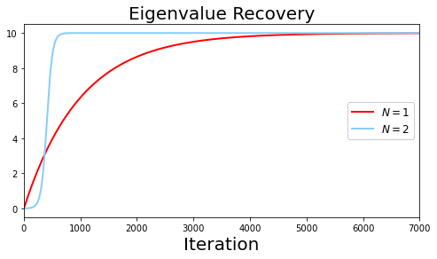
(a) The dynamics between N=1N=1 and N=2N=2 are quite different, in the sense that the transition for N=2N=2 is more concentrated.
Refer to caption
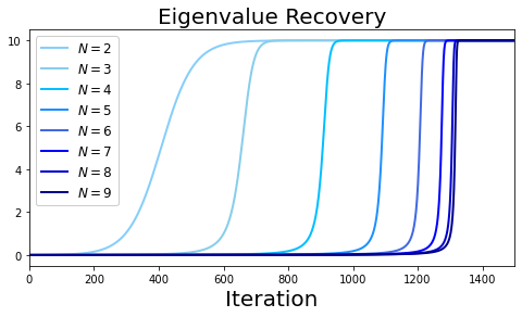
(b) For N≥2N\geq 2, the dynamics are more similar. As NN increases, the recovery rate becomes slower initially, but sharper once the transition occurs.
Figure 2: Depicted is a comparison of eigenvalue recovery rate for different number of layers NN with identical initialization. To make the comparison fair we fixed αN=3⋅10−3\alpha^{N}=3\cdot 10^{-3}. Here λ=10\lambda=10 and η=10−3\eta=10^{-3}.

II. Recovery of arbitrary eigenvalues: Perturbing the initialization slightly, i.e., setting

Wj​(0)={(α−β)​I if ​j=1α​I otherwise,W_{j}(0)=\begin{cases}(\alpha-\beta)I&\text{ if }j=1\\ \alpha I&\text{ otherwise},\end{cases} (13)

allows the dynamics in (6) to recover the whole spectrum of W^\widehat{W}, cf. Figure 1(b). This suggests that the spectral cut-off observed in Theorem 1.1 is a pathological case and thus hardly observed in practice. As before, the following theorem also quantifies the approximation rates of eigenvalues of W^\widehat{W} in terms of their magnitude, their sign, NN, η\eta, α\alpha, and β\beta.

Theorem 1.3.

Let N≥2N\geq 2 and let W^=V​Λ​V⊤∈ℝn×n\widehat{W}=V\Lambda V^{\top}\in\mathbb{R}^{n\times n} be an eigendecomposition of the symmetric matrix W^\widehat{W} with Λ=diag(λi:i∈[n])\Lambda=\mathrm{diag}(\lambda_{i}:i\in[n]). Consider W1​(k),…,WN​(k)∈ℝn×nW_{1}({k}),\ldots,W_{N}({k})\in\mathbb{R}^{n\times n} and W(k)=WN(k)⋯W1(k)W({k})=W_{N}({k})\cdots W_{1}({k}) defined by the gradient descent iteration defined in (6) with loss function (8) and perturbed identical initialization (13), where 0<βc−1<α0<\frac{\beta}{c-1}<\alpha, and c∈(1,2)c\in(1,2) is the maximal real solution to the polynomial equation 1=(c−1)​cN−11=(c-1)c^{N-1}. Define M=max⁡(α,‖W^‖1N)M=\max(\alpha,\|\widehat{W}\|^{\frac{1}{N}}). If

0<η<19​N​(c​M)2​N−2,0<\eta<\frac{1}{9N(cM)^{2N-2}}, (14)

then W⁡(k)W({k}) converges to W^\widehat{W}. Moreover, the error E⁡(k)=(V⊤​W​(k)​V−Λ)E({k})=(V^{\top}W({k})V-\Lambda) is a diagonal matrix, whose entries satisfy

|Ei​i(k)|≤{ε​N​|λi|1−1N for all ​k≥TNP​(λi,ε,α,β,η) if ​|λi|≥αN,αN for all ​k∈ℕ0 if ​0≤λi<αN,2​αN for all ​k∈ℕ0 if −αN≤λi<0.|E_{ii}({k})|\leq\left\{\begin{aligned} \varepsilon N|\lambda_{i}|^{1-\frac{1}{N}}&\mbox{ for all }{k}\geq T^{\operatorname{P}}_{N}(\lambda_{i},\varepsilon,\alpha,\beta,\eta)&\text{ if }|\lambda_{i}|\geq\alpha^{N},\\ \alpha^{N}\phantom{BLA}&\mbox{ for all }{k}\in\mathbb{N}_{0}&\text{ if }0\leq\lambda_{i}<\alpha^{N},\\ 2\alpha^{N}\phantom{BLA}&\mbox{ for all }{k}\in\mathbb{N}_{0}&\text{ if }-\alpha^{N}\leq\lambda_{i}<0.\\ \end{aligned}\right. (15)

for all ε∈(0,|λi|1N)\varepsilon\in(0,|\lambda_{i}|^{\frac{1}{N}}), and

TNP​(λ,ε,α,β,η):={TNId​(λ,ε,α,η) if ​λ≥αN,TNId​(|λ|,ε,β,η)+αη​(9​N−2​(c−1)9​N​β​|λ|1N)N−1​(|λ|1N−βc−1) if ​λ≤−αN,T_{N}^{\operatorname{P}}(\lambda,\varepsilon,\alpha,\beta,\eta):=\begin{cases}T_{N}^{{\operatorname{Id}}}(\lambda,\varepsilon,\alpha,\eta)&\text{ if }\lambda\geq\alpha^{N},\\ \displaystyle{T^{\operatorname{Id}}_{N}\left(|\lambda|,\varepsilon,\beta,\eta\right)+\frac{\alpha}{\eta\left(\frac{9N-2(c-1)}{9N}\beta|\lambda|^{\frac{1}{N}}\right)^{N-1}\left(|\lambda|^{\frac{1}{N}}-\frac{\beta}{c-1}\right)}}&\text{ if }\lambda\leq-\alpha^{N},\end{cases} (16)

where TNIdT^{{\operatorname{Id}}}_{N} is defined in (23).

The proof of Theorem 1.3 is given in Section 2.2.

Remark 1.4.

Apart from again providing precise bounds on the number of iterations sufficient to obtain a predefined approximation accuracy, Theorem 1.3 is instructive in pointing out two qualitatively different regimes of the gradient descent dynamics. If λi\lambda_{i} is positive, the dynamics behave as in Theorem 1.1. If λi\lambda_{i} is negative, however, gradient descent first approximates (λi)+=0(\lambda_{i})_{+}=0 up to perturbation level β\beta. As soon as this level is reached, the dynamics force the ii-th eigenvalue of W1W_{1} to become negative while all others remain positive, as illustrated in Figure 1 and Figure 5 below. Afterwards the sign does not change and hence the negative eigenvalue is recovered.
Interestingly enough, in practice this phenomenon may also happen when running simulations with identical initialization. Although in theory the eigenvalues of W⁡(k)W(k) should remain non-negative, it is possible that the ii-th eigenvalue of some factor Wj​(k)W_{j}(k), which corresponds to a negative ground-truth eigenvalue, becomes negative due to numerical errors, i.e., when it reaches machine precision. As a consequence the ii-th eigenvalue of W⁡(k)W(k) becomes negative and converges to the ground-truth eigenvalue.
Note that the upper bound on η\eta in (14) decays in NN like Ω⁡(N−3)\Omega(N^{-3}) if α<1\alpha<1. This can be seen as follows: the defining equation of cc, which can be written as cN−cN−1=1c^{N}-c^{N-1}=1, implies that cℓ−cℓ−1≤1c^{\ell}-c^{\ell-1}\leq 1, for any ℓ=1,…,N\ell=1,\dots,N since c>1c>1. Hence,

cN−1=∑ℓ=1N(cℓ−cℓ−1)≤N,c^{N}-1=\sum_{\ell=1}^{N}(c^{\ell}-c^{\ell-1})\leq N,

such that c2​N−2≤c2​N≤(N+1)2c^{2N-2}\leq c^{2N}\leq(N+1)^{2}. Consequently, we obtain for α<1\alpha<1 that

19​N​(c​M)2​N−2≥19​N​(N+1)2​max⁡{1,‖W^‖2​N−2N}=Ω⁡(N−3).\frac{1}{9N(cM)^{2N-2}}\geq\frac{1}{9N(N+1)^{2}\max\{1,\|\widehat{W}\|^{\frac{2N-2}{N}}\}}=\Omega(N^{-3}).

Let us finally mention that the condition 0<βc−1<α0<\frac{\beta}{c-1}<\alpha is used to simplify parts of the argument. Numerical simulations suggest that it is an artifact of the proof ; 0<β<α0<\beta<\alpha is empirically sufficient.

III. Implicit bias towards low-rank: Theorems 1.1 and 1.3 suggest an implicit rank regularization of the gradient descent iterates W⁡(k)W({k}) if we stop at some appropriate finite kk, since dominant eigenvalues will be approximated faster than the rest of the spectrum. The discussion in Section 3 — in particular, Theorems 3.1 (gradient flow, N=2N=2) and 3.5 (gradient descent, N≥2N\geq 2) — makes this precise by showing that the effective rank (a generalized notion of rank) of the iterates W⁡(k)W({k}) first drops to one and then monotonously increases, plateauing on the effective rank levels of various low-rank approximations of W^\widehat{W}, cf. Figure 3. Theorems 3.1 and 3.5 explicitly characterize the time intervals during which the effective rank of W⁡(k)W({k}) remains approximately constant.

Refer to caption
Refer to caption
Figure 3: Dynamics of gradient descent (6)-(7) with N=2N=2, n=200n=200, α=10−2\alpha=10^{-2}, η=10−2\eta=10^{-2}. The matrix W^∈ℝn×n\widehat{W}\in\mathbb{R}^{n\times n} is symmetric of rank 33 with nonzero eigenvalues (λ1,λ2,λ3)=(10,5,1)(\lambda_{1},\lambda_{2},\lambda_{3})=(10,5,1). The shaded regions are the predictions of Theorem 3.1 on where the best rank LL approximation W^L\widehat{W}_{L} of W^\widehat{W} lies. Remarkably, those predictions correspond to the plateaus of gradient descent during training. The effective rank is defined as r⁡(W)=‖W‖∗/‖W‖r(W)=\|W\|_{*}/\|W\|, and all other parameters are chosen such that the prediction error (the upper bound in Theorem 3.1) is less than 10−110^{-1}.

In addition to those highlights, we provide numerical evidence supporting the theory and simulations in more general settings suggesting that our observations are not restricted to matrix factorization with symmetric ground truths. The organization of the paper is as follows: Section 2 contains the core analysis including a quantitative description of the dynamics in (6)-(7), both for the identical and the perturbed initialization. Building upon those results, Section 3 then deduces an implicit low-rank bias of gradient descent and compares theoretical predictions to actual numerical outcomes. Finally, we present in Section 4 additional numerical simulations in more general settings and discuss future work in Section 5.

1.2 Related Work

Linear multilayer neural networks and related optimization problems have been investigated in several works [1, 2, 3, 4, 7, 17, 20, 23]. In particular, it has been shown in [3] (extending [1, 2, 17]) that the gradient flow minimizing L(W1,…,WN)=12∥Y−WN⋯W1X∥F2L(W_{1},\ldots,W_{N})=\frac{1}{2}\|Y-W_{N}\cdots W_{1}X\|_{F}^{2}, i.e., learning deep linear networks, converges to a global minimizer for almost all initializations.

In [20] the authors consider the problem of recovering a symmetric, positive matrix XX of low rank from incomplete linear measurements y=𝒜⁡(X)y=\mathcal{A}(X). They are able to show that gradient descent on the factorized problem L⁡(W1)=12​‖y−𝒜⁡(W1​W1T)‖22L(W_{1})=\frac{1}{2}\|y-\mathcal{A}(W_{1}W^{T}_{1})\|_{2}^{2} converges to the ground truth if a restricted isometry assumption holds for 𝒜\mathcal{A}. While this seems to suggest a bias of gradient descent towards low-rank solutions, the conclusion is questionable because restricting the linear system y=𝒜⁡(W)y=\mathcal{A}(W) to positive semidefinite matrices WW often means that XX is the unique solution if y=𝒜⁡(X)y=\mathcal{A}(X) for a low rank matrix XX [7, 16].

It was observed empirically in a number of works, see e.g. [18, 22, 28], that training deep (nonlinear) overparameterized neural networks via (stochastic) gradient descent imposes an implicit bias towards networks that generalize well on unseen data. In fact, it came as a surprise that increasing the number of parameters may decrease the generalization error despite the fact that the training error is always zero. First works towards a theoretical explanation of this phenomenon include [2, 8, 7, 11, 12, 21, 23, 24]. As a first step, most of these works concentrate on linear networks. In [24, 11] the authors study classification problems and convolution networks. In particular, they show for gradient descent an implicit bias towards filters whose Fourier transform minimizes the ℓp\ell_{p}-norm, where p=2/Np=2/N (assuming that the loss function converges to zero for the gradient descent iterates). Matrix sensing problems are studied in [2, 12], where the authors concentrate on recovering a matrix X∈ℝn×nX\in\mathbb{R}^{n\times n} from linear measurements yi=𝒜​(X)i=tr​(AiT​X)y_{i}=\mathcal{A}(X)_{i}=\text{tr}(A_{i}^{T}X), i=1,…,mi=1,\ldots,m via gradient descent on the functional L^(W1,…,WN)=L(WN⋯W1)\widehat{L}(W_{1},\ldots,W_{N})=L(W_{N}\cdots W_{1}) with L⁡(W)=12​‖y−𝒜⁡(W)‖22L(W)=\frac{1}{2}\|y-\mathcal{A}(W)\|_{2}^{2} where Wj∈ℝn×nW_{j}\in\mathbb{R}^{n\times n}. Assuming that the measurement matrices AiA_{i} commute and XX is positive semidefinite these works show that if L⁡(W1​(k),…,WN​(k))→0L(W_{1}(k),\ldots,W_{N}(k))\to 0 as k→∞k\to\infty, then the limit W∞=limk→∞WN(k)⋯W1(k)W_{\infty}=\lim_{k\to\infty}W_{N}(k)\cdots W_{1}(k) minimizes the nuclear norm ‖W‖∗\|W\|_{*} among all positive semidefinite matrices WW satisfying y=𝒜⁡(W)y=\mathcal{A}(W). Whereas this is interesting, the restriction to commuting measurements and positive semidefinite ground truth seems very limiting. In particular, there may be at most nn linearly independent commuting measurement matrices AiA_{i} (usually one requires at least C​r​nCrn measurements to recover a matrix of rank nn) while the restriction to positive semidefinite matrices may result in uniqueness of the solution to y=𝒜⁡(W)y=\mathcal{A}(W), see also [7]. The article [23] indicates that implicit bias of gradient descent in deep matrix factorization may not be explainable by a norm (such as the nuclear norm) but rather via low rank. Our contribution seems to support this conjecture, but rigorously showing it for matrix recovery is still open. Only shortly before finishing our manuscript, we became aware of [9], which is probably conceptually closest to our work. The authors study the gradient flow and gradient descent dynamics in the same setting as we do and focus on the question under which choices of α\alpha the dynamics of pairwise different eigenvalues of the product WN⋯W1W_{N}\cdots W_{1} are distinguishable. Whereas parts of our technical results appeared in less general form in [9] before, cf. Section 2.1, our proof techniques and main results are fundamentally different. For further discussion on [9], we refer the reader to Section 3.3.

Early stopping of gradient descent in deep learning has been investigated in a number of contributions, see e.g. [5, 15, 27]. It may be interpreted as bias-variance trade-off [27]. In the context of neural tangent kernels, [15] shows that when the width of network becomes infinite, the convergence rate of gradient flow is faster for eigenspaces with larger eigenvalues. Hence, early stopping may seem appealing for applications where only few major features are required. In fact, early stopping is intertwined with the idea of implicit bias, as we will discuss later in our paper.

1.3 Notation

We abbreviate [n]:={1,…​n}[n]:=\left\{1,...n\right\}. We denote matrices by uppercase letters and scalars by lowercase letters. Norms that frequently appear are the operator norm (spectral norm) ‖A‖=sup‖x‖2=1‖A​x‖2\|A\|=\sup_{\|x\|_{2}=1}\|Ax\|_{2}, the Frobenius norm ‖A‖F=(∑j,k|Aj,k|2)1/2=tr​(AT​A)\|A\|_{F}=(\sum_{j,k}|A_{j,k}|^{2})^{1/2}=\sqrt{\text{tr}(A^{T}A)}, and the nuclear norm ∥⋅∥∗=∑jσ(A)j\|\cdot\|_{*}=\sum_{j}\sigma(A)_{j}, where σ​(A)j\sigma(A)_{j} are the singular values of AA. Throughout the paper, α\alpha represents the initialization, η\eta the step size, and NN the depth of the matrix factorization. For a real number aa, we denote a+=max⁡{0,a}a_{+}=\max\{0,a\}.

2 The Dynamics of Gradient Descent

The goal of this section is to derive precise bounds on the full trajectory of the gradient descent iterations W⁡(k)W({k}) defined in (6) for the quadratic loss function (8) where W^\widehat{W} is assumed to be a symmetric ground truth matrix. We first choose a small positive multiple of the identity as initialization of all factor matrices. However, we will see that we cannot recover negative eigenvalues of W^\widehat{W} with such initialization. To mend this, we will consider then a slightly modified initialization, which guarantees recovery of the ground truth W^\widehat{W} in the limit as k→∞{k}\to\infty, and characterize also the dynamics in this case.

2.1 Identical Initialization

We start by observing that the dynamics of the different eigenvalues decouple when initializing with the same multiple of the identity matrix. A similar result and proof has already appeared for the underlying gradient flow in [9, Section E.1].

Lemma 2.1.

Let (Wj​(k))j=1N(W_{j}({k}))_{j=1}^{N} be the solution to the gradient descent (6) with identical initialization (7) and let W^=V​Λ​VT\widehat{W}=V\Lambda V^{T} be an eigenvalue decomposition of the symmetric ground truth matrix (where VV is orthogonal). Then the matrices Dj​(k):=V⊤​Wj​(k)​VD_{j}({k}):=V^{\top}W_{j}({k})V are real, diagonal and identical, i.e., Dj​(k)=D​(k)D_{j}({k})=D({k}) for all jj for some D⁡(k)D({k}), and follow the dynamics

D⁡(k+1)=D⁡(k)−η​D​(k)N−1​(D​(k)N−Λ),k∈ℕ0.D({k}+1)=D({k})-\eta D({k})^{N-1}(D({k})^{N}-\Lambda),\quad k\in\mathbb{N}_{0}. (17)
Proof.

Let D⁡(0)=α​ID(0)=\alpha I and define D⁡(k)D({k}) for k∈ℕ{k}\in\mathbb{N} recursively via (17). We prove the claim that the matrices Dj​(k)D_{j}({k}) are real, diagonal and that Dj​(k)=D​(k)D_{j}({k})=D({k}) for all jj by induction. For k=0k=0 this is clearly true since Wj​(0)=α​IW_{j}(0)=\alpha I. Now suppose this claim holds for some k∈ℕ0{k}\in\mathbb{N}_{0}. Then by (9), we have, for all j=1,…,Nj=1,\ldots,N and k∈ℕ{k}\in\mathbb{N},

Wj​(k+1)\displaystyle W_{j}({k}+1) =Wj(k)−η(WN(k)⋯Wj+1(k))⊤(W(k)−W^)(Wj−1(k)⋯W1(k))⊤\displaystyle=W_{j}({k})-\eta(W_{N}({k})\cdots W_{j+1}({k}))^{\top}(W({k})-\widehat{W})(W_{j-1}({k})\cdots W_{1}({k}))^{\top}
=V​D​(k)​V⊤−η​(V​D​(k)j−1​V⊤)⊤​V​(D​(k)N−Λ)​V⊤​(V​D​(k)N−j​V⊤)⊤\displaystyle=VD({k})V^{\top}-\eta(VD({k})^{j-1}V^{\top})^{\top}V(D({k})^{N}-\Lambda)V^{\top}(VD({k})^{N-j}V^{\top})^{\top}
=V⁡[D⁡(k)−η​D​(k)N−1​(D​(k)N−Λ)]​V⊤=V​D​(k+1)​V⊤.\displaystyle=V[D({k})-\eta D({k})^{N-1}(D({k})^{N}-\Lambda)]V^{\top}=VD({k}+1)V^{\top}.

By orthogonality of VV this shows that Dj​(k+1)=D⁡(k+1)D_{j}(k+1)=D(k+1) so that the induction step is completed. ∎

Due to the previous decoupling lemma it suffices to analyze the dynamics of each diagonal entry of D⁡(k)D({k}) separately. Denoting by λ\lambda an eigenvalue of the ground truth matrix W^\widehat{W} the corresponding diagonal element d⁡(k)d({k}) of D⁡(k)D({k}) evolves according to the equation

d⁡(k+1)=d⁡(k)−η​d​(k)N−1​(d​(k)N−λ),d⁡(0)=α>0.d({k}+1)=d({k})-\eta d({k})^{N-1}(d({k})^{N}-\lambda),\quad d(0)=\alpha>0. (18)

The following lemma describes the convergence of dd in (18). It extends [9, Lemma 1] to negative choices of λ\lambda and to the case λ≤α\lambda\leq\alpha. Note that the proof is fundamentally different from the one presented in [9].

Lemma 2.2.

Let dd be the solution of (18) for some λ∈ℝ\lambda\in{\mathbb{R}} and α>0\alpha>0.

  • •

    If N=1N=1 and η∈(0,1)\eta\in(0,1), then dd converges to λ\lambda linearly, i.e.,

    |d⁡(k)−λ|≤(1−η)k​|α−λ| for all ​k∈ℕ.|d({k})-\lambda|\leq(1-\eta)^{k}|\alpha-\lambda|\quad\mbox{ for all }{k}\in\mathbb{N}.
  • •

    If N≥2N\geq 2 and

    0<η<{(N​max⁡{α,|λ|1N}2​N−2)−1 if ​λ>0,α−2​N+2 if ​λ≤0​ and ​α≥|λ|1N,((3​N−2)​|λ|2−2N)−1 if ​λ<0​ and ​0<α<|λ|1N,\displaystyle 0<\eta<\begin{cases}\left(N\max\left\{\alpha,|\lambda|^{\frac{1}{N}}\right\}^{2N-2}\right)^{-1}&\mbox{ if }\lambda>0,\\ \alpha^{-2N+2}&\mbox{ if }\lambda\leq 0\mbox{ \rm{and} }\alpha\geq|\lambda|^{\frac{1}{N}},\\ \left((3N-2)|\lambda|^{2-\frac{2}{N}}\right)^{-1}&\mbox{ if }\lambda<0\mbox{ \rm{and} }0<\alpha<|\lambda|^{\frac{1}{N}},\\ \end{cases}

    then limk→∞d⁡(k)=λ+1N=max⁡{λ,0}1N\lim_{{k}\to\infty}d({k})=\lambda_{+}^{\frac{1}{N}}=\max\{\lambda,0\}^{\frac{1}{N}}. Moreover, the error |d​(k)N−λ+||d({k})^{N}-\lambda_{+}| is monotonically decreasing and, for all k≥0{k}\geq 0, one has that d⁡(k)∈[α,λ1N]d({k})\in[\alpha,\lambda^{\frac{1}{N}}] if λ≥αN\lambda\geq\alpha^{N}, and d⁡(k)∈[λ+1N,α]d({k})\in[\lambda_{+}^{\frac{1}{N}},\alpha] if λ<αN\lambda<\alpha^{N}.

Remark 2.3.

Note that the proof of Lemma 2.2 shows that the sequence d⁡(k)d({k}) is monotonically increasing for λ>α\lambda>\alpha and monotonically decreasing for λ<α\lambda<\alpha. We will repeatedly make use of this observation in the following.

Proof.

For N=1N=1 the computation is straight-forward and follows by induction. For N≥2N\geq 2 we need to make a case distinction with four cases that depend on the sign and the magnitude of λ\lambda. This is due to the fact that the sign of λ\lambda determines the limit of dd, while the magnitude of λ\lambda determines whether dd is increasing or decreasing in time.

Let N≥2N\geq 2. Before diving into the case distinction, let us define, for |λ|1N>α|\lambda|^{\frac{1}{N}}>\alpha, the function

g⁡(x)=x−η​xN−1​(xN−λ)g(x)=x-\eta x^{N-1}(x^{N}-\lambda)

and observe that d⁡(k+1)=g⁡(d⁡(k))d({k}+1)=g(d({k})). For x∈[0,|λ|1N]x\in[0,|\lambda|^{\frac{1}{N}}], z=x/|λ|1/N∈[0,1]z=x/|\lambda|^{1/N}\in[0,1] and σ=sign⁡(λ)\sigma=\operatorname{sign}(\lambda) its derivative satisfies

g′​(x)\displaystyle g^{\prime}(x) =1−η⁡((N−1)​xN−2​(xN−λ)+N​x2​N−2)\displaystyle=1-\eta((N-1)x^{N-2}(x^{N}-\lambda)+Nx^{2N-2})
=1−η​|λ|2−2N​((N−1)​zN−2​(zN−σ)+N​z2​N−2)\displaystyle=1-\eta|\lambda|^{2-\frac{2}{N}}\left((N-1)z^{N-2}(z^{N}-\sigma)+Nz^{2N-2}\right)
≥{1−η​|λ|2−2N​N if ​λ>0,1−η​|λ|2−2N​(3​N−2) if ​λ<0,\displaystyle\geq\left\{\begin{array}[]{ll}1-\eta|\lambda|^{2-\frac{2}{N}}N&\mbox{ if }\lambda>0,\\ 1-\eta|\lambda|^{2-\frac{2}{N}}(3N-2)&\mbox{ if }\lambda<0,\end{array}\right.

where we used that z∈[0,1]z\in[0,1]. By the assumption on η\eta it follows that g′​(x)≥0g^{\prime}(x)\geq 0 for all x∈[0,|λ|1N]x\in[0,|\lambda|^{\frac{1}{N}}] and, hence, gg is monotonically increasing on that interval. We can now distinguish the four cases defined by λ≥0\lambda\geq 0/λ<0\lambda<0 and |λ|1N>α|\lambda|^{\frac{1}{N}}>\alpha/|λ|1N≤α|\lambda|^{\frac{1}{N}}\leq\alpha.

For λ>0\lambda>0 and |λ|1N>α|\lambda|^{\frac{1}{N}}>\alpha, gg has its fixed points at 00 and λ1N\lambda^{\frac{1}{N}} so that by monotonicity gg maps the interval [0,λ1N][0,\lambda^{\frac{1}{N}}] to itself. Hence, λ1N≥g⁡(x)>x\lambda^{\frac{1}{N}}\geq g(x)>x for all x∈(0,λ1N)x\in(0,\lambda^{\frac{1}{N}}) so that λ1N≥d⁡(k+1)>d⁡(k)\lambda^{\frac{1}{N}}\geq d({k}+1)>d({k}) for all k∈ℕ{k}\in{\mathbb{N}}. This means that the error |d​(k)N−λ||d({k})^{N}-\lambda| is monotonically decreasing. Hence, {d⁡(k)}k≥0\{d({k})\}_{{k}\geq 0} is an increasing bounded sequence. By the monotone convergence theorem, it converges to the unique fixed point λ1N\lambda^{\frac{1}{N}} of gg on [α,λ1/N][\alpha,\lambda^{1/N}].

For λ<0\lambda<0 and |λ|1N>α|\lambda|^{\frac{1}{N}}>\alpha, since gg is monotonically increasing on [0,|λ|1N][0,|\lambda|^{\frac{1}{N}}] and g⁡(0)=0g(0)=0 we have g⁡(x)≥0g(x)\geq 0 for all [0,|λ|1N][0,|\lambda|^{\frac{1}{N}}]. Note that g⁡(x)<xg(x)<x if λ≤0\lambda\leq 0 and x>0x>0. Since d⁡(0)=α>0d(0)=\alpha>0, it follows that 0<d⁡(k+1)<d⁡(k)0<d({k}+1)<d({k}) for all k∈ℕ{k}\in{\mathbb{N}}. This means that the error |d​(k)N−0||d({k})^{N}-0| is monotonically decreasing. As gg has the unique fixed point 00 in the interval [0,α][0,\alpha], the sequence {d⁡(k)}k≥0\{d({k})\}_{{k}\geq 0} converges to 00 by the monotone convergence theorem.

For λ≥0\lambda\geq 0 and |λ|1N≤α|\lambda|^{\frac{1}{N}}\leq\alpha, we show by induction that d⁡(k)d({k}) remains in the interval [λ1N,α][\lambda^{\frac{1}{N}},\alpha] and is monotonically decreasing in k{k}, which implies that the error |d​(k)N−λ||d({k})^{N}-\lambda| is monotonically decreasing. For k=0{k}=0, the claim is trivially fulfilled. If d⁡(k)∈[λ1N,α]d({k})\in[\lambda^{\frac{1}{N}},\alpha], then d​(k)N−λ≥0d({k})^{N}-\lambda\geq 0 so that d⁡(k+1)≤d⁡(k)≤αd({k}+1)\leq d({k})\leq\alpha. Moreover, if λ>0\lambda>0

d⁡(k+1)−λ1N\displaystyle d({k}+1)-\lambda^{\frac{1}{N}} =d⁡(k)−η​d​(k)N−1​(d​(k)N−λ)−λ1N\displaystyle=d({k})-\eta d({k})^{N-1}(d({k})^{N}-\lambda)-\lambda^{\frac{1}{N}}
=(d⁡(k)−λ1N)​(1−η​d​(k)N−1​∑k=1Nd​(k)k−1​λN−kN)\displaystyle=(d({k})-\lambda^{\frac{1}{N}})(1-\eta d({k})^{N-1}\sum_{k=1}^{N}d({k})^{k-1}\lambda^{\frac{N-k}{N}})
≥(d⁡(k)−λ1N)​(1−η​N​α2​N−2)≥0,\displaystyle\geq(d({k})-\lambda^{\frac{1}{N}})(1-\eta N\alpha^{2N-2})\geq 0,

since d⁡(k)≥λ1Nd({k})\geq\lambda^{\frac{1}{N}} and by assumption on η\eta. If λ=0\lambda=0, then

d⁡(k+1)=d⁡(k)−η​d​(k)2​N−1=d⁡(k)​(1−η​d​(k)2​N−2)≤d⁡(k)d({k}+1)=d({k})-\eta d({k})^{2N-1}=d({k})(1-\eta d({k})^{2N-2})\leq d({k})

since d⁡(k)≥0d({k})\geq 0 and by assumption on η\eta. Hence d⁡(k+1)∈[λ1N,α]d({k}+1)\in[\lambda^{\frac{1}{N}},\alpha]. Here we have a bounded decreasing sequence, and hence it must converges to the only fixed point in the domain, which is λ1N\lambda^{\frac{1}{N}}.

Finally, consider λ<0\lambda<0 with |λ|1N≤α|\lambda|^{\frac{1}{N}}\leq\alpha. If d⁡(k)∈[0,α]d({k})\in[0,\alpha], then d⁡(k+1)≤d⁡(k)≤αd({k}+1)\leq d({k})\leq\alpha. Moreover,

d⁡(k+1)=d⁡(k)​(1−η​d​(k)N−2​(d​(k)N−λ))≥d⁡(k)​(1−2​η​α2​N−2)>0d({k}+1)=d({k})(1-\eta d({k})^{N-2}(d({k})^{N}-\lambda))\geq d({k})(1-2\eta\alpha^{2N-2})>0

by the assumption on η\eta. Hence d⁡(k+1)∈[0,α]d({k}+1)\in[0,\alpha]. This means that the error |d​(k)N−0||d({k})^{N}-0| is monotonically decreasing. Here we have a bounded decreasing sequence, and hence it must converges to the only fixed point in the domain, which is 00. ∎

Lemma 2.2 shows that in the presence of matrix factorization, i.e., N≥2N\geq 2, gradient descent with identical initialization loses its ability to recover negative eigenvalues and the condition on the constant α\alpha in the initialization becomes more restrictive. (The condition on η\eta becomes either more or less restrictive depending on |λ||\lambda|.) Note that Lemma 2.2 only provides a sufficient condition on the stepsize η\eta for convergence. However, this condition is basically necessary up to the constant, see Lemma B.1 in Appendix B.

Having settled convergence, we will now analyze the number of iterations that are needed in order to reach an ε\varepsilon-neighborhood of λ\lambda. By Lemma 2.1, this forms the basis for analyzing the implicit bias of gradient descent (6) on the matrix factorized problem with N≥2N\geq 2. In order to state our theorem, we need to introduce a few quantities corresponding to certain numbers of iterations that are important in our subsequent analysis. For λ>0\lambda>0 and μ>0\mu>0 we define

UN−​(μ)\displaystyle U^{-}_{N}(\mu) :={−ln⁡(μ) if ​N=2,1N−2​(1μN−2) if ​N≥3,\displaystyle:=\begin{cases}-\ln(\mu)&\text{ if }N=2,\\ \frac{1}{N-2}\left(\frac{1}{\mu^{N-2}}\right)&\text{ if }N\geq 3,\end{cases}
UN+​(λ,μ)\displaystyle U^{+}_{N}(\lambda,\mu) :={−12​λ​ln⁡(λμ2−1), if ​N=2,λ2N−2N​∑ℓ=1NRe⁡(e4​π​i​ℓN​(ln⁡(e2​π​i​ℓN−μ​λ−1N)))−1λ⁡(N−2)​μN−2 if ​N≥3,\displaystyle:=\begin{cases}-\frac{1}{2\lambda}\ln\left(\frac{\lambda}{\mu^{2}}-1\right),&\mbox{ if }N=2,\\ \frac{\lambda^{\frac{2}{N}-2}}{N}\sum_{\ell=1}^{N}{\operatorname{Re}}\left(e^{\frac{4\pi i\ell}{N}}\left(\ln\left(e^{\frac{2\pi i\ell}{N}}-\mu\lambda^{-\frac{1}{N}}\right)\right)\right)-\frac{1}{\lambda(N-2)\mu^{N-2}}&\mbox{ if }N\geq 3,\end{cases} (21)

where ln\ln denotes the principle branch11 1 Any other branch of the complex logarithm can be taken as well as long as we always choose the same branch. of the complex logarithm, i.e., Im(ln(z))∈(−π,π]{\operatorname{Im}}(\ln(z))\in(-\pi,\pi] for all z∈ℂ∖{0}z\in\mathbb{C}\setminus\{0\}. Note that we can express UN+U_{N}^{+} also in terms of purely real expressions, see Remark 2.6 and Appendix C for details. Then, for α,η>0\alpha,\eta>0 we set

TN−​(μ,α)\displaystyle T^{-}_{N}(\mu,\alpha) :=UN−​(μ)−UN−​(α),TN+​(λ,μ,α):=UN+​(λ,μ)−UN+​(λ,α),\displaystyle:=U^{-}_{N}(\mu)-U^{-}_{N}(\alpha),\qquad T^{+}_{N}(\lambda,\mu,\alpha):=U^{+}_{N}(\lambda,\mu)-U^{+}_{N}(\lambda,\alpha), (22)

and further define

cN:=N−12​N−1,sN​(λ,α):=⌈cN1−1N​(λ1Nα)N−1⌉,\displaystyle c_{N}:=\frac{N-1}{2N-1},\quad s_{N}(\lambda,\alpha):=\left\lceil c_{N}^{1-\frac{1}{N}}\left(\frac{\lambda^{\frac{1}{N}}}{\alpha}\right)^{N-1}\right\rceil,
aN:=|ln⁡(1−cN1N)|,bN:=|ln⁡(12​cN−cN1N)|.\displaystyle a_{N}:=\left|\ln\left(1-c_{N}^{\frac{1}{N}}\right)\right|,\quad b_{N}:=\left|\ln\left(\frac{1}{2c_{N}}-c_{N}^{\frac{1}{N}}\right)\right|.

Finally, for λ∈ℝ\lambda\in{\mathbb{R}}, we define mα,ε=max⁡(α,ε)m_{\alpha,\varepsilon}=\max(\alpha,\varepsilon) and

TNId​(λ,ε,α,η)\displaystyle T^{{\operatorname{Id}}}_{N}(\lambda,\varepsilon,\alpha,\eta)
:={1η​|λ|​TN−​(ε,α)if ​λ<0,0if ​0≤λ<εN,1η​TN+​(λ,λ1N+ε,α)if ​εN≤λ<αN,ln⁡((λ1N−α)/ε)|ln⁡(1−η​N​(cN​λ)2−2N)|if ​mα,εN≤λ<αNcN,1η​TN+​(λ,λ1N−ε,α)+sN​(λ,α)if ​mα,εNcN≤λ<(ε1−cNN)N,1η​TN+​(λ,(cN​λ)1N,α)+sN​(λ,α)+ln⁡(λ1N/ε)−aN|ln⁡(1−η​N​(cN​λ)2−2N)|otherwise.\displaystyle:=\begin{cases}\frac{1}{\eta|\lambda|}T^{-}_{N}(\varepsilon,\alpha)&\mbox{if }\lambda<0\;,\\ 0&\mbox{if }0\leq\lambda<\varepsilon^{N},\\ \frac{1}{\eta}T_{N}^{+}(\lambda,\lambda^{\frac{1}{N}}+\varepsilon,\alpha)&\mbox{if }\varepsilon^{N}\leq\lambda<\alpha^{N},\\ \displaystyle{\frac{\ln((\lambda^{\frac{1}{N}}-\alpha)/\varepsilon)}{\left|\ln(1-\eta N(c_{N}\lambda)^{2-\frac{2}{N}})\right|}}&\mbox{if }m_{\alpha,\varepsilon}^{N}\leq\lambda<\frac{\alpha^{N}}{c_{N}},\\ \frac{1}{\eta}T_{N}^{+}(\lambda,\lambda^{\frac{1}{N}}-\varepsilon,\alpha)+s_{N}(\lambda,\alpha)&\mbox{if }\frac{m_{\alpha,\varepsilon}^{N}}{c_{N}}\leq\lambda<\big(\frac{\varepsilon}{1-\sqrt[N]{c_{N}}}\big)^{N},\\ \displaystyle{\frac{1}{\eta}T^{+}_{N}\left(\lambda,(c_{N}\lambda)^{\frac{1}{N}},\alpha\right)+s_{N}(\lambda,\alpha)+\frac{\ln(\lambda^{\frac{1}{N}}/\varepsilon)-a_{N}}{\left|\ln(1-\eta N(c_{N}\lambda)^{2-\frac{2}{N}})\right|}}&\mbox{otherwise.}\end{cases} (23)

The quantity TNId​(λ,ε,α,η)T^{{\operatorname{Id}}}_{N}(\lambda,\varepsilon,\alpha,\eta) estimates the required number of gradient descent iterations to reach a certain accuracy ε∈(0,|λ+1N−α|)\varepsilon\in(0,|\lambda_{+}^{\frac{1}{N}}-\alpha|) when starting with identical initialization with parameter α>0\alpha>0 and using step size η\eta. In particular, it illustrates that fine approximation of positive eigenvalues dominating α\alpha (fourth case) happens in two stages: to obtain a rough approximation a fixed number of iterations is necessary (TN+T_{N}^{+} does not depend on ε\varepsilon) while to obtain approximation of accuracy ε≪1\varepsilon\ll 1 one needs an additional number of iterations depending on ε\varepsilon, cf. Figure 4. Note that Remark 1.2 already commented on the behaviour of TNIdT^{\operatorname{Id}}_{N} in the most relevant fourth case, see also Lemma E.1.

Refer to caption
(a) Approximation of positive eigenvalue and our prediction.
Refer to caption
(b) Approximation of negative eigenvalue and our prediction.
Figure 4: We see enlarged parts of Figure 1(a). Our theoretical prediction TNIdT^{{\operatorname{Id}}}_{N} is quite sharp in estimating the necessary number of iterations to reach certain accuracy. Again due to the limitation of identical initialization, only positive eigenvalues are recovered. Here N=3N=3, α=10−1\alpha=10^{-1}, η=10−3\eta=10^{-3}.

With these definitions at hand we are ready to state the first core result. Note that the third case cN​λ<αN≤λc_{N}\lambda<\alpha^{N}\leq\lambda together with the general assumption ε∈(0,|λ+1N−α|)\varepsilon\in(0,|\lambda_{+}^{\frac{1}{N}}-\alpha|) implies that ε<(1−cN1N)​λ1N\varepsilon<(1-c_{N}^{\frac{1}{N}})\lambda^{\frac{1}{N}}.

Theorem 2.4.

Let N≥2N\geq 2, λ∈ℝ\lambda\in{\mathbb{R}}, α>0\alpha>0, η>0\eta>0 and dd be the solution of (18). Define M=max⁡(α,|λ|1N)M=\max(\alpha,|\lambda|^{\frac{1}{N}}). Suppose η\eta satisfies

0<η<{12​N​M2​N−2 if ​λ≥01(3​N−2)​M2​N−2 if ​λ<0.\displaystyle 0<\eta<\begin{cases}\frac{1}{2NM^{2N-2}}&\mbox{ if }\lambda\geq 0\\ \frac{1}{(3N-2)M^{2N-2}}&\mbox{ if }\lambda<0.\end{cases} (24)

Further, let ε∈(0,|α−λ+1N|)\varepsilon\in(0,|\alpha-\lambda_{+}^{\frac{1}{N}}|) be the desired error and T=min⁡{k:|d⁡(k)−λ+1N|≤ε}T=\min\{{k}:|d({k})-\lambda_{+}^{\frac{1}{N}}|\leq\varepsilon\} be the minimal number of iterations to achieve such error bound. Then

T≤TNId​(λ,ε,α,η).T\leq T^{\operatorname{Id}}_{N}(\lambda,\varepsilon,\alpha,\eta). (25)

Moreover, in the case λ>αN\lambda>\alpha^{N} we have the lower bound

T≥{1η​TN+​(λ,(cN​λ)1N,α)+ln⁡(λ1N/ε)−bN|ln⁡(1−η​N​λ2−2N)| if ​αN<cN​λ,ln⁡((λ1N−α)/ε)|ln⁡(1−η​N​(cN​λ)2−2N)| if ​αN≥cN​λ.T\geq\begin{cases}\displaystyle{\frac{1}{\eta}T_{N}^{+}(\lambda,(c_{N}\lambda)^{\frac{1}{N}},\alpha)+\frac{\ln\left(\lambda^{\frac{1}{N}}/\varepsilon\right)-b_{N}}{\left|\ln(1-\eta N\lambda^{2-\frac{2}{N}})\right|}}&\mbox{ if }\alpha^{N}<c_{N}\lambda,\\ \displaystyle{\frac{\ln((\lambda^{\frac{1}{N}}-\alpha)/\varepsilon)}{\left|\ln(1-\eta N(c_{N}\lambda)^{2-\frac{2}{N}})\right|}}&\mbox{ if }\alpha^{N}\geq c_{N}\lambda.\end{cases} (26)

The proof of Theorem 2.4 uses the following two lemmas. The first analyzes the continuous analog of (18), namely the gradient flow following the differential equation obtained by letting the step size η\eta tend to zero, i.e.,

y′​(t)=−y​(t)N−1​(y​(t)N−λ),y⁡(0)=α>0.y^{\prime}({t})=-y({t})^{N-1}(y({t})^{N}-\lambda),\quad y(0)=\alpha>0. (27)

The statement below significantly extends [9, Theorem 1], which only covers the cases N=1,2N=1,2 and the limit N→∞N\to\infty, while we cover arbitrary N∈ℕN\in\mathbb{N}.

Lemma 2.5.

The gradient flow defined by (27) has the following solution. If λ=0\lambda=0 then

y⁡(t)={α​e−t,N=1,((2​N−2)​t+α−(2​N−2))−12​N−2,N≥2.\displaystyle y({t})=\begin{cases}\alpha e^{-{t}},&N=1,\\ {\left((2N-2){t}+\alpha^{-(2N-2)}\right)^{-\frac{1}{2N-2}}},&N\geq 2.\end{cases} (28)

If λ>0\lambda>0 then the solution is given implicitly by

t={ln⁡|λ−αλ−y⁡(t)| if ​N=1UN+​(λ,y⁡(t))−UN+​(λ,α) if ​N≥2,{t}=\begin{cases}\ln\left|\frac{\lambda-\alpha}{\lambda-y({t})}\right|&\text{ if }N=1\\ U^{+}_{N}(\lambda,y({t}))-U^{+}_{N}(\lambda,\alpha)&\text{ if }N\geq 2,\end{cases} (29)

where UN+U^{+}_{N} is defined in (21).

Remark 2.6.

For N=1,2N=1,2 and λ≠0\lambda\neq 0 we can also give the solution of (27) in explicit form,

y⁡(t)={λ−(λ−α)​exp⁡(−t) if ​N=1,λ1+(λα2−1)​exp⁡(−2​λ​t) if ​N=2.y(t)=\left\{\begin{array}[]{ll}\lambda-(\lambda-\alpha)\exp(-t)&\mbox{ if }N=1,\\ \sqrt{\frac{\lambda}{1+\left(\frac{\lambda}{\alpha^{2}}-1\right)\exp(-2\lambda t)}}&\mbox{ if }N=2.\end{array}\right.

The solution for N=2N=2 has been derived already in [8]. Let us also mention that, for N≥3N\geq 3, the solution can be expressed in an alternative way avoiding the use of complex logarithms. For details, see Appendix C.

Proof.

If λ=0\lambda=0, or λ≠0\lambda\neq 0 and N=1N=1, it is easy to verify the stated solutions.

Let now λ>0\lambda>0 and N≥2N\geq 2. The differential equation (27) is separable, hence its solution y⁡(t)y(t) satisfies

t=∫0tdt=−∫0y⁡(t)1zN−1​(zN−λ)dz.t=\int_{0}^{t}dt=-\int_{0}^{y(t)}\frac{1}{z^{N-1}(z^{N}-\lambda)}dz.

We denote by

rN,ℓ=λ1Ne2​π​i​ℓN,ℓ=1,…,N,r_{N,\ell}=\lambda^{\frac{1}{N}}e^{\frac{2\pi i\ell}{N}},\quad\ell=1,\ldots,N,

the complex roots of λ\lambda. A partial fraction decomposition gives

1zN−1​(zN−λ)=1λ​(zzN−λ−1zN−1)=1λ​(1N​∑ℓ=1NcN,ℓz−rN,ℓ−1zN−1).\frac{1}{z^{N-1}(z^{N}-\lambda)}=\frac{1}{\lambda}\left(\frac{z}{z^{N}-\lambda}-\frac{1}{z^{N-1}}\right)=\frac{1}{\lambda}\left(\frac{1}{N}\sum_{\ell=1}^{N}\frac{c_{N,\ell}}{z-r_{N,\ell}}-\frac{1}{z^{N-1}}\right). (30)

The coefficients cN,ℓc_{N,\ell} can be computed by the residue method,

cN,ℓ=N​limy→rN,ℓ(y−rN,ℓ)​yyN−λ=N​rN,ℓdd​y(yN−λ)|y=rN,ℓ=rN,ℓ2−N=λ2N−1​e4​π​i​ℓ/N.c_{N,\ell}=N\lim_{y\to r_{N,\ell}}(y-r_{N,\ell})\frac{y}{y^{N}-\lambda}=N\frac{r_{N,\ell}}{\frac{d}{dy}(y^{N}-\lambda)_{|y=r_{N,\ell}}}=r_{N,\ell}^{2-N}=\lambda^{\frac{2}{N}-1}e^{4\pi i\ell/N}.

Note that y⁡(t)>0y({t})>0, for all t≥0{t}\geq 0, since y⁡(0)=α>0y(0)=\alpha>0. Indeed, if there were a time t∗{t}_{*} with y⁡(t∗)=0y({t}_{*})=0, then both the trajectory starting at y⁡(0)=αy(0)=\alpha and the (constant) trajectory starting at y⁡(0)=0y(0)=0 would lead to y⁡(t∗)=0y({t}_{*})=0. Since the right-hand side of (27) is locally Lipschitz continuous in yy, this however contradicts the local uniqueness of the trajectory guaranteed by Picard–Lindelöf. We thus only need to consider z∈ℝ+={z∈ℝ:z>0}z\in{\mathbb{R}}_{+}=\{z\in{\mathbb{R}}:z>0\} and therefore

1zN−1​(zN−λ)=1λ​(1N​∑ℓ=1NRe⁡(cN,ℓz−rN,ℓ)−1zN−1).\frac{1}{z^{N-1}(z^{N}-\lambda)}=\frac{1}{\lambda}\left(\frac{1}{N}\sum_{\ell=1}^{N}{\operatorname{Re}}\left(\frac{c_{N,\ell}}{z-r_{N,\ell}}\right)-\frac{1}{z^{N-1}}\right).

Since the integration interval is a subset of ℝ+{\mathbb{R}}_{+} we have

−∫αyRe(cN,ℓz−rN,ℓ)dz\displaystyle-\int_{\alpha}^{y}{\operatorname{Re}}\left(\frac{c_{N,\ell}}{z-r_{N,\ell}}\right)dz =Re⁡(cN,ℓ​ln⁡(rN,ℓ−y))−Re⁡(cN,ℓ​ln⁡(rN,ℓ−α))\displaystyle={\operatorname{Re}}\left(c_{N,\ell}\ln(r_{N,\ell}-y)\right)-{\operatorname{Re}}\left(c_{N,\ell}\ln(r_{N,\ell}-\alpha)\right)
=λ2N−1​Re⁡(e4​π​i​ℓ/N​(ln⁡(λ1N​e2​π​i​ℓ/N−y)−ln⁡(λ1N​e2​π​i​ℓ/N−α)))\displaystyle=\lambda^{\frac{2}{N}-1}{\operatorname{Re}}\left(e^{4\pi i\ell/N}\left(\ln\left(\lambda^{\frac{1}{N}}e^{2\pi i\ell/N}-y\right)-\ln\left(\lambda^{\frac{1}{N}}e^{2\pi i\ell/N}-\alpha\right)\right)\right)
=λ2N−1​Re⁡(e4​π​i​ℓ/N​(ln⁡(e2​π​i​ℓ/N−yλ1N)−ln⁡(e2​π​i​ℓ/N−αλ1N)))\displaystyle=\lambda^{\frac{2}{N}-1}{\operatorname{Re}}\left(e^{4\pi i\ell/N}\left(\ln\left(e^{2\pi i\ell/N}-\frac{y}{\lambda^{\frac{1}{N}}}\right)-\ln\left(e^{2\pi i\ell/N}-\frac{\alpha}{\lambda^{\frac{1}{N}}}\right)\right)\right)

Hence, for N≥3N\geq 3 the solution y⁡(t)y(t) satisfies

t\displaystyle t =λ2N−2N​∑ℓ=1NRe⁡(e4​π​i​ℓN​(ln⁡(e2​π​i​ℓN−y⁡(t)​λ−1N)−ln⁡(e2​π​i​ℓN−α​λ−1N)))\displaystyle=\frac{\lambda^{\frac{2}{N}-2}}{N}\sum_{\ell=1}^{N}{\operatorname{Re}}\left(e^{\frac{4\pi i\ell}{N}}\left(\ln\left(e^{\frac{2\pi i\ell}{N}}-y(t)\lambda^{-\frac{1}{N}}\right)-\ln\left(e^{\frac{2\pi i\ell}{N}}-\alpha\lambda^{-\frac{1}{N}}\right)\right)\right)
+1λ⁡(N−2)​(1αN−2−1y​(t)N−2).\displaystyle\quad+\frac{1}{\lambda(N-2)}\left(\frac{1}{\alpha^{N-2}}-\frac{1}{y(t)^{N-2}}\right).

If N=2N=2 then the roots r2,1=−λ1/2r_{2,1}=-\lambda^{1/2}, r2,2=λ1/2r_{2,2}=\lambda^{1/2} are real and the solution y⁡(t)y(t) satisfies

t=1λ​(12​ln⁡(α+λ1/2y+λ1/2)+12​ln⁡(α−λ1/2y−λ1/2)+ln⁡(yα))=12​λ​ln⁡(λα2−1λy​(t)2−1).t=\frac{1}{\lambda}\left(\frac{1}{2}\ln\left(\frac{\alpha+\lambda^{1/2}}{y+\lambda^{1/2}}\right)+\frac{1}{2}\ln\left(\frac{\alpha-\lambda^{1/2}}{y-\lambda^{1/2}}\right)+\ln\left(\frac{y}{\alpha}\right)\right)=\frac{1}{2\lambda}\ln\left(\frac{\frac{\lambda}{\alpha^{2}}-1}{\frac{\lambda}{y(t)^{2}}-1}\right).

By the definition of UN+U^{+}_{N} this completes the proof. ∎

The second lemma required for the proof of Theorem 2.4 links the continuous dynamics in (27) to the discrete dynamics in (18). Although a result of this form might exist already, we include the full proof for the reader’s convenience.

Lemma 2.7.

For a continuously differentiable function f:ℝ→ℝf\colon\mathbb{R}\rightarrow\mathbb{R}, consider the (unique) solution y⁡(t)y({t}) of the differential equation y′​(t)=f⁡(y⁡(t)),y⁡(0)=α>0y^{\prime}({t})=f(y({t})),y(0)=\alpha>0. Let I⊂ℝI\subset\mathbb{R} be an interval with α∈I\alpha\in I and T>0T>0 such that y⁡(t)∈Iy(t)\in I for all t∈[0,T]t\in[0,T] (here T=∞T=\infty is allowed). Assume that

|f⁡(x)|≤K1,|f′​(x)|≤K2, and ​f′​(x)​f​(x)≥0 for all ​x∈I.|f(x)|\leq K_{1},\quad|f^{\prime}(x)|\leq K_{2},\quad\mbox{ and }f^{\prime}(x)f(x)\geq 0\quad\mbox{ for all }x\in I.

Fix 0<η<1K20<\eta<\frac{1}{K_{2}}. For k∈ℕ0{k}\in\mathbb{N}_{0}, define

d∗​(k)\displaystyle d^{*}({k}) :=y⁡(η​k),\displaystyle:=y(\eta{k}),
d⁡(k+1)\displaystyle d({k}+1) :=d⁡(k)+η​f​(d⁡(k)),d⁡(0)=α.\displaystyle:=d({k})+\eta f(d({k})),\quad d(0)=\alpha.

Then, for all 0≤k≤T/η0\leq{k}\leq T/\eta,

d⁡(k)≤d∗​(k).d({k})\leq d^{*}({k}).

Let s=⌈K1f⁡(α)⌉s=\left\lceil\frac{K_{1}}{f(\alpha)}\right\rceil. If, in addition f⁡(x)≥0f(x)\geq 0, for all x∈[α,supk∈ℕd⁡(k))x\in[\alpha,\sup_{{k}\in{\mathbb{N}}}d({k})), then

d∗​(k)≤d⁡(k+s) for all k such that ​d∗​(k)∈I.d^{*}({k})\leq d({k}+s)\quad\mbox{ for all ${k}$ such that }d^{*}({k})\in I.
Proof.

We first show by induction that d⁡(k)≤d∗​(k)d({k})\leq d^{*}({k}) for 0≤k≤T/η0\leq{k}\leq T/\eta. The claim clearly holds for k=0{k}=0. Now assume that it holds for some k{k} such that η⁡(k+1)≤T\eta({k}+1)\leq T. We aim at proving the claim for k+1{k}+1. Since f⁡(x)​f′​(x)≥0f(x)f^{\prime}(x)\geq 0 for x∈Ix\in I and y⁡(t)∈Iy({t})\in I for t∈[0,T]{t}\in[0,T] we have

y′′​(t)=dd​t​f​(y⁡(t))=f′​(y⁡(t))​f​(y⁡(t))≥0.y^{\prime\prime}({t})=\frac{d}{d{t}}f(y(t))=f^{\prime}(y(t))f(y(t))\geq 0.

Hence, yy is convex on [0,T][0,T] and therefore, y⁡(η⁡(k+1))≥y⁡(η​k)+η​y′​(η​k)=y⁡(η​k)+η​f​(y⁡(η​k))y(\eta(k+1))\geq y(\eta k)+\eta y^{\prime}(\eta k)=y(\eta k)+\eta f(y(\eta k)) and y⁡(η​k)≥y⁡(η⁡(k+1))−η​f​(y⁡(η⁡(k+1)))y(\eta k)\geq y(\eta(k+1))-\eta f(y(\eta(k+1))) so that by definition of d∗d^{*}

η​f​(d∗​(k))≤d∗​(k+1)−d∗​(k)≤η​f​(d∗​(k+1)).\displaystyle\eta f(d^{*}({k}))\leq d^{*}({k}+1)-d^{*}({k})\leq\eta f(d^{*}({k}+1)). (31)

The definition of dd and the mean-value theorem together with (31) and |f′​(x)|≤K2|f^{\prime}(x)|\leq K_{2} for all x∈Ix\in I imply that, for some ξ\xi between d⁡(k)d({k}) and d∗​(k)d^{*}({k}),

d∗​(k+1)−d⁡(k+1)\displaystyle d^{*}({k}+1)-d({k}+1) ≥d∗​(k)−d⁡(k)+η⁡(f⁡(d∗​(k))−f⁡(d⁡(k)))\displaystyle\geq d^{*}({k})-d({k})+\eta(f(d^{*}({k}))-f(d({k})))
OPENOPEN=d∗​(k)−d⁡(k)+η​f′​(ξ)​(d∗​(k))−d⁡(k))=(1+η​f′​(ξ))​(d∗​(k))−d⁡(k))\displaystyle=d^{*}({k})-d({k})+\eta f^{\prime}(\xi)(d^{*}({k}))-d({k}))=(1+\eta f^{\prime}(\xi))(d^{*}({k}))-d({k}))
OPEN≥(1−η​K2)​(d∗​(k))−d⁡(k))≥0.\displaystyle\geq(1-\eta K_{2})(d^{*}({k}))-d({k}))\geq 0.

In the second inequality we have used the induction hypothesis that d∗​(k)−d⁡(k)≥0d^{*}({k})-d({k})\geq 0. This proves the first part of the lemma.

As in the proof of Lemma 2.5, we can argue by Picard–Lindelöf that f​(d∗​(k))>0f(d^{*}({k}))>0 for any k≥0{k}\geq 0 since y⁡(0)=α>0y(0)=\alpha>0. Indeed, if there were a time t∗=η​k∗{t}_{*}=\eta{k}_{*} with f⁡(d∗​(η​k∗))=0f(d^{*}(\eta{k}_{*}))=0, then both the trajectory starting at y⁡(0)=αy(0)=\alpha and the (constant) trajectory starting at y⁡(0)=0y(0)=0 would lead to f⁡(d∗​(t∗))=y⁡(t∗)=0f(d^{*}({t}_{*}))=y({t}_{*})=0. Since ff is locally Lipschitz continuous in yy by assumption, this however contradicts the local uniqueness of the trajectory guaranteed by Picard–Lindelöf. Let us now assume that in addition f⁡(x)>0f(x)>0 for all x∈(0,supk∈ℕd⁡(k))x\in(0,\sup_{{k}\in{\mathbb{N}}}d({k})) and show the second claim that d∗​(k)≤d⁡(k+s)d^{*}({k})\leq d({k}+s), for all k{k} with d∗​(k)∈Id^{*}({k})\in I. First, consider the case d⁡(k+s)∈Id({k}+s)\in I. We show the stronger statement that, for all k{k} with d∗​(k)∈Id^{*}({k})\in I,

d∗​(k)≤d⁡(k+s)−η​K1d^{*}({k})\leq d({k}+s)-\eta K_{1} (32)

via induction. Note that ff is monotonously increasing on II because f⁡(x)>0f(x)>0 and f′​(x)​f​(x)≥0f^{\prime}(x)f(x)\geq 0 by assumption. Since d⁡(s)≥d⁡(0)+s​η​f​(α)≥d⁡(0)+η​K1d(s)\geq d(0)+s\eta f(\alpha)\geq d(0)+\eta K_{1} (by the monotonicity of ff as well as the definition of dd and ss), we have

d∗​(0)=d⁡(0)≤d⁡(0+s)−η​K1.\displaystyle d^{*}(0)=d(0)\leq d(0+s)-\eta K_{1}.

Let us now assume the claim (32) holds for k{k} with d⁡(k+s)∈Id({k}+s)\in I and d∗​(k)∈Id^{*}({k})\in I. If d∗​(k+1),d⁡(k+s+1)∈Id^{*}({k}+1),d({k}+s+1)\in I, the right hand inequality in (31) implies that

α≤d∗​(k+1)≤d∗​(k)+η​f​(d∗​(k+1))≤d∗​(k)+η​K1≤d⁡(k+s),\displaystyle\alpha\leq d^{*}({k}+1)\leq d^{*}({k})+\eta f(d^{*}({k}+1))\leq d^{*}({k})+\eta K_{1}\leq d({k}+s),

which implies d∗​(k)+η​K1∈Id^{*}({k})+\eta K_{1}\in I. Hence, by the monotonicity of ff on II we obtain

d∗​(k+1)\displaystyle d^{*}({k}+1) ≤d∗​(k)+η​f​(d∗​(k+1))≤d⁡(k+s)+η​f​(d∗​(k+1))−η​K1\displaystyle\leq d^{*}({k})+\eta f(d^{*}({k}+1))\leq d({k}+s)+\eta f(d^{*}({k}+1))-\eta K_{1}
≤d⁡(k+s)+η​f​(d∗​(k)+η​K1)−η​K1≤d⁡(k+s)+η​f​(d⁡(k+s))−η​K1\displaystyle\leq d({k}+s)+\eta f(d^{*}({k})+\eta K_{1})-\eta K_{1}\leq d({k}+s)+\eta f(d({k}+s))-\eta K_{1}
=d⁡((k+1)+s)−η​K1.\displaystyle=d(({k}+1)+s)-\eta K_{1}.

This completes the induction step and, hence, proves the inequality d∗​(k)≤d⁡(k+s)d^{*}({k})\leq d({k}+s) whenever d⁡(k+s)∈Id({k}+s)\in I.

Finally, consider the case that k{k} is such that d∗​(k)∈Id^{*}({k})\in I but d⁡(k+s)d({k}+s) is not contained in II. Then we must have d⁡(k+s)≥supId({k}+s)\geq\sup I since f⁡(x)≥0f(x)\geq 0 for all x∈[α,supk∈ℕd⁡(k))x\in[\alpha,\sup_{{k}\in{\mathbb{N}}}d({k})). It follows that d∗​(k)≤d⁡(k+s)d^{*}({k})\leq d({k}+s) also in this case. ∎

Proof of Theorem 2.4.

We first consider the case that λ<0\lambda<0. By our assumption (24) on the stepsize η\eta the conditions in Lemma 2.2 are satisfied so that d⁡(k)d({k}) is monotonically decreasing and d⁡(k)∈[0,α]d({k})\in[0,\alpha], for all k≥0{k}\geq 0. Let g−​(x)=x+η​λ​xN−1g_{-}(x)=x+\eta\lambda x^{N-1} and define d−​(k)d_{-}({k}) as

d−​(k+1)=g−​(d−​(k))=d−​(k)+η​λ​d−​(k)N−1,d−​(0)=α.d_{-}({k}+1)=g_{-}(d_{-}({k}))=d_{-}({k})+\eta\lambda d_{-}({k})^{N-1},\quad d_{-}(0)=\alpha.

Note that for x≥0x\geq 0 and λ<0\lambda<0 it holds g⁡(x):=x−η​xN−1​(xN−λ)≤g−​(x)g(x):=x-\eta x^{N-1}(x^{N}-\lambda)\leq g_{-}(x). Recalling that d⁡(k+1)=g⁡(d⁡(k))d({k}+1)=g(d({k})), we inductively conclude that d⁡(k)≤d−​(k)d({k})\leq d_{-}({k}), for all k≥0{k}\geq 0. Let y−y_{-} be the continuous analog of d−d_{-}, i.e., the solution of the differential equation

y−′​(t)=λ​y−​(t)N−1,y−​(0)=α,\displaystyle y_{-}^{\prime}({t})=\lambda y_{-}({t})^{N-1},\quad y_{-}(0)=\alpha,

which is explicitly given by

y−​(t)={α​eλ​t if ​N=2[(2−N)​λ​t+α−(N−2)]−1N−2 if ​N≥3.y_{-}({t})=\begin{cases}\alpha e^{\lambda{t}}&\text{ if }N=2\\ [(2-N)\lambda{t}+\alpha^{-(N-2)}]^{-\frac{1}{N-2}}&\text{ if }N\geq 3.\end{cases} (33)

Define the discrete variable d−∗​(k):=y−​(η​k)d_{-}^{*}({k}):=y_{-}(\eta{k}). We intend to apply Lemma 2.7 for I=[0,α]I=[0,\alpha], f⁡(x)=λ​xN−1f(x)=\lambda x^{N-1}. Note that f⁡(x)​f′​(x)=λ2​(N−1)​x2​N−1≥0f(x)f^{\prime}(x)=\lambda^{2}(N-1)x^{2N-1}\geq 0, |f⁡(x)|≤|λ|αN−1=:K1|f(x)|\leq|\lambda|\alpha^{N-1}=:K_{1} and |f′​(x)|≤|λ|(N−1)​αN−2=:K2|f^{\prime}(x)|\leq|\lambda|(N-1)\alpha^{N-2}=:K_{2} for x∈Ix\in I. The assumption (24) on the stepsize implies that η<1/K2\eta<1/K_{2} so that Lemma 2.7 yields d−​(k)≤d−∗​(k)d_{-}({k})\leq d_{-}^{*}({k}), for all k≥1{k}\geq 1. Hence, d−​(k)≤d−∗​(k)=y−​(η​k)≤εd_{-}({k})\leq d_{-}^{*}({k})=y_{-}(\eta{k})\leq\varepsilon for k≥1η​|λ|​TN−​(ε,α){k}\geq\frac{1}{\eta|\lambda|}T_{N}^{-}(\varepsilon,\alpha) by the definition of TN−​(ε,α)T_{N}^{-}(\varepsilon,\alpha) and a short calculation using (33). We conclude that T≤1η​|λ|​TN−​(ε,α)T\leq\frac{1}{\eta|\lambda|}T_{N}^{-}(\varepsilon,\alpha).

We now consider the case 0≤λ<αN0\leq\lambda<\alpha^{N}. By Lemma 2.2, d⁡(k)d({k}) is monotonically decreasing and d⁡(k)∈[λ1N,α]d({k})\in[\lambda^{\frac{1}{N}},\alpha], for all k≥0{k}\geq 0. For x∈[λ1N,α]x\in[\lambda^{\frac{1}{N}},\alpha], the function f⁡(x)=−xN−1​(xN−λ)f(x)=-x^{N-1}(x^{N}-\lambda) satisfies f⁡(x)​f′​(x)=(N−1)​x2​N−3​(xN−λ)2+N​x3​N−3​(xN−λ)≥0f(x)f^{\prime}(x)=(N-1)x^{2N-3}(x^{N}-\lambda)^{2}+Nx^{3N-3}(x^{N}-\lambda)\geq 0 and |f′​(x)|=(N−1)​xN−2​(xN−λ)+N​x2​N−2≤(2​N−1)​α2​N−2=:K2|f^{\prime}(x)|=(N-1)x^{N-2}(x^{N}-\lambda)+Nx^{2N-2}\leq(2N-1)\alpha^{2N-2}=:K_{2}. By assumption (24), the stepsize satisfies η<1/K2\eta<1/K_{2}. Hence, we can apply Lemma 2.7 which gives d⁡(k)≤d∗​(k)=y⁡(η​k)d({k})\leq d^{*}({k})=y(\eta{k}), for all k≥0{k}\geq 0, where yy is defined by (27). By Lemma 2.5 and the observation that yy is monotonically decreasing for λ≥0\lambda\geq 0 and λ<αN\lambda<\alpha^{N}, we obtain that y⁡(t)≤λ1N+εy({t})\leq\lambda^{\frac{1}{N}}+\varepsilon for all t≥TN+​(λ,λ1N+ε,α){t}\geq T_{N}^{+}(\lambda,\lambda^{\frac{1}{N}}+\varepsilon,\alpha) since TN+​(λ,λ1N+ε,α)=UN+​(λ,λ1N+ε)−UN+​(λ,α)T_{N}^{+}(\lambda,\lambda^{\frac{1}{N}}+\varepsilon,\alpha)=U_{N}^{+}(\lambda,\lambda^{\frac{1}{N}}+\varepsilon)-U_{N}^{+}(\lambda,\alpha) and yy satisfies (27). Consequently, d∗​(k)≤λ1N+εd^{*}({k})\leq\lambda^{\frac{1}{N}}+\varepsilon for all k≤1η​TN+​(λ,λ1N+ε,α){k}\leq\frac{1}{\eta}T_{N}^{+}(\lambda,\lambda^{\frac{1}{N}}+\varepsilon,\alpha), which proves the claim for the case 0≤λ<αN0\leq\lambda<\alpha^{N}.

Finally, consider λ>αN\lambda>\alpha^{N}. The proof distinguishes two phases of the dynamics. In the first phase we use the associated continuous flow yy in (27) for the time where it is convex. For the following second phase, we directly work with the discrete dynamics. In order to make this distinction we use again the function f⁡(x)=−xN−1​(xN−λ)f(x)=-x^{N-1}(x^{N}-\lambda) so that y′​(t)=f⁡(y⁡(t))y^{\prime}({t})=f(y(t)) and d⁡(k+1)=d⁡(k)+η​f​(k)d({k}+1)=d({k})+\eta f({k}). Note that the function

h⁡(x)=f⁡(x)​f′​(x)=(N−1)​x2​N−3​(xN−λ)2+N​x3​N−3​(xN−λ)h(x)=f(x)f^{\prime}(x)=(N-1)x^{2N-3}(x^{N}-\lambda)^{2}+Nx^{3N-3}(x^{N}-\lambda)

satisfies h⁡(x)≥0h(x)\geq 0 for x∈[0,ζ]x\in[0,\zeta] and h⁡(x)≤0h(x)\leq 0 for x∈[ζ,λ1N]x\in[\zeta,\lambda^{\frac{1}{N}}], where

ζ=(λ⁡(N−1)2​N−1)1N=(cN​λ)1N\zeta=\left(\frac{\lambda(N-1)}{2N-1}\right)^{\frac{1}{N}}=(c_{N}\lambda)^{\frac{1}{N}}

This implies that yy is convex as long as y⁡(t)∈[0,ζ]y({t})\in[0,\zeta] and concave when y⁡(t)∈[ζ,λ1N]y({t})\in[\zeta,\lambda^{\frac{1}{N}}]. If ε>λ1N−ζ\varepsilon>\lambda^{\frac{1}{N}}-\zeta then α<ζ\alpha<\zeta by the assumption ε∈(0,|α−λ+1/N|)\varepsilon\in(0,|\alpha-\lambda_{+}^{1/N}|) and the desired accuracy ε\varepsilon is reached while the dynamics is still in the convex phase, i.e., y⁡(t)∈[α,ζ]⊂[0,ζ]y({t})\in[\alpha,\zeta]\subset[0,\zeta]. In this case, we define

T1:=min⁡{k∈ℕ0:λ1N−d⁡(k)≤ε},T2:=0.T_{1}:=\min\{{k}\in\mathbb{N}_{0}:\lambda^{\frac{1}{N}}-d({k})\leq\varepsilon\},\qquad T_{2}:=0.

Now assume ε≤λ1N−ζ\varepsilon\leq\lambda^{\frac{1}{N}}-\zeta. If α<ζ\alpha<\zeta then the dynamics starts in the convex phase, while it starts in the concave phase if α≥ζ\alpha\geq\zeta. Accordingly, we define

T1\displaystyle T_{1} :={min⁡{k∈ℕ0:d⁡(k)≥ζ} if ​α<ζ0 if ​α≥ζ\displaystyle:=\begin{cases}\min\{{k}\in\mathbb{N}_{0}:d({k})\geq\zeta\}&\mbox{ if }\alpha<\zeta\\ 0&\mbox{ if }\alpha\geq\zeta\end{cases}
T2\displaystyle T_{2} :=min⁡{k∈ℕ0:λ1N−d⁡(k+T1)≤ε}.\displaystyle:=\min\{{k}\in\mathbb{N}_{0}:\lambda^{\frac{1}{N}}-d({k}+T_{1})\leq\varepsilon\}.

We start with bounding T1T_{1}. If α≥ζ\alpha\geq\zeta, then T1=0T_{1}=0 and we are done. In the case α<ζ\alpha<\zeta, we intend to apply Lemma 2.7 for I=[α,ζ]I=[\alpha,\zeta], and f⁡(x)=−xN−1​(xN−λ)f(x)=-x^{N-1}(x^{N}-\lambda). Then f⁡(x)​f′​(x)≥0f(x)f^{\prime}(x)\geq 0 for x∈Ix\in I as already noted above and |f′​(x)|=|(N−1)​xN−2​(λ−xN)−N​x2​N−1|≤λ2−2N​N=:K2|f^{\prime}(x)|=|(N-1)x^{N-2}(\lambda-x^{N})-Nx^{2N-1}|\leq\lambda^{2-\frac{2}{N}}N=:K_{2}, for all x∈[0,λ1N]⊃Ix\in[0,\lambda^{\frac{1}{N}}]\supset I, where the inequality follows similarly as in (2.1). By the assumption (24) on the stepsize we have η<1/K2\eta<1/K_{2}. Hence, by Lemma 2.7 we have d⁡(k)≤d∗​(k)≤d⁡(k+s)d({k})\leq d^{*}({k})\leq d({k}+s), where

s=⌈maxx∈[α,ζ]⁡|f⁡(x)|f⁡(α)⌉≤⌈ζN−1​|λ−αN|αN−1​|λ−αN|⌉=⌈(N−12​N−1)1−1N​(λ1Nα)N−1⌉=sN​(λ,α).s=\left\lceil\frac{\max_{x\in[\alpha,\zeta]}|f(x)|}{f(\alpha)}\right\rceil\leq\left\lceil\frac{\zeta^{N-1}|\lambda-\alpha^{N}|}{\alpha^{N-1}|\lambda-\alpha^{N}|}\right\rceil=\left\lceil\left(\frac{N-1}{2N-1}\right)^{1-\frac{1}{N}}\left(\frac{\lambda^{\frac{1}{N}}}{\alpha}\right)^{N-1}\right\rceil=s_{N}(\lambda,\alpha).

Since yy is monotonically increasing for λ>αN\lambda>\alpha^{N}, Lemma 2.5 implies that T1T_{1} is lower bounded by TN+​(λ,min⁡{ζ,λ1N−ε},α)T_{N}^{+}(\lambda,\min\{\zeta,\lambda^{\frac{1}{N}}-\varepsilon\},\alpha) and upper bounded by TN+​(λ,min⁡{ζ,λ1N−ε},α)+sN​(λ,α)T_{N}^{+}(\lambda,\min\{\zeta,\lambda^{\frac{1}{N}}-\varepsilon\},\alpha)+s_{N}(\lambda,\alpha).

Now we consider the second phase where d⁡(k)∈[ζ,λ1N]d({k})\in[\zeta,\lambda^{\frac{1}{N}}] and define Δ⁡(k)=λ1N−d⁡(k)\Delta({k})=\lambda^{\frac{1}{N}}-d({k}) to be the difference to the limit λ1N\lambda^{\frac{1}{N}}. If ε≥λ1N​(1−cN1/N)=λ1N−ζ\varepsilon\geq\lambda^{\frac{1}{N}}(1-c_{N}^{1/N})=\lambda^{\frac{1}{N}}-\zeta then T2=0T_{2}=0. Therefore, we assume ε≥λ1N​(1−cN1/N)\varepsilon\geq\lambda^{\frac{1}{N}}(1-c_{N}^{1/N}) from now on. By Lemma 2.2, d⁡(k)d({k}) is increasing and remains inside the interval [ζ,λ1N][\zeta,\lambda^{\frac{1}{N}}] for all k≥T1{k}\geq T_{1}. A direct computation gives

Δ⁡(k+1)=(1−η​g​(d⁡(k)))​Δ​(k), with g⁡(x)=xN−1​(xN−λ)x−λ1N=xN−1​(∑j=1Nλ1−jN​xj−1).\Delta({k}+1)=\left(1-\eta g(d({k}))\right)\Delta({k}),\quad\mbox{ with }\quad g(x)=\frac{x^{N-1}(x^{N}-\lambda)}{x-\lambda^{\frac{1}{N}}}=x^{N-1}\left(\sum_{j=1}^{N}\lambda^{1-\frac{j}{N}}x^{j-1}\right). (34)

The last equality follows from a straightforward calculation. Note that

g′​(x)=∑j=1Nλ1−jN​(N+j−2)​xN+j−3≥0 for ​x≥0.g^{\prime}(x)=\sum_{j=1}^{N}\lambda^{1-\frac{j}{N}}(N+j-2)x^{N+j-3}\geq 0\quad\mbox{ for }x\geq 0.

In particular, gg is increasing on [ζ,λ1N][\zeta,\lambda^{\frac{1}{N}}]. Note that, since cN<1c_{N}<1,

g⁡(ζ)=(cN​λ)N−1N​∑j=1λ1−jN​(cN​λ)j−1N=λ2−2N​cN1−1N​∑j=1NcNj−1N≥λ2−2N​cN1−1N​N​cNN−1N=N​λ2−2N​cN2−2N.g(\zeta)=(c_{N}\lambda)^{\frac{N-1}{N}}\sum_{j=1}\lambda^{1-\frac{j}{N}}(c_{N}\lambda)^{\frac{j-1}{N}}=\lambda^{2-\frac{2}{N}}c_{N}^{1-\frac{1}{N}}\sum_{j=1}^{N}c_{N}^{\frac{j-1}{N}}\geq\lambda^{2-\frac{2}{N}}c_{N}^{1-\frac{1}{N}}Nc_{N}^{\frac{N-1}{N}}=N\lambda^{2-\frac{2}{N}}c_{N}^{2-\frac{2}{N}}.

Thus

g⁡(d⁡(k))∈[g⁡(ζ),g⁡(λ1N)]⊂[(N−12​N−1)2−2N​N​λ2−2N,N​λ2−2N]=:[r1,r2].g(d({k}))\in[g(\zeta),g(\lambda^{\frac{1}{N}})]\subset\left[\left(\frac{N-1}{2N-1}\right)^{2-\frac{2}{N}}N\lambda^{2-\frac{2}{N}},N\lambda^{2-\frac{2}{N}}\right]=:[r_{1},r_{2}]. (35)

It follows that

Δ⁡(k+T1)≤(1−η​r1)k​Δ​(T1)≤(1−η​r1)k​(λ1N−ζ)=(1−η​N​(cN​λ)2−2N)k​λ1N​(1−cN1/N).\Delta({k}+T_{1})\leq(1-\eta r_{1})^{{k}}\Delta(T_{1})\leq(1-\eta r_{1})^{k}(\lambda^{\frac{1}{N}}-\zeta)=\left(1-\eta N(c_{N}\lambda)^{2-\frac{2}{N}}\right)^{k}\lambda^{\frac{1}{N}}\left(1-c_{N}^{1/N}\right). (36)

Note that 1−η​N​(cN​λ)2−2N≥1−η​N​λ2−2N>01-\eta N(c_{N}\lambda)^{2-\frac{2}{N}}\geq 1-\eta N\lambda^{2-\frac{2}{N}}>0 by the assumption on η\eta. Hence, Δ⁡(k+T1)≤ε\Delta({k}+T_{1})\leq\varepsilon if

k≥ln⁡(λ1N/ε)+ln⁡(1−cN1/N)|ln⁡(1−η​N​(cN​λ)2−2N)|=ln⁡(λ1N/ε)−aN|ln⁡(1−η​N​(cN​λ)2−2N)|{k}\geq\frac{\ln(\lambda^{\frac{1}{N}}/\varepsilon)+\ln\left(1-c_{N}^{1/N}\right)}{\left|\ln(1-\eta N(c_{N}\lambda)^{2-\frac{2}{N}})\right|}=\frac{\ln(\lambda^{\frac{1}{N}}/\varepsilon)-a_{N}}{\left|\ln(1-\eta N(c_{N}\lambda)^{2-\frac{2}{N}})\right|}

so that T2T_{2} is bounded from above by the right hand side. In the case that α>ζ\alpha>\zeta, we have T1=0T_{1}=0 and the inequality (36) can be improved to

Δ⁡(k)≤(1−η​r1)k​Δ​(0)=(1−η​N​(cN​λ)2−2N)k​(λ1N−α),\Delta(k)\leq\left(1-\eta r_{1}\right)^{k}\Delta(0)=\left(1-\eta N(c_{N}\lambda)^{2-\frac{2}{N}}\right)^{k}(\lambda^{\frac{1}{N}}-\alpha),

which leads to

T2≤ln⁡(λ1N−αε)|ln⁡(1−η​N​(cN​λ)2−2N)|.T_{2}\leq\frac{\ln\left(\frac{\lambda^{\frac{1}{N}}-\alpha}{\varepsilon}\right)}{\left|\ln(1-\eta N(c_{N}\lambda)^{2-\frac{2}{N}})\right|}.

For the lower bound, assume first that α<ζ\alpha<\zeta. Then T1≥1T_{1}\geq 1. and since α<ζ\alpha<\zeta it follows that d⁡(T1−1)<ζd(T_{1}-1)<\zeta so that by the assumption (24) on the stepsize η\eta,

d⁡(T1)\displaystyle d(T_{1}) =d⁡(T1−1)+η​f​(d⁡(T1−1))≤ζ+η​maxx∈[0,λ1N]​|xN−1​(xN−λ)|≤ζ+η​λN−1N​λ\displaystyle=d(T_{1}-1)+\eta f(d(T_{1}-1))\leq\zeta+\eta\max_{x\in[0,\lambda^{\frac{1}{N}}]}|x^{N-1}(x^{N}-\lambda)|\leq\zeta+\eta\lambda^{\frac{N-1}{N}}\lambda
≤(cN​λ)1N+λ2−1N(2​N−1)​λ2−2N=(cN1/N+12​N−2)​λ1N,\displaystyle\leq(c_{N}\lambda)^{\frac{1}{N}}+\frac{\lambda^{2-\frac{1}{N}}}{(2N-1)\lambda^{2-\frac{2}{N}}}=\left(c_{N}^{1/N}+\frac{1}{2N-2}\right)\lambda^{\frac{1}{N}},

Thus,

Δ⁡(T1)=λ1/N−d⁡(T1)≥(1−cN1/N−12​N−2)​λ1/N=(2​N−12​N−2−(N−12​N−1)1N)​λ1N.\Delta(T_{1})=\lambda^{1/N}-d(T_{1})\geq\left(1-c_{N}^{1/N}-\frac{1}{2N-2}\right)\lambda^{1/N}=\left(\frac{2N-1}{2N-2}-\left(\frac{N-1}{2N-1}\right)^{\frac{1}{N}}\right)\lambda^{\frac{1}{N}}.

Observe that by (34) and (35), for all k≥0{k}\geq 0,

Δ⁡(k+T1)≥(1−η​r2)k​Δ​(T1)≥(1−η​r2)k≥(1−η​r2)k​(2​N−12​N−2−(N−12​N−1)1N)​λ1N.\Delta({k}+T_{1})\geq(1-\eta r_{2})^{{k}}\Delta(T_{1})\geq(1-\eta r_{2})^{{k}}\geq(1-\eta r_{2})^{{k}}\left(\frac{2N-1}{2N-2}-\left(\frac{N-1}{2N-1}\right)^{\frac{1}{N}}\right)\lambda^{\frac{1}{N}}.

Hence, Δ⁡(k+T1)≥ε\Delta({k}+T_{1})\geq\varepsilon for all

k≤ln⁡(λ1N/ε)+ln⁡(2​N−12​N−2−(N−12​N−1)1N)|ln⁡(1−η​N​λ2−2N)|=ln⁡(λ1N/ε)−bN|ln⁡(1−η​N​λ2−2N)|.{k}\leq\frac{\ln\left(\lambda^{\frac{1}{N}}/\varepsilon\right)+\ln\left(\frac{2N-1}{2N-2}-\left(\frac{N-1}{2N-1}\right)^{\frac{1}{N}}\right)}{\left|\ln(1-\eta N\lambda^{2-\frac{2}{N}})\right|}=\frac{\ln\left(\lambda^{\frac{1}{N}}/\varepsilon\right)-b_{N}}{\left|\ln(1-\eta N\lambda^{2-\frac{2}{N}})\right|}.

This implies that T2T_{2} is lower bounded by the right hand side above if if α<ζ\alpha<\zeta.

If α>ζ\alpha>\zeta then T1=0T_{1}=0 and Δ⁡(k)≥(1−η​r2)k​Δ​(0)=(1−η​r2)k​(λ1N−α).\Delta({k})\geq(1-\eta r_{2})^{k}\Delta(0)=(1-\eta r_{2})^{k}(\lambda^{\frac{1}{N}}-\alpha). Hence, Δ⁡(k)≥ε\Delta({k})\geq\varepsilon for all

k≤ln⁡(λ1/N−αε)|ln⁡(1−η​N​λ2−2N)|.k\leq\frac{\ln\left(\frac{\lambda^{1/N}-\alpha}{\varepsilon}\right)}{\left|\ln\left(1-\eta N\lambda^{2-\frac{2}{N}}\right)\right|}.

Hence, T2T_{2} is bounded from below by the right hand side of the above inequality.

Noting that T=T1+T2T=T_{1}+T_{2}, collecting all the cases and comparing with the definition of TNId​(λ,ε,α,η)T^{\operatorname{Id}}_{N}(\lambda,\varepsilon,\alpha,\eta) and sN​(λ,α)s_{N}(\lambda,\alpha) completes the proof. ∎

Proof of Theorem 1.1

The statement is an immediate consequence of Lemma 2.1 and Theorem 2.4 in Section 2.1, also noting that ‖W^‖=maxi∈[n]⁡|λi|\|\widehat{W}\|=\max_{i\in[n]}|\lambda_{i}|. In particular, Theorem 2.4 yields that, for ε∈(0,|λi|1N)\varepsilon\in(0,|\lambda_{i}|^{\frac{1}{N}}),

|Ei​i​(k)|≤{|λi−(λi1N−ε)N| if ​λi>0,εN if ​λi≤0.|E_{ii}({k})|\leq\begin{cases}|\lambda_{i}-(\lambda_{i}^{\frac{1}{N}}-\varepsilon)^{N}|&\mbox{ if }\lambda_{i}>0,\\ \varepsilon^{N}&\mbox{ if }\lambda_{i}\leq 0.\end{cases}

The case λi>0\lambda_{i}>0 in (11) follows from the mean-value theorem applied to the function h⁡(ε)=(λi1N−ε)Nh(\varepsilon)=(\lambda_{i}^{\frac{1}{N}}-\varepsilon)^{N}. To be precise, there exists ξ∈(0,ε)\xi\in(0,\varepsilon) such that

|λi−(λi1N−ε)N|=|h⁡(0)−h⁡(ε)|=|ε​h′​(ξ)|=|−ε​N​(λi1N−ξ)N−1|≤ε​N​λi1−1N.|\lambda_{i}-(\lambda_{i}^{\frac{1}{N}}-\varepsilon)^{N}|=|h(0)-h(\varepsilon)|=|\varepsilon h^{\prime}(\xi)|=|-\varepsilon N(\lambda_{i}^{\frac{1}{N}}-\xi)^{N-1}|\leq\varepsilon N\lambda_{i}^{1-\frac{1}{N}}.

2.2 Perturbed Identical Initialization

For N≥2N\geq 2, we have seen in the previous section that we cannot recover negative eigenvalues λ\lambda of the ground truth matrix with gradient descent when identically initializing all matrices as W1​(0)=⋯=WN​(0)=α​IW_{1}(0)=\cdots=W_{N}(0)=\alpha I. As already mentioned before, this problem can be overcome by slightly perturbing the constant α\alpha at one of the NN matrices. Instead of (7) we thus consider the mildly perturbed initialization

Wj​(0)={(α−β)​I if ​j=1α​I otherwise,W_{j}(0)=\begin{cases}(\alpha-\beta)I&\text{ if }j=1\\ \alpha I&\text{ otherwise},\end{cases} (37)

for some 0<β<α0<\beta<\alpha (where one could think of β\beta much smaller than α\alpha). We will call (13) perturbed identical initialization. The choice of j=1j=1 for perturbing the constant α\alpha to (α−β)(\alpha-\beta) is generic. In light of the fact that slightly perturbing a single factor Wj​(0)W_{j}(0) suffices to recover the full spectrum, the spectral cut-off phenomenon in Theorem 1.1 appears to be a pathological case.

We can now turn to the proof of Theorem 1.3. Before stating the formal argument, let us provide a rough intuition on why a slight perturbation like in (37) makes such a difference: all squared singular values of all factors WjW_{j} converge to the NN-th root of the squares of the respective ground-truth eigenvalues, i.e., their limits coincide in absolute value. At the same time the gradient descent dynamics induce a repelling effect between the eigenvalues of differently initialized factors if the corresponding ground-truth eigenvalue is negative. The only way all factors can converge in this situation is that the perturbed factor converges to the negative NN-th root of the ground-truth eigenvalue while the eigenvalues of all remaining factors stay positive. We begin by stating a modified version of the decoupling in Lemma 2.1.

Lemma 2.8.

Let N≥2N\geq 2 and Wj​(k),k∈ℕ0,j=1,…,NW_{j}({k}),{k}\in\mathbb{N}_{0},j=1,\ldots,N be the solution to the gradient descent (6) with perturbed initialization (13). Let W^=V​Λ​VT\widehat{W}=V\Lambda V^{T} be an eigendecomposition of W^\widehat{W}. Then the matrices Dj​(k):=V⊤​Wj​(k)​VD_{j}({k}):=V^{\top}W_{j}({k})V, j=1,…,Nj=1,\ldots,N are real, diagonal, and follow the coupled dynamics

D1​(k+1)=D1(k)−ηD2(k)N−1(D1(k)D2(k)N−1−Λ),k∈ℕ0,D2​(k+1)=D2(k)−ηD1D2(k)N−2(D1(k)D2(k)N−1−Λ),k∈ℕ0,Dj​(k+1)=D2(k+1) for j=3,…,N,k∈ℕ0.\displaystyle\begin{split}D_{1}({k}+1)&=D_{1}({k})-\eta D_{2}({k})^{N-1}(D_{1}({k})D_{2}({k})^{N-1}-\Lambda),\quad{k}\in\mathbb{N}_{0},\\ D_{2}({k}+1)&=D_{2}({k})-\eta D_{1}D_{2}({k})^{N-2}(D_{1}({k})D_{2}({k})^{N-1}-\Lambda),\quad~{k}\in\mathbb{N}_{0},\\ D_{j}({k}+1)&=D_{2}({k}+1)\qquad\mbox{ for }j=3,\ldots,N,~{k}\in\mathbb{N}_{0}.\end{split} (38)

The last case is empty for N=2N=2.

The proof of Lemma 2.8 follows the lines of Lemma 2.1 and is thus omitted. Similar to (but not quite the same as) the case of identical initialization, the system can be reduced to the scalar dynamics

d1​(k+1)=d1​(k)−η​d2​(k)N−1​(d1​(k)​d2​(k)N−1−λ),d2​(k+1)=d2​(k)−η​d1​(k)​d2​(k)N−2​(d1​(k)​d2​(k)N−1−λ),k∈ℕ0\begin{split}d_{1}({k}+1)&=d_{1}({k})-\eta d_{2}({k})^{N-1}(d_{1}({k})d_{2}({k})^{N-1}-\lambda),\\ d_{2}({k}+1)&=d_{2}({k})-\eta d_{1}({k})d_{2}({k})^{N-2}(d_{1}({k})d_{2}({k})^{N-1}-\lambda),\quad{k}\in\mathbb{N}_{0}\end{split} (39)

with the perturbed initialization

d1​(0)=α−β>0,d2​(0)=α>0.d_{1}(0)=\alpha-\beta>0,\quad d_{2}(0)=\alpha>0. (40)

To further analyze the perturbed setting, we concentrate on three quantities: the difference Δ1​(k)\Delta_{1}({k}), the difference of squares Δ2​(k)\Delta_{2}({k}), and the rate factor κ⁡(k)\kappa({k}), defined as

Δ1​(k):=d2​(k)−d1​(k),Δ2​(k):=d2​(k)2−d1​(k)2,κ⁡(k):=d2​(k)N−2​(d1​(k)​d2​(k)N−1−λ)\Delta_{1}({k}):=d_{2}({k})-d_{1}({k}),\quad\Delta_{2}({k}):=d_{2}({k})^{2}-d_{1}({k})^{2},\quad\kappa({k}):=d_{2}({k})^{N-2}(d_{1}({k})d_{2}({k})^{N-1}-\lambda) (41)

so that

d1​(k+1)\displaystyle d_{1}({k}+1) =d1​(k)−η​d2​(k)​κ​(k)\displaystyle=d_{1}({k})-\eta d_{2}({k})\kappa({k}) (42)
d2​(k+1)\displaystyle d_{2}({k}+1) =d2​(k)−η​d1​(k)​κ​(k).\displaystyle=d_{2}({k})-\eta d_{1}({k})\kappa({k}). (43)
Lemma 2.9.

Let η>0\eta>0, d1​(k),d2​(k)d_{1}({k}),d_{2}({k}) be defined by (39) with the perturbed identical initialization (40), and let Δ1,Δ2\Delta_{1},\Delta_{2}, and κ\kappa be the quantities defined in (41). Then

Δ1​(k+1)=[1+η​κ​(k)]​Δ1​(k), and Δ2​(k+1)=[1−η2​κ2​(k)]​Δ2​(k).\Delta_{1}({k}+1)=[1+\eta\kappa({k})]\Delta_{1}({k}),\quad\mbox{ and }\quad\Delta_{2}({k}+1)=[1-\eta^{2}\kappa^{2}({k})]\Delta_{2}({k}). (44)

Consequently, if for some k∈ℕ0{k}\in\mathbb{N}_{0} it holds that η​|κ⁡(k)|<1\eta|\kappa({k})|<1, then sign⁡(Δ1​(k+1))=sign⁡(Δ1​(k))\operatorname{sign}(\Delta_{1}({k}+1))=\operatorname{sign}(\Delta_{1}({k})), sign⁡(Δ2​(k+1))=sign⁡(Δ2​(k))\operatorname{sign}(\Delta_{2}({k}+1))=\operatorname{sign}(\Delta_{2}({k})) and |Δ2​(k+1)|≤|Δ2​(k)||\Delta_{2}({k}+1)|\leq|\Delta_{2}({k})|. Moreover, if additionally κ⁡(k)<0\kappa({k})<0, then |Δ1​(k+1)|<|Δ1​(k)||\Delta_{1}({k}+1)|<|\Delta_{1}({k})|; if κ⁡(k)>0\kappa({k})>0, then |Δ1​(k+1)|>|Δ⁡(k)||\Delta_{1}({k}+1)|>|\Delta({k})|.

Proof.

A simple calculation gives

Δ1​(k+1)\displaystyle\Delta_{1}({k}+1) =d2​(k)−d1​(k)−η⁡(d1​(k)​d2​(k)N−2−d2​(k)N−1)​(d1​(k)​d2​(k)N−1−λ)\displaystyle=d_{2}({k})-d_{1}({k})-\eta\left(d_{1}({k})d_{2}({k})^{N-2}-d_{2}({k})^{N-1}\right)\left(d_{1}({k})d_{2}({k})^{N-1}-\lambda\right)
=[1+η​κ​(k)]​Δ1​(k),\displaystyle=[1+\eta\kappa({k})]\Delta_{1}({k}),

and similarly Δ2​(k+1)=[1−η2​κ2​(k)]​Δ2​(k).\Delta_{2}({k}+1)=[1-\eta^{2}\kappa^{2}({k})]\Delta_{2}({k}). This completes the proof. ∎

Remark 2.10.

Observe that Δ2​(0)=α2−(α−β)2=β⁡(β+2​α)\Delta_{2}(0)=\alpha^{2}-(\alpha-\beta)^{2}=\beta(\beta+2\alpha) so that Δ2​(k)\Delta_{2}({k}) remains small for all k∈ℕ{k}\in\mathbb{N} if β\beta is small and |η​κ​(k)|<1|\eta\kappa(k)|<1 for all k∈ℕ{k}\in\mathbb{N} (we see below that the second condition holds). This property is sometimes referred to as the ”balancedness condition” [3, 6], especially when analyzing gradient flow. In contrast, Δ1\Delta_{1} does not necessarily remain small due to its dependence on the sign of κ\kappa. In fact, it is possible that limk→∞d1=−limk→∞d2\lim_{{k}\to\infty}d_{1}=-\lim_{{k}\to\infty}d_{2}, cf. Figure 5. Compared to the case of identical initialization, such flexibility (in signs) allows to recover the full spectrum of the matrix instead of just the positive eigenvalues.

Refer to caption
(a) Approximation of positive eigenvalue (λ=5\lambda~=~5).
Refer to caption
(b) Approximation of negative eigenvalue (λ=−5\lambda~=~-5).
Figure 5: Comparison of the gradient descent dynamics under perturbed initialization. Depicted is the evolution of d1d_{1} and d2d_{2} for positive and negative λ\lambda. At the point k0k_{0}, defined in (45), the dashed line in Figure 5(b) becomes negative and the solid line changes its behavior. Here N=3N=3, α=10−1\alpha=10^{-1}, β=α2\beta=\frac{\alpha}{2}, η=10−3\eta=10^{-3}.

Due to the coupling of d1d_{1} and d2d_{2}, we are not able to derive limits as previously done in Lemma 2.2. However, we can show in Lemma 2.12 below that the product d1​(k)​d2​(k)N−1d_{1}({k})d_{2}({k})^{N-1} converges to λ\lambda regardless of its sign. In order to keep the presentation concise, parts of the proof (treating positive λ\lambda) are deferred to Appendix D in form of Lemma D.2 and D.3.

For λ<0\lambda<0, which cannot be recovered with identical initialization, the key is the “phase transition” time k0{k}_{0}, defined by

k0=inf{k∈ℕ0:d1​(k)<0},{k}_{0}=\inf\{{k}\in\mathbb{N}_{0}:d_{1}({k})<0\}, (45)

where we use the convention that inf∅=∞\inf\emptyset=\infty.

Lemma 2.11.

Let N≥2N\geq 2 and λ<0\lambda<0. Let d1,d2d_{1},d_{2} be defined by (39) with the perturbed identical initialization (40) and define M=max⁡(α,|λ|1N)M=\max(\alpha,|\lambda|^{\frac{1}{N}}). If

0<η<1(3​N−2)​M2​N−2,0<\eta<\frac{1}{(3N-2)M^{2N-2}}, (46)

then k0{k}_{0} defined in (45) is finite.

Proof.

Let the difference Δ1\Delta_{1} and the factor κ\kappa be defined as in (41). We define the two auxiliary sequences

a⁡(k+1)\displaystyle a({k}+1) =a⁡(k)−η​a​(k)N−1​(a​(k)N−λ),a⁡(0)=α−β>0,\displaystyle=a({k})-\eta a({k})^{N-1}(a({k})^{N}-\lambda),\quad a(0)=\alpha-\beta>0, (47)
b⁡(k+1)\displaystyle b({k}+1) =b⁡(k)−η​b​(k)N−1​(b​(k)N−λ),b⁡(0)=α>0,\displaystyle=b({k})-\eta b({k})^{N-1}(b({k})^{N}-\lambda),\quad b(0)=\alpha>0, (48)

whose behavior is well-understood by Section 2.1, and we make the auxiliary claim that

0≤d1​(k)≤a⁡(k)≤α−β and 0<b⁡(k)≤d2​(k)≤α, for ​k<k0.0\leq d_{1}({k})\leq a({k})\leq\alpha-\beta\quad\mbox{ and }\quad 0<b({k})\leq d_{2}({k})\leq\alpha,\quad\mbox{ for }{k}<{k}_{0}. (49)

Assume that k<k0{k}<{k}_{0} for the moment. By the definition of k0{k}_{0}, we have 0≤d1​(k)0\leq d_{1}({k}). Furthermore, Lemma 2.2 implies that a⁡(k)≤α−βa({k})\leq\alpha-\beta and 0<b⁡(k)0<b({k}). Note that due to λ<0\lambda<0 and d1​(k)≥0d_{1}({k})\geq 0, κ⁡(k)≥0\kappa({k})\geq 0 as long as d2​(k)>0d_{2}({k})>0. Since d2​(0)=α>0d_{2}(0)=\alpha>0, Δ1​(0)=β>0\Delta_{1}(0)=\beta>0 and d2​(k)=d1​(k)+Δ1​(k)d_{2}({k})=d_{1}({k})+\Delta_{1}({k}) it follows by induction from (44) in Lemma 2.9 that Δ1​(k)>0\Delta_{1}({k})>0, d2​(k)>d1​(k)≥0d_{2}({k})>d_{1}({k})\geq 0 and κ⁡(k)>0\kappa({k})>0 for all k<k0{k}<{k}_{0}. Therefore, d1​(k)d_{1}({k}) and d2​(k)d_{2}({k}) are monotonically decreasing in k{k} for k<k0{k}<{k}_{0} by (39). Hence, d1​(k)≤d1​(0)=α−βd_{1}({k})\leq d_{1}(0)=\alpha-\beta and d2​(k)≤d2​(0)=αd_{2}({k})\leq d_{2}(0)=\alpha, for k<k0{k}<{k}_{0}. In order to fully prove (49), we will show next that d1​(k)≤a​(k)d_{1}({k})\leq a({k}) and b​(k)≤d2​(k)b({k})\leq d_{2}({k}) by induction.

By construction d1​(0)=α−β=a⁡(0)d_{1}(0)=\alpha-\beta=a(0) and d2​(0)=α=b⁡(0)d_{2}(0)=\alpha=b(0). Assume that d1​(k)≤a​(k)d_{1}({k})\leq a({k}) and b​(k)≤d2​(k)b({k})\leq d_{2}({k}) for some k<k0−1{k}<{k}_{0}-1. Define g⁡(x)=x−η​xN−1​(xN−λ)g(x)=x-\eta x^{N-1}(x^{N}-\lambda) as in the proof of Lemma 2.2. By a direct computation as in (2.1), g′​(x)≥0g^{\prime}(x)\geq 0 for x∈(0,M)x\in(0,M) because η\eta satisfies (46). Thus gg is monotonically increasing on (0,M)(0,M) and since d1​(k),d2​(k),a⁡(k),b⁡(k)∈(0,M)d_{1}({k}),d_{2}({k}),a({k}),b({k})\in(0,M)

d1​(k+1)\displaystyle d_{1}({k}+1) <d1(k)−ηd1(k)N−1(d1(k)N−λ)=g(d1(k))≤g(a(k))=a(k+1)and\displaystyle<d_{1}({k})-\eta d_{1}({k})^{N-1}(d_{1}({k})^{N}-\lambda)=g(d_{1}(k))\leq g(a({k}))=a({k}+1)\quad\text{and}
d2​(k+1)\displaystyle d_{2}({k}+1) >d2​(k)−η​d2​(k)N−1​(d2​(k)N−λ)=g⁡(d2​(k))≥g⁡(b⁡(k))=b⁡(k+1).\displaystyle>d_{2}({k})-\eta d_{2}({k})^{N-1}(d_{2}({k})^{N}-\lambda)=g(d_{2}({k}))\geq g(b({k}))=b({k}+1).

This completes the induction step and shows (49).

We now prove the lemma by contradiction. Suppose that k0=∞{k}_{0}=\infty so that (49) holds for all k∈ℕ0{k}\in\mathbb{N}_{0}. Lemma 2.2 implies that limk→∞a⁡(k)=limk→∞b⁡(k)=0\lim_{{k}\to\infty}a({k})=\lim_{{k}\to\infty}b({k})=0. Since 0≤d1≤a0\leq d_{1}\leq a, we obtain that limk→∞d1​(k)=0\lim_{{k}\to\infty}d_{1}({k})=0. Note that

0<η​κ​(k)=η​d2​(k)N−2​(d1​(k)​d2​(k)N−1−λ)≤η⁡(α2​N−2+|λ|​αN−2)≤2​η​M2​N−2<1\displaystyle 0<\eta\kappa({k})=\eta d_{2}({k})^{N-2}(d_{1}({k})d_{2}({k})^{N-1}-\lambda)\leq\eta(\alpha^{2N-2}+|\lambda|\alpha^{N-2})\leq 2\eta M^{2N-2}<1 (50)

by assumption on η\eta. By Lemma 2.9, Δ1​(k)=d2​(k)−d1​(k)\Delta_{1}({k})=d_{2}({k})-d_{1}({k}) is monotonically increasing while Δ2​(k)=d2​(k)2−d1​(k)2\Delta_{2}({k})=d_{2}({k})^{2}-d_{1}({k})^{2} is monotonically decreasing. Consequently, we have

d2​(k)≥d2​(k)−d1​(k)=Δ1​(k)≥Δ1​(0)≥β>0 for all ​k∈ℕ0.d_{2}({k})\geq d_{2}({k})-d_{1}({k})=\Delta_{1}({k})\geq\Delta_{1}(0)\geq\beta>0\quad\mbox{ for all }{k}\in\mathbb{N}_{0}.

Since d1​(k),d2​(k)≥0d_{1}({k}),d_{2}({k})\geq 0 and λ<0\lambda<0 this gives

κ⁡(k)=d2​(k)N−2​(d1​(k)​d2​(k)N−1−λ)≥βN−2​|λ|>0.\kappa({k})=d_{2}({k})^{N-2}(d_{1}({k})d_{2}({k})^{N-1}-\lambda)\geq\beta^{N-2}|\lambda|>0.

Since η​κ​(k)<1\eta\kappa({k})<1, we get

|1−η2​κ​(k)2|≤1−η2​β2​(N−2)​|λ|2=:ρ<1.|1-\eta^{2}\kappa({k})^{2}|\leq 1-\eta^{2}\beta^{2(N-2)}|\lambda|^{2}=:\rho<1.

By (44), this yields

|Δ2​(k)|≤ρk​|Δ2​(0)||\Delta_{2}({k})|\leq\rho^{k}|\Delta_{2}(0)|

and thus limk→∞Δ2​(k)=0\lim_{{k}\to\infty}\Delta_{2}({k})=0. Since also limk→∞d1​(k)=0\lim_{{k}\to\infty}d_{1}({k})=0, we conclude that limk→0d2​(k)=0\lim_{{k}\to 0}d_{2}({k})=0 which contradicts d2​(k)≥β>0d_{2}({k})\geq\beta>0 for all k∈ℕ0{k}\in\mathbb{N}_{0}. Hence, the set {k∈ℕ0:d1​(k)<0}\{{k}\in\mathbb{N}_{0}:d_{1}({k})<0\} is not empty and k0{k}_{0} is finite. ∎

Lemma 2.12.

Let N≥2N\geq 2 and λ∈ℝ\lambda\in\mathbb{R}. Let d1,d2d_{1},d_{2} be defined by (39) with the perturbed identical initialization (40), where 0<β<α0<\beta<\alpha. Define M=max⁡(α,|λ|1N)M=\max(\alpha,|\lambda|^{\frac{1}{N}}) and let c∈(1,2)c\in(1,2) be the maximal real solution to the polynomial equation 1=(c−1)​cN−11=(c-1)c^{N-1}. If

0<η<19​N​(c​M)2​N−2,0<\eta<\frac{1}{9N(cM)^{2N-2}}, (51)

then limk→∞d1​(k)​d2​(k)N−1=λ\lim_{{k}\to\infty}d_{1}({k})d_{2}({k})^{N-1}=\lambda.

Proof.

If λ≥0\lambda\geq 0, then the claim immediately follows from Lemmas D.2 and D.3. Thus it suffices to prove the claim for λ<0\lambda<0. By Lemma 2.11, k0:=inf{k∈ℕ0:d1​(k)<0}{k}_{0}:=\inf\{{k}\in\mathbb{N}_{0}\colon d_{1}({k})<0\} is finite. For k≥k0{k}\geq{k}_{0} we are in a second phase of the dynamics where d1​(k)d_{1}({k}) stays negative. In order to understand this phase we set d0​(k):=−d1​(k)d_{0}({k}):=-d_{1}({k}) and observe that d0​(k)d_{0}({k}) and d2​(k)d_{2}({k}) satisfy

d0​(k+1)=d0​(k)−η​d2​(k)N−1​(d0​(k)​d2​(k)N−1−|λ|)d2​(k+1)=d2​(k)−η​d0​(k)​d2​(k)N−2​(d0​(k)​d2​(k)N−1−|λ|).\displaystyle\begin{split}d_{0}({k}+1)&=d_{0}({k})-\eta d_{2}({k})^{N-1}(d_{0}({k})d_{2}({k})^{N-1}-|\lambda|)\\ d_{2}({k}+1)&=d_{2}({k})-\eta d_{0}({k})d_{2}({k})^{N-2}(d_{0}({k})d_{2}({k})^{N-1}-|\lambda|).\end{split} (52)

Setting α0:=d2​(k0)\alpha_{0}:=d_{2}({k}_{0}) and γ0:=d0​(k0)=−d1​(k0)>0\gamma_{0}:=d_{0}({k}_{0})=-d_{1}({k}_{0})>0, and interpreting α0,γ0\alpha_{0},\gamma_{0} as new initial conditions, the above system has the same form as (39) with λ\lambda replaced by |λ|>0|\lambda|>0. According to Lemmas D.2 and D.3,

limk→∞d1(k)d2(k)N−1=−limk→∞d0(k)d2(k)N−1=−|λ|=λ\lim_{{k}\to\infty}d_{1}({k})d_{2}({k})^{N-1}=-\lim_{{k}\to\infty}d_{0}({k})d_{2}({k})^{N-1}=-|\lambda|=\lambda

if 0<γ0<α0≤M0<\gamma_{0}<\alpha_{0}\leq M. It remains to verify the latter condition. Since d1​(k0−1)d_{1}({k}_{0}-1) and d2​(k0−1)d_{2}({k}_{0}-1) are positive, we have d2​(k0)≤d2​(k0−1)d_{2}({k}_{0})\leq d_{2}({k}_{0}-1) according to the dynamics in (52). Together with the fact that d2d_{2} is monotonically decreasing before this time, we deduce that α0≤α≤M\alpha_{0}\leq\alpha\leq M. Let the difference sequence Δ1\Delta_{1} and the factor κ\kappa be defined as in (41). Since 0<η​κ​(k)<10<\eta\kappa({k})<1, for k<k0{k}<{k}_{0}, cf. Equation (50), Lemma 2.9 states that Δ1​(k)>0\Delta_{1}({k})>0 is monotonically increasing, for k<k0{k}<{k}_{0}. In particular, d2​(k0−1)−d1​(k0−1)=Δ1​(k0−1)>0d_{2}({k}_{0}-1)-d_{1}({k}_{0}-1)=\Delta_{1}({k}_{0}-1)>0 and we obtain

α0−γ0\displaystyle\alpha_{0}-\gamma_{0} =d2​(k0)+d1​(k0)\displaystyle=d_{2}({k}_{0})+d_{1}({k}_{0})
=d2​(k0−1)−η​d1​(k0−1)​d2​(k0−1)N−2​(d1​(k0−1)​d2​(k0−1)N−1−λ)\displaystyle=d_{2}({k}_{0}-1)-\eta d_{1}({k}_{0}-1)d_{2}({k}_{0}-1)^{N-2}(d_{1}({k}_{0}-1)d_{2}({k}_{0}-1)^{N-1}-\lambda)
+d1​(k0−1)−η​d2​(k0−1)N−1​(d1​(k0−1)​d2​(k0−1)N−1−λ)\displaystyle\quad+d_{1}({k}_{0}-1)-\eta d_{2}({k}_{0}-1)^{N-1}(d_{1}({k}_{0}-1)d_{2}({k}_{0}-1)^{N-1}-\lambda)
=(d1​(k0−1)+d2​(k0−1))​(1−η​κ​(k0−1))≥0.\displaystyle=(d_{1}({k}_{0}-1)+d_{2}({k}_{0}-1))(1-\eta\kappa({k}_{0}-1))\geq 0. (53)

Hence the condition 0<γ0<α0≤M0<\gamma_{0}<\alpha_{0}\leq M is satisfied. ∎

From a less technical point of view, Lemma 2.12 and its proof show that if λ>0\lambda>0, the dynamics is similar to the case of identical initialization. If λ<0\lambda<0, the dynamics is only similar up to the point where one of the components changes sign. Then, they start to behave as if λ=|λ|\lambda=|\lambda| and follow a mirrored trajectory of the identical initialization setting. We have all tools at hand to finally prove Theorem 1.3.

Proof of Theorem 1.3

The convergence of W⁡(k)W({k}) to W^\widehat{W} directly follows from Lemma 2.8 and 2.12. For the rate of convergence, we will use Theorem 2.4 and Lemmas 2.9, 2.11, 2.12, D.2, D.3.

With λ=λi\lambda=\lambda_{i}, let d1,d2d_{1},d_{2} be defined as in (39) and a,b,p,pa,pba,b,p,p_{a},p_{b} as in (47), (48) and (68). Note that by Lemma 2.8, Ei​i​(k)=p⁡(k)−λiE_{ii}({k})=p({k})-\lambda_{i}. We distinguish the following cases.

  1. (a)

    Assume that λi≥(α−β)​αN−1\lambda_{i}\geq(\alpha-\beta)\alpha^{N-1}. By Lemma D.2, we have that pa​(k)≤p⁡(k)≤λip_{a}({k})\leq p({k})\leq\lambda_{i} for all k∈ℕ0{k}\in\mathbb{N}_{0}. Thus |p​(k)1N−λi1N|≤|pa​(k)1N−λi1N|<ε|p({k})^{\frac{1}{N}}-\lambda_{i}^{\frac{1}{N}}|\leq|p_{a}({k})^{\frac{1}{N}}-\lambda_{i}^{\frac{1}{N}}|<\varepsilon for all k≥TNId​(λ,ε,α,η){k}\geq T_{N}^{{\operatorname{Id}}}(\lambda,\varepsilon,\alpha,\eta) according to Theorem 2.4. This implies that |Ei​i​(k)|≤ε​N​|λi|1−1N|E_{ii}({k})|\leq\varepsilon N|\lambda_{i}|^{1-\frac{1}{N}} for all k≥TNId​(λ,ε,α,η){k}\geq T_{N}^{{\operatorname{Id}}}(\lambda,\varepsilon,\alpha,\eta) as in the proof of Theorem 1.1.

  2. (b)

    Assume that 0≤λi<(α−β)​αN−10\leq\lambda_{i}<(\alpha-\beta)\alpha^{N-1}. By Lemma D.3, we have that either 0≤pa​(k)≤p⁡(k)≤λi≤αN0\leq p_{a}({k})\leq p({k})\leq\lambda_{i}\leq\alpha^{N}, for all k∈ℕ0{k}\in\mathbb{N}_{0}, or 0≤λi≤p⁡(k)≤pb​(k)≤αN0\leq\lambda_{i}\leq p({k})\leq p_{b}({k})\leq\alpha^{N}, for all k∈ℕ0{k}\in\mathbb{N}_{0}. In either case we can deduce that 0≤p⁡(k)≤αN0\leq p({k})\leq\alpha^{N} and hence |p⁡(k)−λi|≤αN|p({k})-\lambda_{i}|\leq\alpha^{N} for all k∈ℕ0{k}\in\mathbb{N}_{0}.

  3. (c)

    Assume that −(α−β)​αN−1<λi<0-(\alpha-\beta)\alpha^{N-1}<\lambda_{i}<0. As analyzed in Lemma 2.12, after the phase transition point k0{k}_{0} defined in (45), which is finite by Lemma 2.11, the dynamics effectively becomes the one with |λi||\lambda_{i}| (instead of λi\lambda_{i}) with initialization α0:=d2​(k0)>0\alpha_{0}:=d_{2}({k}_{0})>0 and γ0:=−d1​(k0)\gamma_{0}:=-d_{1}({k}_{0}). Note that 0<α0<α0<\alpha_{0}<\alpha because d2​(k)d_{2}({k}) is montonically decreasing for k<k0{k}<{k}_{0} and 0<γ0<α00<\gamma_{0}<\alpha_{0} by (53). Altogether we have 0<γ0<α0<α0<\gamma_{0}<\alpha_{0}<\alpha. After k0{k}_{0}, we are back in either case (a) (if |λi|≥γ0​α0N−1|\lambda_{i}|\geq\gamma_{0}\alpha_{0}^{N-1}) or case (b) (if |λi|<γ0​α0N−1|\lambda_{i}|<\gamma_{0}\alpha_{0}^{N-1}). In case (a), we have 0>p⁡(k)≥−λi>−αN0>p({k})\geq-\lambda_{i}>-\alpha^{N}, for all k∈ℕ0{k}\in\mathbb{N}_{0}. In case (b), we have 0≥p⁡(k)≥−αN0\geq p({k})\geq-\alpha^{N} for all k∈ℕ0{k}\in\mathbb{N}_{0}. In both cases we can deduce that 0≥p⁡(k)≥−αN0\geq p({k})\geq-\alpha^{N} and hence |p⁡(k)−λi|≤αN|p({k})-\lambda_{i}|\leq\alpha^{N} for all k∈ℕ0{k}\in\mathbb{N}_{0}.

  4. (d)

    Assume that λi≤−(α−β)​αN−1\lambda_{i}\leq-(\alpha-\beta)\alpha^{N-1}. Let Δ1​(k)\Delta_{1}({k}), Δ2​(k)\Delta_{2}({k}) and κ⁡(k)\kappa({k}) be defined as in (41) with λ=λi\lambda=\lambda_{i}. Let k0{k}_{0} be the phase transition time defined in (45) at which d1d_{1} becomes negative. We start with some useful observations.

    For k<k0{k}<{k}_{0}, the sequences d1,d2d_{1},d_{2} are positive and decreasing by induction, i.e.,

    d1​(k),d2​(k)>0,d1​(k+1)<d1​(k),d2​(k+1)<d2​(k).d_{1}({k}),d_{2}({k})>0,\quad d_{1}({k}+1)<d_{1}({k}),\quad d_{2}({k}+1)<d_{2}({k}). (54)

    Since d1​(0)<d2​(0)<|λi|1Nd_{1}(0)<d_{2}(0)<|\lambda_{i}|^{\frac{1}{N}}, we have d1​(k),d2​(k)<|λi|1Nd_{1}({k}),d_{2}({k})<|\lambda_{i}|^{\frac{1}{N}}. Therefore

    κ⁡(k)=d2​(k)N−2​(d1​(k)​d2​(k)N−1−λ)≤|λi|N−2N​2​|λi|=2​|λi|2​N−2N.\kappa({k})=d_{2}({k})^{N-2}(d_{1}({k})d_{2}({k})^{N-1}-\lambda)\leq|\lambda_{i}|^{\frac{N-2}{N}}2|\lambda_{i}|=2|\lambda_{i}|^{\frac{2N-2}{N}}.

    Note that M=max⁡{α,‖W^‖1N}≥|λi|1NM=\max\{\alpha,\|\widehat{W}\|^{\frac{1}{N}}\}\geq|\lambda_{i}|^{\frac{1}{N}} together with Condition (14) on the stepsize implies that

    0<η​κ​(k)<2​η​|λi|2​N−22<2​|λi|2​N−2N9​N​(c​M)2​N−2≤29​N​c2​N−2<1.0<\eta\kappa({k})<2\eta|\lambda_{i}|^{\frac{2N-2}{2}}<\frac{2|\lambda_{i}|^{\frac{2N-2}{N}}}{9N(cM)^{2N-2}}\leq\frac{2}{9Nc^{2N-2}}<1. (55)

    for k<k0{k}<{k}_{0}. By Lemma 2.9, Δ1\Delta_{1} is positive and increasing, while Δ2\Delta_{2} is positive and decreasing in k{k}. Thus d2​(k)−d1​(k)>d2​(0)−d1​(0)=βd_{2}({k})-d_{1}({k})>d_{2}(0)-d_{1}(0)=\beta and d2​(k)2−d1​(k)2>0d_{2}({k})^{2}-d_{1}({k})^{2}>0 for k<k0{k}<{k}_{0}.

    At the phase transition point k0{k}_{0}, since d1​(k0)<0≤d1​(k0−1)d_{1}({k}_{0})<0\leq d_{1}({k}_{0}-1) and d2​(k0−1)>d1​(k0−1)+β>βd_{2}({k}_{0}-1)>d_{1}({k}_{0}-1)+\beta>\beta, relation (55) yields

    d2​(k0)\displaystyle d_{2}({k}_{0}) =d2​(k0−1)−η​d1​(k0−1)​κ​(k0−1)≥d2​(k0−1)​(1−η​κ​(k0−1))\displaystyle=d_{2}({k}_{0}-1)-\eta d_{1}({k}_{0}-1)\kappa({k}_{0}-1)\geq d_{2}({k}_{0}-1)(1-\eta\kappa({k}_{0}-1))
    >β⁡(1−29​N​c2​N−2)=9​N−2​(c−1)29​N​β.\displaystyle>\beta\left(1-\frac{2}{9Nc^{2N-2}}\right)=\frac{9N-2(c-1)^{2}}{9N}\beta. (56)

    Now consider k≥k0{k}\geq{k}_{0} and recall from case (c) and the proof of Lemma 2.12, that the dynamics effectively becomes the one with λi\lambda_{i} replaced by |λi||\lambda_{i}| by considering (d0,d2):=(−d1,d2)(d_{0},d_{2}):=(-d_{1},d_{2}) and with initializations |d1​(k0)||d_{1}({k}_{0})| and d2​(k0)d_{2}({k}_{0}).

    We now distinguish the subcases αN≥|λi|\alpha^{N}\geq|\lambda_{i}| and αN<|λi|\alpha^{N}<|\lambda_{i}|. Assume first that αN≥|λi|\alpha^{N}\geq|\lambda_{i}|. Then 0<−d1​(k0)<d2​(k0)<α0<-d_{1}({k}_{0})<d_{2}({k}_{0})<\alpha as in part (c). By Lemma D.2 and Lemma D.3, 0≥d1​(k)​d2​(k)N−1≥−max⁡(αN,|λi|)=−αN0\geq d_{1}({k})d_{2}({k})^{N-1}\geq-\max(\alpha^{N},|\lambda_{i}|)=-\alpha^{N} for all k≥k0{k}\geq{k}_{0}. Moreover, 0≤d1​(k)≤d1​(0)=(α−β)<α0\leq d_{1}({k})\leq d_{1}(0)=(\alpha-\beta)<\alpha and d2​(k)≤d2​(0)≤αd_{2}({k})\leq d_{2}(0)\leq\alpha for all k=0,…,k0{k}=0,\ldots,{k}_{0} by (54). Hence, 0≤d1​(k)​d2​(k)N−1≤αN0\leq d_{1}({k})d_{2}({k})^{N-1}\leq\alpha^{N} for all k=0,…,k0{k}=0,\ldots,{k}_{0}. It follows that altogether |Ei​i​(k)|=|d1​(k)​d2​(k)N−1−λi|≤2​αN|E_{ii}({k})|=|d_{1}({k})d_{2}({k})^{N-1}-\lambda_{i}|\leq 2\alpha^{N} for all k∈ℕ0{k}\in\mathbb{N}_{0}.

    If αN<|λi|\alpha^{N}<|\lambda_{i}| then the same analysis as in case (c) gives 0<−d1​(k0)<d2​(k0)<α<|λi|1N0<-d_{1}({k}_{0})<d_{2}({k}_{0})<\alpha<|\lambda_{i}|^{\frac{1}{N}}. Consequently, |d1​(k0)|​d2​(k0)N−1≤|λi||d_{1}({k}_{0})|d_{2}({k}_{0})^{N-1}\leq|\lambda_{i}| and we are back to the case (a). By Lemma D.2, d2​(k)≤c​max⁡{α,|λi|1N}=c​|λi|1Nd_{2}({k})\leq c\max\{\alpha,|\lambda_{i}|^{\frac{1}{N}}\}=c|\lambda_{i}|^{\frac{1}{N}} for all k≥k0{k}\geq{k}_{0}, and d0,d2d_{0},d_{2} are monotonically increasing. Thus d2d_{2} attains its minimum at k0{k}_{0}, which implies by ((d)) that d2​(k)≥9​N−2​(c−1)29​N​βd_{2}({k})\geq\frac{9N-2(c-1)^{2}}{9N}\beta, for all k∈ℕ0{k}\in\mathbb{N}_{0}. Summarizing, we obtain that

    9​N−2​(c−1)29​N​β≤d2​(k)≤c​|λi|1N for all ​k∈ℕ0.\frac{9N-2(c-1)^{2}}{9N}\beta\leq d_{2}({k})\leq c|\lambda_{i}|^{\frac{1}{N}}\quad\text{ for all }{k}\in\mathbb{N}_{0}. (57)

    Note that since |d1​(k)|=d0​(k)<d2​(k)|d_{1}({k})|=d_{0}({k})<d_{2}({k}) for k≥k0{k}\geq{k}_{0}, (55) also holds for k≥k0{k}\geq{k}_{0}. Thus, Lemma 2.9 implies that d2​(k)2−d1​(k)2>0d_{2}({k})^{2}-d_{1}({k})^{2}>0 for all k∈ℕ0{k}\in\mathbb{N}_{0}.

    To show our claim, it remains to characterize a time T0T_{0} for which d1​(T0)<−βd_{1}(T_{0})<-\beta and apply Theorem 2.4 as for the case (a) with d0​(T0)>βd_{0}(T_{0})>\beta as initial condition. This will give

    ||d1​(T0+k)​d2​(T0+k)N−1|1N−|λi|1N|≤ε for all ​k≥TNId​(|λi|,ε,β,η).\left||d_{1}(T_{0}+{k})d_{2}(T_{0}+{k})^{N-1}|^{\frac{1}{N}}-|\lambda_{i}|^{\frac{1}{N}}\right|\leq\varepsilon\quad\mbox{ for all }{k}\geq T^{\operatorname{Id}}_{N}\left(|\lambda_{i}|,\varepsilon,\beta,\eta\right).

    implying that

    |Ei​i​(k)|≤|λi|−(|λi|1N−ε)N for all ​k≥TNP​(λi,ε,α,β,η)=TNId​(|λi|,ε,β,η)+T0.|E_{ii}({k})|\leq|\lambda_{i}|-(|\lambda_{i}|^{\frac{1}{N}}-\varepsilon)^{N}\quad\mbox{ for all }{k}\geq T^{\operatorname{P}}_{N}(\lambda_{i},\varepsilon,\alpha,\beta,\eta)=T^{\operatorname{Id}}_{N}\left(|\lambda_{i}|,\varepsilon,\beta,\eta\right)+T_{0}.

    The result will then follow from the same argument as in the proof of Theorem 1.1. So let us characterize T0T_{0}. Note that the assumption 0<βc−1<α0<\frac{\beta}{c-1}<\alpha of Theorem 1.3 together with αN<|λi|\alpha^{N}<|\lambda_{i}| implies that |λi|1N≥βc−1|\lambda_{i}|^{\frac{1}{N}}\geq\frac{\beta}{c-1}. Now assume that k∈ℕ0{k}\in\mathbb{N}_{0} is such that d1​(k)≥−βd_{1}({k})\geq-\beta. With d2​(k)≤c​|λi|1Nd_{2}({k})\leq c|\lambda_{i}|^{\frac{1}{N}} we then obtain

    d1​(k)​d2​(k)N−1−λi\displaystyle d_{1}({k})d_{2}({k})^{N-1}-\lambda_{i} =|λi|+d1​(k)​d2​(k)N−1≥|λi|−β​(c​|λi|1N)N−1\displaystyle=|\lambda_{i}|+d_{1}({k})d_{2}({k})^{N-1}\geq|\lambda_{i}|-\beta(c|\lambda_{i}|^{\frac{1}{N}})^{N-1}
    =(|λi|1N−β​cN−1)​|λi|1−1N=(|λi|1N−βc−1)​|λi|1−1N>0.\displaystyle=(|\lambda_{i}|^{\frac{1}{N}}-\beta c^{N-1})|\lambda_{i}|^{1-\frac{1}{N}}=\left(|\lambda_{i}|^{\frac{1}{N}}-\frac{\beta}{c-1}\right)|\lambda_{i}|^{1-\frac{1}{N}}>0.

    Together with the lower bound in (57) this gives

    d1​(k+1)\displaystyle d_{1}({k}+1) =d1​(k)−η​d2​(k)N−1​(d1​(k)​d2​(k)N−1−λi)\displaystyle=d_{1}({k})-\eta d_{2}({k})^{N-1}(d_{1}({k})d_{2}({k})^{N-1}-\lambda_{i})
    ≤d1​(k)−η​(9​N−2​(c−1)9​N​β)N−1​(|λi|1N−βc−1)​|λi|1−1N.\displaystyle\leq d_{1}({k})-\eta\left(\frac{9N-2(c-1)}{9N}\beta\right)^{N-1}\left(|\lambda_{i}|^{\frac{1}{N}}-\frac{\beta}{c-1}\right)|\lambda_{i}|^{1-\frac{1}{N}}.

    Since d1​(0)=α−βd_{1}(0)=\alpha-\beta it follows by induction that

    d1​(k)≤α−β−k​η​(9​N−2​(c−1)9​N​β​|λi|1N)N−1​(|λi|1N−βc−1)d_{1}(k)\leq\alpha-\beta-{k}\eta\left(\frac{9N-2(c-1)}{9N}\beta|\lambda_{i}|^{\frac{1}{N}}\right)^{N-1}\left(|\lambda_{i}|^{\frac{1}{N}}-\frac{\beta}{c-1}\right)

    as long as d1​(k−1)>−βd_{1}({k}-1)>-\beta. Hence

    d1​(k)≤−β for all ​k≥T0:=αη​(9​N−2​(c−1)9​N​β​|λi|1N)N−1​(|λi|1N−βc−1).d_{1}({k})\leq-\beta\quad\mbox{ for all }{k}\geq T_{0}:=\frac{\alpha}{\eta\left(\frac{9N-2(c-1)}{9N}\beta|\lambda_{i}|^{\frac{1}{N}}\right)^{N-1}\left(|\lambda_{i}|^{\frac{1}{N}}-\frac{\beta}{c-1}\right)}.

    This completes the proof.

3 Implicit Bias of Gradient Descent

The explicit characterization of gradient flow and gradient descent dynamics derived in Section 2 may be used to shed some light on the phenomenon of implicit bias resp. implicit regularization of gradient descent. In fact, different convergence rates for different eigenvalues (depending on their respective signs and magnitudes) result in matrix iterates of low effective rank and accurately explain the implicit regularization observed when applying gradient descent to matrix factorization of symmetric matrices. We expect that a similar reasoning to be valid in more general contexts beyond matrix estimation.

As a concrete illustration, Figures 6(a) and 6(b) depict the outcome of a simple experiment in which a rank 33 ground truth W^∈ℝ200×200\widehat{W}\in\mathbb{R}^{200\times 200} is approximated by factorized iterates W⁡(k)=W2​(k)​W1​(k)W({k})=W_{2}({k})W_{1}({k}) minimizing

(W1,W2)↦12​‖W2​W1−W^‖F2\displaystyle(W_{1},W_{2})~\mapsto~\frac{1}{2}~\|W_{2}W_{1}~-~\widehat{W}\|_{F}^{2}

via gradient descent, i.e., matrix factorization with N=2N=2. Figure 6(a) shows the Frobenius approximation error over the iterates which decreases in a characteristic ”waterfall behavior”. Related, yet more striking, is the dynamics of the effective rank of W⁡(k)W({k}) shown in Figure 6(b). The effective rank22 2 A related quantity called “stable rank” is defined as r^​(W)=‖W‖∗2/‖W‖F2\widehat{r}(W)=\left\|W\right\|_{*}^{2}/\left\|W\right\|_{F}^{2}, for which it also holds that 1≤r^​(W)≤rank⁡(W)1\leq\widehat{r}(W)\leq\mathrm{rank}(W). For our purposes the effective rank r⁡(W)r(W) turned out to be more convenient. of a matrix WW is defined as

r⁡(W)=‖W‖∗‖W‖,\displaystyle r(W)=\frac{\left\|W\right\|_{*}}{\left\|W\right\|},

i.e., the ratio of nuclear and operator norm of WW, for which 1≤r⁡(W)≤rank⁡(W)1\leq r(W)\leq\mathrm{rank}(W). The plateaus of Figure 6(b) are of height 11, 1.51.5, and 1.61.6, corresponding to the values r⁡(W^1)r(\widehat{W}_{1}), r⁡(W^2)r(\widehat{W}_{2}), and r⁡(W^3)r(\widehat{W}_{3}), where we denote by W^L\widehat{W}_{L} the rank-LL best term approximation of W^\widehat{W}. Consequently, the gradient descent iterates W⁡(k)W({k}) approach the effective rank of W^\widehat{W} step-by-step while each intermediate step is given by the effective rank of a rank LL approximation of W^\widehat{W}.

Building upon the analysis of the gradient descent iterates W⁡(k)W({k}) and the underlying time-continuous gradient flow W~​(t)\tilde{W}({t}) in Section 2, we are going to present two results, Theorem 3.1 (gradient flow, N=2N=2) and Theorem 3.5 (gradient descent, N≥2N\geq 2), that precisely describe length and location of the plateaus in Figures 6 and 7, for positive semi-definite ground truth W^\widehat{W}. Both results implicitly carry an important meta-statement: after few steps, the effective rank of the gradient flow and gradient descent iterates first decreases down to the multiplicity of the largest singular value of W^\widehat{W} (i.e., to 11 in the displayed experiments). Afterwards the effective rank approaches plateaus of monotonically increasing height. Numerical simulations in more general settings including matrix sensing show a similar behavior. Therefore, we expect that this phenomenon holds in wider contexts where explicit dynamics cannot be derived anymore. In particular, proving monotonicity of the effective rank (or suitable replacements in the case of nonlinear networks) after a short initial phase should be possible even under more general assumptions and will yield new insights into the implicit bias of gradient descent in deep learning.

Let us start with describing the effective rank behavior of the gradient flow W~​(t)\tilde{W}({t}). While being sufficiently precise, the resulting statements are less involved and thus easier to appraise than the ones for the gradient descent iterates W⁡(k)W({k}).

3.1 Gradient Flow

As a proof of concept, the following theorem makes the above observations on effective rank approximation more precise for positive semi-definite W^\widehat{W} and the continuous flow W~=W~2​(t)​W~1​(t)\tilde{W}=\tilde{W}_{2}({t})\tilde{W}_{1}({t}) whose components’ eigenvalue dynamics is characterized by (27) in Section 2. In particular, the theorem illustrates the involved dependence between parameters of the problem and the stopping time necessary for gradient flow (and consequently for gradient descent as well) to produce solutions of a certain rank. The results in Section 2 allow to extend the setting by similar arguments to general symmetric ground truths. To keep the presentation simple, we refrain from giving statements in full generality and leave this to the reader.

Recall the distinction between discrete time k{k} and continuous time t=η​k{t}=\eta{k} which are related by the step size η\eta. We denote the eigenvalues of the symmetric ground truth W^\widehat{W} by λ1≥⋯≥λn≥0\lambda_{1}\geq\cdots\geq\lambda_{n}\geq 0. We define, for L∈[n]L\in[n], α>0\alpha>0 fixed, and L′=max⁡{ℓ:λℓ>α2}L^{\prime}=\max\left\{\ell\colon\lambda_{\ell}>\alpha^{2}\right\}, the three time intervals

I1={t∈ℝ+:maxℓ∈[L]⁡{|gλ1,α​(t)gλℓ,α​(t)−1|}<ε},I2={t∈ℝ+:|gλ1,α​(t)gλL+1,α​(t)​λL+1λ1|<r⁡(W^L)L′−L​ε}, and I3={t∈ℝ+:gλ1,α​(t)<C},\displaystyle\begin{split}I_{1}&=\left\{{t}\in\mathbb{R}_{+}\colon\max_{\ell\in[L]}\left\{\left|\frac{g_{\lambda_{1},\alpha}({t})}{g_{\lambda_{\ell},\alpha}({t})}-1\right|\right\}<\varepsilon\right\},\\ I_{2}&=\left\{{t}\in\mathbb{R}_{+}\colon\left|\frac{g_{\lambda_{1},\alpha}({t})}{g_{\lambda_{L+1},\alpha}({t})}\frac{\lambda_{L+1}}{\lambda_{1}}\right|<\frac{r(\widehat{W}_{L})}{L^{\prime}-L}\varepsilon\right\},\text{ and }\\ I_{3}&=\left\{{t}\in\mathbb{R}_{+}\colon g_{\lambda_{1},\alpha}({t})<C\right\},\end{split} (58)

where

gλ,α​(t)=1+(λα2−1)​e−2​λ​t\displaystyle g_{\lambda,\alpha}({t})=1+\left(\frac{\lambda}{\alpha^{2}}-1\right)e^{-2\lambda{t}} (59)

and C>1C>1 may be chosen arbitrarily. Note, however, that CC influences Theorem 3.1 since it controls the trade-off between the size of I3I_{3} and tightness of the bound.

Theorem 3.1.

Let W^∈ℝn×n\widehat{W}\in\mathbb{R}^{n\times n} be a symmetric ground truth with eigenvalues λ1≥⋯≥λn≥0\lambda_{1}\geq\dots\geq\lambda_{n}\geq 0 and W~​(t)=W~2​(t)​W~1​(t)\tilde{W}({t})=\tilde{W}_{2}({t})\tilde{W}_{1}({t}) be the solution of the differential equation W~j′​(t)=−∇W~j​(t)ℒ​(W~​(t))\tilde{W}^{\prime}_{j}({t})=-\nabla_{\tilde{W}_{j}({t})}\mathcal{L}(\tilde{W}({t})), a continuous analog of the gradient descent (6)–(7), for N=2N=2. Let ε>0\varepsilon>0 and L∈[n]L\in[n] be fixed and assume that α2<λL\alpha^{2}<\lambda_{L} in (7). Define L′=max⁡{ℓ:λℓ>α2}L^{\prime}=\max\left\{\ell\colon\lambda_{\ell}>\alpha^{2}\right\} and let the three time intervals I1I_{1}, I2I_{2}, and I3I_{3} be given as in (58)–(59). Then,

|r⁡(W^L)−r⁡(W~​(t))|≤2​ε​r​(W^L)+C​n−L′‖W^‖​α2,\displaystyle\left|r(\widehat{W}_{L})-r(\tilde{W}({t}))\right|\leq 2\varepsilon\;r(\widehat{W}_{L})+C\frac{n-L^{\prime}}{\|\widehat{W}\|}\alpha^{2}, (60)

for all t∈I1∩I2∩I3{t}\in I_{1}\cap I_{2}\cap I_{3}.

Remark 3.2.

Note that the effective rank of W~\tilde{W} and W^L\widehat{W}_{L} approximately agree on I1∩I2∩I3I_{1}\cap I_{2}\cap I_{3} if ε\varepsilon and α\alpha are small. If L=1L=1, one has that I1=ℝ+I_{1}=\mathbb{R}_{+} and the first summand on the right-hand side of (60) becomes ε​r​(W^L)\varepsilon\;r(\widehat{W}_{L}). From the proof it will become clear that I1I_{1} describes the time interval in which the leading LL eigenvalues of W^\widehat{W} are well approximated, I2I_{2} describes the time interval in which the dominant tail eigenvalues λL+1,…,λL′\lambda_{L+1},\dots,\lambda_{L^{\prime}} are still small compared to the leading LL eigenvalues, and I3I_{3} controls λ1\lambda_{1} independently of I1I_{1} in order to bound the error caused by the neglectable tail eigenvalues λL′,…,λn\lambda_{L^{\prime}},\dots,\lambda_{n}.
Let us furthermore mention that the restriction on N=2N=2 in Theorem 3.1 is due to the hardness of deriving from Lemma 2.5 explicit eigenvalue dynamics of W~\tilde{W} for larger NN. (Note that the function gλ,αg_{\lambda,\alpha} in (59) originates from the explicit dynamics for N=2N=2 in Remark 2.6.) The lemma, though, provides implicit characterizations of the eigenvalue dynamics for general NN, which will be used in the gradient descent analysis in Section 3.2. Finally, we emphasize that in order to guarantee I2I_{2} is non-empty an eigenvalue gap λ1>λL+1\lambda_{1}>\lambda_{L+1} is required whenever ε\varepsilon is small.

Remark 3.3.

So far, one can hardly speak of regularization since the ground-truth W^\widehat{W} is the unique global minimizer. Consequently, if W^\widehat{W} is low-rank the unique global minimizer of W↦12​‖W−W^‖F2W\mapsto\frac{1}{2}\|W-\widehat{W}\|_{F}^{2}, which any optimization algorithm produces, is low-rank. A more sensible scenario would be given by considering bounded additive noise Ξ∈ℝn×n\Xi\in\mathbb{R}^{n\times n} and using gradient descent for de-noising W^=WLR+Ξ\widehat{W}=W_{\text{LR}}+\Xi, where the ground-truth WLRW_{\text{LR}} is of low rank. In this case, the global minimum W^\widehat{W} of W↦12​‖W−W^‖F2W\mapsto\frac{1}{2}\|W-\widehat{W}\|_{F}^{2} is in general full-rank (although still effectively low-rank). Eventually, WW converges to W^\widehat{W}. However, the above theorem suggests that, before convergence, it is of lower effective rank for a certain period of time. These intermediate stages provide good approximations to WLRW_{\text{LR}} with reduced noise influence. In fact, it is straight-forward to deduce a generalized version of Theorem 3.1, allowing noise that is bounded in operator norm: just apply33 3 To apply the theory in Section 2 and hence Theorem 3.1, the matrix W^\widehat{W} has to be symmetric which is not necessarily the case for general noise. However, when applying gradient descent, we can replace W^\widehat{W} by its symmetrized version 12​(W^+W^⊤)\frac{1}{2}(\widehat{W}+\widehat{W}^{\top}) since 12​(W^+W^⊤)=WLR+12​(Ξ+Ξ⊤)\frac{1}{2}(\widehat{W}+\widehat{W}^{\top})=W_{\text{LR}}+\frac{1}{2}(\Xi+\Xi^{\top}) where ‖12​(Ξ+Ξ⊤)‖≤‖Ξ‖\left\|\frac{1}{2}(\Xi+\Xi^{\top})\right\|\leq\left\|\Xi\right\|. We may thus assume without loss of generality that the noise Ξ\Xi and with it W^\widehat{W} is symmetric. the theorem to W^\widehat{W} and control the eigenvalues of W^\widehat{W} by the eigenvalues of WLRW_{\text{LR}} and Weyl’s inequality [14, Theorem 4.3.1]. Though conceptually simple, the modifications lead to involved statements and are thus omitted. In fact, even the bounds in Theorem 3.1 yield good results for moderate noise as Figures 6(c) and 6(d) show.

Refer to caption
(a) Approximation error without noise.
Refer to caption
(b) Effective rank without noise.
Refer to caption
(c) Approximation error with noise.
Refer to caption
(d) Effective rank with noise.
Figure 6: Above is the dynamics of gradient descent (6)-(7), where N=2N=2, n=200n=200, α=10−2\alpha=10^{-2}, η=10−2\eta=10^{-2}. WLR∈ℝn×nW_{\text{LR}}\in\mathbb{R}^{n\times n} is a rank 33 symmetric matrix with leading eigenvalues (λ1,λ2,λ3)=(10,5,1)(\lambda_{1},\lambda_{2},\lambda_{3})=(10,5,1). In (a)-(b), W^=WLR\widehat{W}=W_{\text{LR}}; in (c)-(d), W^=WLR+Ξ\widehat{W}=W_{\text{LR}}+\Xi, where Ξ∈ℝn×n\Xi\in\mathbb{R}^{n\times n} is a scaled random Gaussian matrix such that ‖Ξ‖=0.05​‖W^‖\left\|\Xi\right\|=0.05\|\widehat{W}\|. The shaded regions are the predictions from Theorem 3.1 where the best rank LL approximation of W^\widehat{W} lies, with the scaling t=η​k{t}=\eta{k}. Here we take ε=2.2⋅10−2\varepsilon=2.2\cdot 10^{-2}, L′=3L^{\prime}=3, C=17C=17, which makes the prediction error (right hand side of (60)) less than 10−110^{-1}. The empirical errors are also less than 10−110^{-1} in the shaded regions.

The proof of Theorem 3.1 relies on the evolution of eigenvalues of W~j​(t)\tilde{W}_{j}({t}), j∈[N]j\in[N], which is characterized by the ODE

d~λ′​(t)=−d~λ​(t)N−1​(d~λ​(t)N−λ),d~λ​(0)=α.\tilde{d}_{\lambda}^{\prime}({t})=-\tilde{d}_{\lambda}({t})^{N-1}(\tilde{d}_{\lambda}({t})^{N}-\lambda),\quad\tilde{d}_{\lambda}(0)=\alpha. (61)

We start with a technical statement.

Lemma 3.4.

Let d~λ\tilde{d}_{\lambda} be defined as in (61) and set N≥2N\geq 2. Then, d~λ​(t)≥0\tilde{d}_{\lambda}({t})\geq 0, for any t≥0{t}\geq 0 and λ∈ℝ\lambda\in\mathbb{R}, and the function d~λ\tilde{d}_{\lambda} is monotonically increasing in λ\lambda, i.e., d~λ​(t)≥d~λ′​(t)\tilde{d}_{\lambda}({t})\geq\tilde{d}_{\lambda^{\prime}}({t}), for all t≥0{t}\geq 0 and λ≥λ′\lambda\geq\lambda^{\prime}.

Proof.

Fix N≥2N\geq 2. Since (61) describes a continuous trajectory that is initialized with α>0\alpha>0 and satisfies d~λ′​(t)=0\tilde{d}^{\prime}_{\lambda}({t})=0 for d~λ​(t)=0\tilde{d}_{\lambda}({t})=0, one clearly has d~λ​(t)≥0\tilde{d}_{\lambda}({t})\geq 0 for any t≥0{t}\geq 0 and λ∈ℝ\lambda\in\mathbb{R}.

Let us now turn to the second statement. If λ=λ′\lambda=\lambda^{\prime}, we have that d~λ​(t)=d~λ′​(t)\tilde{d}_{\lambda}({t})=\tilde{d}_{\lambda^{\prime}}({t}), for all t≥0{t}\geq 0. We thus restrict ourselves to λ>λ′\lambda>\lambda^{\prime}. Let us assume there exists a time t<>0{t}_{<}>0 such that d~λ​(t<)≤d~λ′​(t<)\tilde{d}_{\lambda}({t}_{<})\leq\tilde{d}_{\lambda^{\prime}}({t}_{<}). Since d~λ′​(0)>d~λ′′​(0)\tilde{d}_{\lambda}^{\prime}(0)>\tilde{d}_{\lambda^{\prime}}^{\prime}(0) and d~λ​(0)=d~λ′​(0)\tilde{d}_{\lambda}(0)=\tilde{d}_{\lambda^{\prime}}(0), there exists δ>0\delta>0 with d~λ​(t)>d~λ′​(t)\tilde{d}_{\lambda}({t})>\tilde{d}_{\lambda^{\prime}}({t}), for t∈(0,δ){t}\in(0,\delta). By continuity of d~λ\tilde{d}_{\lambda} and d~λ′\tilde{d}_{\lambda^{\prime}}, and the intermediate value theorem, the set K={t∈(0,t<):d~λ​(t)=d~λ′​(t)}⊂(0,t<)K=\{{t}\in(0,{t}_{<})\colon\tilde{d}_{\lambda}({t})=\tilde{d}_{\lambda^{\prime}}({t})\}\subset(0,{t}_{<}) of intersection points is thus compact and non-empty.
If we define t¯∈(0,t<)\bar{{t}}\in(0,{t}_{<}) as the smallest element of KK such that, for some δ>0\delta>0, d~λ​(t)>d~λ′​(t)\tilde{d}_{\lambda}({t})>\tilde{d}_{\lambda^{\prime}}({t}), for t∈(t¯−δ,t¯){t}\in(\bar{{t}}-\delta,\bar{{t}}) and d~λ​(t)≤d~λ′​(t)\tilde{d}_{\lambda}({t})\leq\tilde{d}_{\lambda^{\prime}}({t}), for t∈(t¯,t¯+δ){t}\in(\bar{{t}},\bar{{t}}+\delta), we see that d~λ​(t¯)=d~λ′​(t¯)\tilde{d}_{\lambda}(\bar{{t}})=\tilde{d}_{\lambda^{\prime}}(\bar{{t}}) and d~λ′​(t¯)≤d~λ′′​(t¯)\tilde{d}_{\lambda}^{\prime}(\bar{{t}})\leq\tilde{d}_{\lambda^{\prime}}^{\prime}(\bar{{t}}). (Such a minimal element t¯\bar{{t}} must exist for the following reason: if the smallest element tmin{t}_{\text{min}} of KK does not satisfy the condition, then d~λ​(t)>d~λ′​(t)\tilde{d}_{\lambda}({t})>\tilde{d}_{\lambda^{\prime}}({t}) on a neighborhood, i.e., tmin{t}_{\text{min}} is isolated and K−{tmin}K-\left\{{t}_{\text{min}}\right\} is still closed. If repeating this process did not stop at some t¯\bar{{t}}, all elements of KK would be isolated points and d~λ​(t)>d~λ′​(t)\tilde{d}_{\lambda}({t})>\tilde{d}_{\lambda^{\prime}}({t}), for all t∈(0,t<)∖K{t}\in(0,{t}_{<})\setminus K contradicting continuity of d~λ\tilde{d}_{\lambda} in t<{t}_{<}.) But this implies

d~λ​(t¯)N−1​(λ−d~λ​(t¯)N)=d~λ′​(t¯)≤d~λ′′​(t¯)=d~λ′​(t¯)N−1​(λ′−d~λ′​(t¯)N)\displaystyle\tilde{d}_{\lambda}(\bar{{t}})^{N-1}(\lambda-\tilde{d}_{\lambda}(\bar{{t}})^{N})=\tilde{d}_{\lambda}^{\prime}(\bar{{t}})\leq\tilde{d}_{\lambda^{\prime}}^{\prime}(\bar{{t}})=\tilde{d}_{\lambda^{\prime}}(\bar{{t}})^{N-1}(\lambda^{\prime}-\tilde{d}_{\lambda^{\prime}}(\bar{{t}})^{N})

and, hence, λ≤λ′\lambda\leq\lambda^{\prime} contradicting the initial assumption. Note that in the final deduction step we used d~λ​(t¯)>0\tilde{d}_{\lambda}(\bar{{t}})>0. We already showed d~λ​(t¯)≥0\tilde{d}_{\lambda}(\bar{{t}})\geq 0. The observation that d~λ​(t¯)≠0\tilde{d}_{\lambda}(\bar{{t}})\neq 0 follows along the same lines as in the proof of Lemma 2.7. Indeed, one can easily check that d~λ​(t¯)=0\tilde{d}_{\lambda}(\bar{{t}})=0 would allow two possible explanations of the trajectory — the one starting at d~λ​(0)=α\tilde{d}_{\lambda}(0)=\alpha and the constant one starting at d~λ​(0)=0\tilde{d}_{\lambda}(0)=0 — contradicting the local uniqueness of the solution of (61) guaranteed by Picard–Lindelöf. ∎

Proof of Theorem 3.1.

We first decompose the difference as

|r⁡(W^L)−r⁡(W~​(t))|≤|r⁡(W^L)−r⁡(W~​(t)L)|⏟=:A1+|r⁡(W~​(t)L)−r⁡(W~​(t)L′)|⏟=:A2+|r⁡(W~​(t)L′)−r⁡(W~​(t))|⏟=:A3.\displaystyle\begin{split}{}\left|r(\widehat{W}_{L})-r(\tilde{W}({t}))\right|&\leq\underbrace{\left|r(\widehat{W}_{L})-r(\tilde{W}({t})_{L})\right|}_{=:A_{1}}+\underbrace{\left|r(\tilde{W}({t})_{L})-r(\tilde{W}({t})_{L^{\prime}})\right|}_{=:A_{2}}+\underbrace{\left|r(\tilde{W}({t})_{L^{\prime}})-r(\tilde{W}({t}))\right|}_{=:A_{3}}.\\ \end{split}

By using the explicit form of d~λ2\tilde{d}_{\lambda}^{2} given in Remark 2.6

d~λ2​(t)=λ1+(λα2−1)​e−2​λ​t=λgλ,α​(t),\displaystyle\tilde{d}_{\lambda}^{2}({t})=\frac{\lambda}{1+\left(\frac{\lambda}{\alpha^{2}}-1\right)e^{-2\lambda{t}}}=\frac{\lambda}{g_{\lambda,\alpha}({t})},

where gλ,αg_{\lambda,\alpha} is defined in (59), we obtain, for t∈I1{t}\in I_{1}, that

A1=|∑ℓ=1L(|d~λℓ2​(t)||d~λ12​(t)|−|λℓ||λ1|)|≤∑ℓ=1L(|gλ1,α​(t)gλℓ,α​(t)−1|​λℓλ1)≤ε​r​(W^L).\displaystyle A_{1}=\left|\sum_{\ell=1}^{L}{\left(\frac{\left|\tilde{d}_{\lambda_{\ell}}^{2}({t})\right|}{\left|\tilde{d}_{\lambda_{1}}^{2}({t})\right|}-\frac{\left|\lambda_{\ell}\right|}{\left|\lambda_{1}\right|}\right)}\right|\leq\sum_{\ell=1}^{L}\left(\left|\frac{g_{\lambda_{1},\alpha}({t})}{g_{\lambda_{\ell},\alpha}({t})}-1\right|\frac{\lambda_{\ell}}{\lambda_{1}}\right)\leq\varepsilon r(\widehat{W}_{L}).

By monotonicity of d~λ​(t)≥0\tilde{d}_{\lambda}({t})\geq 0 in λ\lambda, cf. Lemma 3.4, which implies monotonicity of d~λ2​(t)\tilde{d}_{\lambda}^{2}({t}), we have, for t∈I2{t}\in I_{2},

A2=∑ℓ=L+1L′|d~λℓ2​(t)||d~λ12​(t)|≤(L′−L)​|d~λL+12​(t)||d~λ12​(t)|=(L′−L)​|gλ1,α​(t)gλL+1,α​(t)​λL+1λ1|≤ε​r​(W^L).\displaystyle A_{2}=\sum_{\ell=L+1}^{L^{\prime}}\frac{\left|\tilde{d}_{\lambda_{\ell}}^{2}({t})\right|}{\left|\tilde{d}_{\lambda_{1}}^{2}({t})\right|}\leq(L^{\prime}-L)\frac{\left|\tilde{d}_{\lambda_{L+1}}^{2}({t})\right|}{\left|\tilde{d}_{\lambda_{1}}^{2}({t})\right|}=(L^{\prime}-L)\left|\frac{g_{\lambda_{1},\alpha}({t})}{g_{\lambda_{L+1},\alpha}({t})}\frac{\lambda_{L+1}}{\lambda_{1}}\right|\leq\varepsilon r(\widehat{W}_{L}).

Finally, for t∈I3{t}\in I_{3},

A3=∑ℓ=L′+1n|d~λℓ2​(t)||d~λ12​(t)|≤∑ℓ=L′+1n|gλ1,α​(t)gλℓ,α​(t)​λℓλ1|≤C​n−L′λ1​α2,\displaystyle A_{3}=\sum_{\ell=L^{\prime}+1}^{n}\frac{\left|\tilde{d}_{\lambda_{\ell}}^{2}({t})\right|}{\left|\tilde{d}_{\lambda_{1}}^{2}({t})\right|}\leq\sum_{\ell=L^{\prime}+1}^{n}\left|\frac{g_{\lambda_{1},\alpha}({t})}{g_{\lambda_{\ell},\alpha}({t})}\frac{\lambda_{\ell}}{\lambda_{1}}\right|\leq C\frac{n-L^{\prime}}{\lambda_{1}}\alpha^{2},

where we used that d~λ12​(t)≥λ1C\tilde{d}_{\lambda_{1}}^{2}({t})\geq\frac{\lambda_{1}}{C}, for all t∈I3{t}\in I_{3}, and the definition of L′L^{\prime}. The claim follows by assuming t∈I1∩I2∩I3{t}\in I_{1}\cap I_{2}\cap I_{3}. For L=1L=1, it is clear that I1=ℝ+I_{1}=\mathbb{R}_{+} and A1=0A_{1}=0. ∎

3.2 Gradient Descent

After the simpler analysis of gradient flow, we now deduce a corresponding statement for gradient descent from the results in Section 2. In contrast to Theorem 3.1, it holds for a general number of layers N≥2N\geq 2. As before, we remark that the statement can be extended in a straight-forward but tedious way to handle general symmetric ground truths and additive noise.

Theorem 3.5.

Let W^∈ℝn×n\widehat{W}\in\mathbb{R}^{n\times n} be a symmetric ground-truth with eigenvalues λ1≥⋯≥λn≥0\lambda_{1}\geq\cdots\geq\lambda_{n}\geq 0 and assume that W1​(k),…,WN​(k)∈ℝn×nW_{1}({k}),\dots,W_{N}({k})\in\mathbb{R}^{n\times n} and W(k)=WN(k)⋯W1(k)W({k})=W_{N}({k})\cdots W_{1}({k}) follow the gradient descent defined in (6), (7), for N≥2N\geq 2. Let L∈[n]L\in[n] be fixed and assume λL+1>0\lambda_{L+1}>0. Let ε∈(0,1)\varepsilon\in(0,1) and ε′∈(0,cN)\varepsilon^{\prime}\in(0,c_{N}), where cN=N−12​N−1c_{N}=\frac{N-1}{2N-1}. Assume that the initialization parameter α\alpha in (7) satisfies αN≤ε′​λL+1\alpha^{N}\leq\varepsilon^{\prime}\lambda_{L+1} and that the stepsize satisfies η<((3​N−2)​max⁡{αN−2,λ12−2N})−1\eta<\left((3N-2)\max\left\{\alpha^{N-2},\lambda_{1}^{2-\frac{2}{N}}\right\}\right)^{-1}. Define L′=max⁡{ℓ∈[n]:ε′​λℓ>αN}L^{\prime}=\max\left\{\ell\in[n]\colon\varepsilon^{\prime}\lambda_{\ell}>\alpha^{N}\right\}, L′′=max⁡{ℓ∈[n]:λℓ>αN}L^{\prime\prime}=\max\left\{\ell\in[n]\colon\lambda_{\ell}>\alpha^{N}\right\} and recall the definition of TNIdT_{N}^{\text{Id}} in (23) and TN+T_{N}^{+} in (22). Let us abbreviate the time when the leading LL eigenvalues of W^\widehat{W} are approximated up to ε\varepsilon (relative to their respective magnitude) as

Tmax​(L,ε,α,η)=maxℓ∈[L]⁡TNId​(λℓ,λℓ1N4​N​ε,α,η).\displaystyle T_{\mathrm{max}}(L,\varepsilon,\alpha,\eta)=\max_{\ell\in[L]}\;T_{N}^{\text{Id}}\left(\lambda_{\ell},\frac{\lambda_{\ell}^{\frac{1}{N}}}{4N}\varepsilon,\alpha,\eta\right).

Then, for k{k} satisfying

max⁡{TNId​(λ1,λ12,α,η),Tmax​(L,ε,α,η)}≤k≤1η​TN+​(λL+1,(ε′​λL+1)1/N,α)\displaystyle\max\left\{T_{N}^{\text{Id}}\left(\lambda_{1},\frac{\lambda_{1}}{2},\alpha,\eta\right),T_{\mathrm{max}}(L,\varepsilon,\alpha,\eta)\right\}\leq{k}\leq\frac{1}{\eta}T_{N}^{+}\left(\lambda_{L+1},(\varepsilon^{\prime}\lambda_{L+1})^{1/N},\alpha\right) (62)

we have

|r⁡(W^L)−r⁡(W⁡(k))|\displaystyle\left|r(\widehat{W}_{L})-r(W({k}))\right| ≤ε​r​(W^L)+2​(L′−L)cN​λL+1λ1​ε′+2λ1​(∑ℓ=L′+1L′′λℓ+(n−L′′)​αN)\displaystyle\leq\varepsilon r(\widehat{W}_{L})+\frac{2(L^{\prime}-L)}{c_{N}}\frac{\lambda_{L+1}}{\lambda_{1}}\varepsilon^{\prime}+\frac{2}{\lambda_{1}}\left(\sum_{\ell=L^{\prime}+1}^{L^{\prime\prime}}\lambda_{\ell}+(n-L^{\prime\prime})\alpha^{N}\right)
≤ε​r​(W^L)+2​(L′−L)cN​λL+1λ1​ε′+(n−L′)​2​αNε′​λ1.\displaystyle\leq\varepsilon r(\widehat{W}_{L})+\frac{2(L^{\prime}-L)}{c_{N}}\frac{\lambda_{L+1}}{\lambda_{1}}\varepsilon^{\prime}+(n-L^{\prime})\frac{2\alpha^{N}}{\varepsilon^{\prime}\lambda_{1}}. (63)
Remark 3.6.

In order to obtain a simplified estimate, we can choose ε′\varepsilon^{\prime} and α\alpha depending on ε\varepsilon and some of the eigenvalues of W^\widehat{W} such that all three terms in (63) are bounded by ε​r​(W^L)\varepsilon r(\widehat{W}_{L}). Additionally, replacing L′−LL^{\prime}-L by its upper bound n−Ln-L and n−L′n-L^{\prime} by its upper bound n−Ln-L (so that L′L^{\prime} and L′′L^{\prime\prime} are not needed for the estimate), this gives the choices

ε′\displaystyle\varepsilon^{\prime} =cN​min⁡{λ1λL+1​ε​r​(W^L)2​(n−L),1},\displaystyle=c_{N}\min\left\{\frac{\lambda_{1}}{\lambda_{L+1}}\frac{\varepsilon r(\widehat{W}_{L})}{2(n-L)},1\right\},
α\displaystyle\alpha =min⁡{(ε′​λ1)1N​(ε​r​(W^L)2​(n−L))1N,(ε′​λL+1)1N}\displaystyle=\min\left\{(\varepsilon^{\prime}\lambda_{1})^{\frac{1}{N}}\left(\frac{\varepsilon r(\widehat{W}_{L})}{2(n-L)}\right)^{\frac{1}{N}},\left(\varepsilon^{\prime}\lambda_{L+1}\right)^{\frac{1}{N}}\right\} (64)

and the estimate

|r⁡(W^L)−r⁡(W⁡(k))|≤3​ε​r​(W^L).\left|r(\widehat{W}_{L})-r(W({k}))\right|\leq 3\,\varepsilon\,r(\widehat{W}_{L}).

Of course, we may additionally set ε=δ/3\varepsilon=\delta/3 for some desired accuracy δ∈(0,1)\delta\in(0,1) to obtain

|r⁡(W^L)−r⁡(W⁡(k))|≤δ​r​(W^L).\left|r(\widehat{W}_{L})-r(W({k}))\right|\leq\delta\,r(\widehat{W}_{L}).

Note in particular that (64) gives an indication on how to choose α\alpha (smaller values of α\alpha may also be fine). In particular, we require small enough initialization in comparison with the spectral norm ‖W^‖=λ1\|\widehat{W}\|=\lambda_{1}.

Let us also remark that the lower bound (time needed to approximate the leading LL eigenvalues) in (62) may become larger than the upper bound (time in which the remaining eigenvalues of W⁡(k)W({k}) stay small) for certain parameter choices, i.e., the time interval of values k{k} for which the theorem can make a statement becomes empty. This is to be expected if there is no gap between λL\lambda_{L} and λL+1\lambda_{L+1} since then r⁡(W⁡(k))r(W({k})) never comes arbitrarily close to r⁡(W^L)r(\widehat{W}_{L}) and the time interval is indeed empty, for small ε\varepsilon. Figure 3, however, shows that the theorem does provide non-empty time-intervals in relevant situations.

Refer to caption
(a) Approximation error with noise.
Refer to caption
(b) Effective rank with noise.
Figure 7: Above is the dynamics of gradient descent (6)-(7), where N=2N=2, n=200n=200, α=5⋅10−2\alpha=5\cdot 10^{-2}, η=10−4\eta=10^{-4}. W^∈ℝn×n\widehat{W}\in\mathbb{R}^{n\times n} is a rank 33 symmetric matrix with leading eigenvalues (λ1,λ2,λ3)=(100,10,1)(\lambda_{1},\lambda_{2},\lambda_{3})=(100,10,1). The light (GF) and dark (GD) shaded regions are the predictions from Theorem 3.1 and Theorem 3.5, respectively, where the best rank LL approximation of W^\widehat{W} lies. Here we take ε=3⋅10−2\varepsilon=3\cdot 10^{-2}, ε′=6.4⋅10−2\varepsilon^{\prime}=6.4\cdot 10^{-2}, L′=3L^{\prime}=3, C=17C=17, which makes the prediction error (both the right hand side of (60) and (63)) less than 10−110^{-1}. We can see that Theorem 3.5 gives a more restrictive but arguably more accurate prediction.
Remark 3.7.

The estimate (62) in Theorem 3.5 for the time interval where the effective rank of W⁡(k)W({k}) is close to the one of W^L\widehat{W}_{L} is slightly weaker than the ones in Theorem 3.1 and depends in terms of quality on the step-size η\eta. Since gradient flow is at the core of the gradient descent analysis, the bounds on gradient descent are more accurate if gradient descent stays close to its continuous flow, which is rather the case for small choices of η\eta than for large ones. To make this more precise, for η\eta small, the gap between necessary and sufficient iteration bounds in Theorem 2.4 shrinks and the prediction accuracy improves. Figure 7(b) shows that Theorem 3.5 yields an accurate description of the effective rank behavior as long as the step-size is chosen sufficiently small and the eigenvalue gap between λL\lambda_{L} and λL+1\lambda_{L+1} is sufficiently large to guarantee that the feasible region in (62) is non-empty.

To prove Theorem 3.5, we need the following lemma which is a direct consequence of the considerations in Theorem 2.4. Recall ζλ=(cN​λ)1N=λ​N−12​N−1N\zeta_{\lambda}=(c_{N}\lambda)^{\frac{1}{N}}=\sqrt[N]{\lambda\frac{N-1}{2N-1}} appearing in the proof of Theorem 2.4 (inflection point of eigenvalue dynamics) and define dλd_{\lambda} as the discrete dynamic following (18), i.e.,

dλ​(k+1)=dλ​(k)−η​dλ​(k)N−1​(dλ​(k)N−λ),dλ​(0)=α>0.d_{\lambda}({k}+1)=d_{\lambda}({k})-\eta d_{\lambda}({k})^{N-1}(d_{\lambda}({k})^{N}-\lambda),\quad d_{\lambda}(0)=\alpha>0. (65)
Lemma 3.8.

Under the assumptions of Theorem 3.5, if k≤1η​TN+​(λL+1,(ε′​λL+1)1N,α){k}\leq\frac{1}{\eta}T_{N}^{+}(\lambda_{L+1},(\varepsilon^{\prime}\lambda_{L+1})^{\frac{1}{N}},\alpha), then, for ℓ≥L+1\ell\geq L+1, the eigenvalues dλℓ​(k)Nd_{\lambda_{\ell}}({k})^{N} of W⁡(k)W({k}), whose NN-th root dynamics are described by (65), satisfy

dλℓ​(k)N≤cN−1​ε′​λL+1≤3​ε′​λL+1.d_{\lambda_{\ell}}({k})^{N}\leq c_{N}^{-1}\varepsilon^{\prime}\lambda_{L+1}\leq 3\varepsilon^{\prime}\lambda_{L+1}.
Proof.

We consider the continuous version of dλd_{\lambda}, denoted in this section by d~λ\tilde{d}_{\lambda}, see (61). Note that α<(ε′​λL+1)1/N≤(cN​λL+1)1/N=ζλL+1\alpha<(\varepsilon^{\prime}\lambda_{L+1})^{1/N}\leq(c_{N}\lambda_{L+1})^{1/N}=\zeta_{\lambda_{L+1}}. As in the proof of Theorem 2.4 for the case α<ζ\alpha<\zeta it follows from Lemma 2.7 with I=[α,ζ]I=[\alpha,\zeta] that dλL+1​(k)≤d~λL+1​(η​k)d_{\lambda_{L+1}}({k})\leq\tilde{d}_{\lambda_{L+1}}(\eta{k}). Since 1η​TN+​(λ,ε,α)\frac{1}{\eta}T_{N}^{+}(\lambda,\varepsilon,\alpha) in (22) defines the time k{k} when d~λ​(η​k)\tilde{d}_{\lambda}(\eta{k}) first exceeds ε\varepsilon, we have dλL+1≤d~λL+1​(η​k)≤(ε′​λL+1)1/Nd_{\lambda_{L+1}}\leq\tilde{d}_{\lambda_{L+1}}(\eta{k})\leq(\varepsilon^{\prime}\lambda_{L+1})^{1/N} as long as k≤1η​TN+​(λL+1,(ε​λL+1)1/N,α){k}\leq\frac{1}{\eta}T_{N}^{+}(\lambda_{L+1},(\varepsilon\lambda_{L+1})^{1/N},\alpha).

Now consider ℓ≥L+2\ell\geq L+2 (if such ℓ\ell exists). First observe that Lemma 3.4 implies by λℓ≤λL+1\lambda_{\ell}\leq\lambda_{L+1} that

d~λℓ​(η​k)≤d~λL+1​(η​k) for all ​k∈ℕ0.\tilde{d}_{\lambda_{\ell}}(\eta{k})\leq\tilde{d}_{\lambda_{L+1}}(\eta{k})\quad\mbox{ for all }{k}\in\mathbb{N}_{0}. (66)

Let us first consider the case that (ε′​λL+1)1/N≤(cN​λℓ)1/N=ζλℓ(\varepsilon^{\prime}\lambda_{L+1})^{1/N}\leq(c_{N}\lambda_{\ell})^{1/N}=\zeta_{\lambda_{\ell}}. This means by (66) (and d~λℓ​(0)=α\tilde{d}_{\lambda_{\ell}}(0)=\alpha and monotonicity of d~\tilde{d}) that d~λℓ​(η​k)∈[α,ζλℓ]\tilde{d}_{\lambda_{\ell}}(\eta k)\in[\alpha,\zeta_{\lambda_{\ell}}] for all k≤1η​TN+​(λL+1,(ε​λL+1)1/N,α){k}\leq\frac{1}{\eta}T_{N}^{+}(\lambda_{L+1},(\varepsilon\lambda_{L+1})^{1/N},\alpha) so that using again Lemma 2.7 as in the proof of Theorem 2.4 gives dλℓ​(k)≤d~λℓ​(η​k)≤d~λL+1​(η​k)≤(ε′​λL+1)1/Nd_{\lambda_{\ell}}({k})\leq\tilde{d}_{\lambda_{\ell}}(\eta k)\leq\tilde{d}_{\lambda_{L+1}}(\eta k)\leq(\varepsilon^{\prime}\lambda_{L+1})^{1/N} for all k≤1η​TN+​(λL+1,(ε​λL+1)1/N,α){k}\leq\frac{1}{\eta}T_{N}^{+}(\lambda_{L+1},(\varepsilon\lambda_{L+1})^{1/N},\alpha).

In the case that (ε′​λL+1)1/N>(cN​λℓ)1/N(\varepsilon^{\prime}\lambda_{L+1})^{1/N}>(c_{N}\lambda_{\ell})^{1/N} Lemma 2.2 gives

0<dλℓ​(k)≤max⁡{α,λℓ1/N}≤max⁡{(ε′​λL+1)1/N,(ε′cN​λL+1)1/N}=(ε′cN​λL+1)1/N.0<d_{\lambda_{\ell}}({k})\leq\max\{\alpha,\lambda_{\ell}^{1/N}\}\leq\max\left\{(\varepsilon^{\prime}\lambda_{L+1})^{1/N},\left(\frac{\varepsilon^{\prime}}{c_{N}}\lambda_{L+1}\right)^{1/N}\right\}=\left(\frac{\varepsilon^{\prime}}{c_{N}}\lambda_{L+1}\right)^{1/N}.

This concludes the proof. ∎

Proof of Theorem 3.5.

The proof mainly relies on Theorem 2.4 characterizing the evolution of eigenvalues of W(k)=WN(k)⋯W1(k)W({k})=W_{N}({k})\cdots W_{1}({k}) by dλd_{\lambda} in (65). As in the proof of Theorem 3.1, we decompose the difference as

|r⁡(W^L)−r⁡(W⁡(k))|\displaystyle\left|r(\widehat{W}_{L})-r(W({k}))\right| ≤|r⁡(W^L)−r⁡(W​(k)L)|⏟=:A1+|r⁡(W​(k)L)−r⁡(W​(k)L′)|⏟=:A2+|r⁡(W​(k)L′)−r⁡(W⁡(k))|⏟=:A3.\displaystyle\leq\underbrace{\left|r(\widehat{W}_{L})-r(W({k})_{L})\right|}_{=:A_{1}}+\underbrace{\left|r(W({k})_{L})-r(W({k})_{L^{\prime}})\right|}_{=:A_{2}}+\underbrace{\left|r(W({k})_{L^{\prime}})-r(W({k}))\right|}_{=:A_{3}}.

First let ℓ∈[L]\ell\in[L]. Since αN<ε′​λL+1<λℓ\alpha^{N}<\varepsilon^{\prime}\lambda_{L+1}<\lambda_{\ell}, Lemma 2.2 yields 0<dλℓN​(k)<λℓ0<d_{\lambda_{\ell}}^{N}({k})<\lambda_{\ell} for all k∈ℕ0{k}\in\mathbb{N}_{0}, so that

|λℓ−dλℓN​(k)|\displaystyle\left|\lambda_{\ell}-d_{\lambda_{\ell}}^{N}({k})\right| =|λℓ1N−dλℓ​(k)|​|∑ℓ=1Nλℓ1−ℓN​dλℓℓ−1|<N​λℓ1−1N​|λℓ1N−dλℓ​(k)|.\displaystyle=\left|\lambda_{\ell}^{\frac{1}{N}}-d_{\lambda_{\ell}}({k})\right|\left|\sum_{\ell=1}^{N}\lambda_{\ell}^{1-\frac{\ell}{N}}d_{\lambda_{\ell}}^{\ell-1}\right|<N\lambda_{\ell}^{1-\frac{1}{N}}\left|\lambda_{\ell}^{\frac{1}{N}}-d_{\lambda_{\ell}}({k})\right|.

Theorem 2.4 implies that for k≥TNId​(λℓ,ε~ℓ,α,η){k}\geq T_{N}^{\text{Id}}(\lambda_{\ell},\tilde{\varepsilon}_{\ell},\alpha,\eta) with ε~ℓ=ε​λℓ1N/(4​N)\tilde{\varepsilon}_{\ell}=\varepsilon\lambda_{\ell}^{\frac{1}{N}}/(4N) we have |λℓ1N−dλℓ​(k)|≤ε~ℓ\left|\lambda_{\ell}^{\frac{1}{N}}-d_{\lambda_{\ell}}({k})\right|\leq\tilde{\varepsilon}_{\ell}, so that |λℓ−dλℓN​(k)|<N​λℓ1−1N​ε~ℓ=ε​λℓ/4\left|\lambda_{\ell}-d_{\lambda_{\ell}}^{N}({k})\right|<N\lambda_{\ell}^{1-\frac{1}{N}}\tilde{\varepsilon}_{\ell}=\varepsilon\lambda_{\ell}/4. Hence, for k≥max⁡{TNId​(λ1,λ1/2,α,η),Tmax​(L,ε,α,η)}{k}\geq\max\left\{T_{N}^{\text{Id}}(\lambda_{1},\lambda_{1}/2,\alpha,\eta),T_{\mathrm{max}}(L,\varepsilon,\alpha,\eta)\right\} we obtain

|λℓλ1−dλℓN​(k)dλ1N​(k)|\displaystyle\left|\frac{\lambda_{\ell}}{\lambda_{1}}-\frac{d_{\lambda_{\ell}}^{N}({k})}{d_{\lambda_{1}}^{N}({k})}\right| =|λℓ​(dλ1N​(k)−λ1)+(λℓ−dλℓN​(k))​λ1λ1​dλ1N​(k)|\displaystyle=\left|\frac{\lambda_{\ell}(d_{\lambda_{1}}^{N}({k})-\lambda_{1})+(\lambda_{\ell}-d_{\lambda_{\ell}}^{N}({k}))\lambda_{1}}{\lambda_{1}d_{\lambda_{1}}^{N}({k})}\right|
≤λℓλ1​(|dλ1N​(k)−λ1|​1dλ1N​(k)+|λℓ−dλℓN​(k)|​λ1λℓ​dλ1N​(k))\displaystyle\leq\frac{\lambda_{\ell}}{\lambda_{1}}\left(\left|d_{\lambda_{1}}^{N}({k})-\lambda_{1}\right|\frac{1}{d_{\lambda_{1}}^{N}({k})}+\left|\lambda_{\ell}-d_{\lambda_{\ell}}^{N}({k})\right|\frac{\lambda_{1}}{\lambda_{\ell}d_{\lambda_{1}}^{N}({k})}\right)
≤λℓλ1​(|dλ1N​(k)−λ1|​2λ1+|λℓ−dλℓN​(k)|​2λℓ)≤λℓλ1​ε,\displaystyle\leq\frac{\lambda_{\ell}}{\lambda_{1}}\left(\left|d_{\lambda_{1}}^{N}({k})-\lambda_{1}\right|\frac{2}{\lambda_{1}}+\left|\lambda_{\ell}-d_{\lambda_{\ell}}^{N}({k})\right|\frac{2}{\lambda_{\ell}}\right)\leq\frac{\lambda_{\ell}}{\lambda_{1}}\varepsilon,

where we used k≥TNId​(λ1,λ1/2,α,η){k}\geq T_{N}^{\text{Id}}(\lambda_{1},\lambda_{1}/2,\alpha,\eta) in the second inequality and k≥Tmax​(L,ε,α,η){k}\geq T_{\mathrm{max}}(L,\varepsilon,\alpha,\eta) in the last one. This yields

A1≤∑ℓ=1L|λℓλ1−dλℓN​(k)dλ1N​(k)|≤ελ1​∑ℓ=1Lλℓ=ε​r​(W^L).\displaystyle A_{1}\leq\sum_{\ell=1}^{L}\left|\frac{\lambda_{\ell}}{\lambda_{1}}-\frac{d_{\lambda_{\ell}}^{N}({k})}{d_{\lambda_{1}}^{N}({k})}\right|\leq\frac{\varepsilon}{\lambda_{1}}\sum_{\ell=1}^{L}\lambda_{\ell}=\varepsilon\;r(\widehat{W}_{L}).

Let us now consider A2A_{2}. For TNId​(λ1,λ1/2,α,η)≤k≤1η​TN+​(λL+1,(ε′​λL+1)1N,α)T_{N}^{\text{Id}}(\lambda_{1},\lambda_{1}/2,\alpha,\eta)\leq{k}\leq\frac{1}{\eta}T_{N}^{+}(\lambda_{L+1},(\varepsilon^{\prime}\lambda_{L+1})^{\frac{1}{N}},\alpha) Lemma 3.8 yields

A2≤∑ℓ=L+1L′dλℓN​(k)dλ1N​(k)≤2λ1​∑ℓ=L+1L′dλℓN​(k)≤2​(L′−L)cN​λL+1λ1​ε′.\displaystyle A_{2}\leq\sum_{\ell=L+1}^{L^{\prime}}\frac{d_{\lambda_{\ell}}^{N}({k})}{d_{\lambda_{1}}^{N}({k})}\leq\frac{2}{\lambda_{1}}\sum_{\ell=L+1}^{L^{\prime}}d_{\lambda_{\ell}}^{N}({k})\leq\frac{2(L^{\prime}-L)}{c_{N}}\frac{\lambda_{L+1}}{\lambda_{1}}\varepsilon^{\prime}.

Finally, assume k≥TNId​(λ1,λ1/2,α,η){k}\geq T_{N}^{\text{Id}}(\lambda_{1},\lambda_{1}/2,\alpha,\eta) (implying dλ1​(k)N≥λ1/2d_{\lambda_{1}}({k})^{N}\geq\lambda_{1}/2) and ℓ>L′\ell>L^{\prime}. Lemma 2.2 gives 0<dλℓ≤max⁡{α,λℓ1/N}0<d_{\lambda_{\ell}}\leq\max\{\alpha,\lambda_{\ell}^{1/N}\}, hence for L′<ℓ≤L′′L^{\prime}<\ell\leq L^{\prime\prime} (only applicable if L′′>LL^{\prime\prime}>L) we have ε′​λℓ<αN≤λℓ\varepsilon^{\prime}\lambda_{\ell}<\alpha^{N}\leq\lambda_{\ell} so that dλℓ​(k)N≤λℓ≤αN/ε′d_{\lambda_{\ell}}({k})^{N}\leq\lambda_{\ell}\leq\alpha^{N}/\varepsilon^{\prime} and for ℓ>L′′\ell>L^{\prime\prime} (only applicable if λn<αN\lambda_{n}<\alpha^{N}) we have dλℓ​(k)N≤αNd_{\lambda_{\ell}}({k})^{N}\leq\alpha^{N}. This yields

A3=∑ℓ=L′+1ndλℓN​(k)dλ1N​(k)≤2λ1​(∑ℓ=L′+1L′′λℓ+(n−L′′)​αN)≤2λ1​(n−L′)​αNε′.\displaystyle A_{3}=\sum_{\ell=L^{\prime}+1}^{n}\frac{d_{\lambda_{\ell}}^{N}({k})}{d_{\lambda_{1}}^{N}({k})}\leq\frac{2}{\lambda_{1}}\left(\sum_{\ell=L^{\prime}+1}^{L^{\prime\prime}}\lambda_{\ell}+(n-L^{\prime\prime})\alpha^{N}\right)\leq\frac{2}{\lambda_{1}}(n-L^{\prime})\frac{\alpha^{N}}{\varepsilon^{\prime}}.

This concludes the proof. ∎

3.3 Our work in light of [9]

Theorems 3.1 and 3.5 only make a non-trivial claim if α\alpha, ε\varepsilon, and η\eta are chosen in a way such that I1∩I2∩I3≠∅I_{1}\cap I_{2}\cap I_{3}\neq\emptyset (resp. the set of valid choices for k{k} in (62) is non-empty). In [9, Theorems 2 & 3] the authors characterize, for any pair of eigenvalues λi,λj\lambda_{i},\lambda_{j} of a positive semi-definite W^\widehat{W} with i,j∈[n]i,j\in[n], the maximal choice of α\alpha such that λi\lambda_{i} and λj\lambda_{j} are well-approximated at distinguishable times. Applying these results to λL\lambda_{L} and λL+1\lambda_{L+1}, we thus can get a priori a necessary condition on α\alpha for the existence of the LL-th effective rank plateau. Note, however, that the result on gradient descent [9, Theorem 3] only holds for the case N=2N=2. Although there is a partial overlap of theory between [9] and our work, the main difference of [9, Theorems 2 & 3] and our Theorems 3.1 & 3.5 is that the former answer the question whether a plateau exists, whereas the latter characterize the time at which the plateaus occur if they exist.

4 Numerical Simulations

We have already demonstrated numerical results for our exact setting in Fig. 1 (effects of perturbation), Fig. 2 (effects of number of layers), Fig. 4 (accuracy of the prediction of a single eigenvalue), Fig. 6 (accuracy of low rank approximation), and Fig. 7 (difference between gradient flow and gradient descent).

In this section, we would like to numerically explore whether our findings also hold in more general situations. We demonstrate the impact of implicit bias and the ”waterfall” behavior of gradient descent on de-noising of real data. It should be noted that this experiment does not fully lie in the scope of the theory presented in the paper since the setting is not symmetric and the initialization is random. It shall illustrate generalizability of our findings.
We consider an example from the MNIST-dataset [19]. MNIST consists of images of handwritten digits from one to nine. All images have a resolution of 28×2828\times 28 and each of the 282=78428^{2}=784 pixels takes values in {0,…,255}\{0,\dots,255\}. For our simulation, we take 100 pictures of ones from the MNIST-dataset and create a matrix

WLR∈{0,…,255}100×784W_{\text{LR}}\in\{0,...,255\}^{100\times 784}

in which each row is a vectorized MNIST-one. We run gradient descent with factorization depth N=1,2,3,4N=1,2,3,4 on a noisy version W^=WLR+Ξ\widehat{W}=W_{\text{LR}}+\Xi of the ground truth. We consider uniform noise, i.e., the matrix Ξ\Xi satisfies

Ξk,l∼iid𝒰⁡({−255,255}).\Xi_{k,l}\stackrel{{\scriptstyle\text{iid}}}{{\sim}}\mathcal{U}\big(\{-255,255\}\big)\;.

Moreover, the factorizations are initialized by zero mean Gaussian random matrices

W1​(0)∈ℝ100×784​ and ​Wj​(0)∈ℝ784×784​j≥2W_{1}(0)\in\mathbb{R}^{100\times 784}\;\text{ and }\;W_{j}(0)\in\mathbb{R}^{784\times 784}\;j\geq 2

with small standard deviation σ=1n\sigma=\frac{1}{\sqrt{n}} (so that the expected norm of initialization 𝔼​‖W⁡(0)‖F2=k​nN​σ2​N=k\mathbb{E}\left\|W(0)\right\|_{F}^{2}=kn^{N}\sigma^{2N}=k remains constant for all NN). The step-size is chosen as η=10−7\eta=10^{-7}. Gradient descent is run on each factor matrix WjW_{j} as described in Section 1 until a loss smaller than 10−5​‖W^‖F210^{-5}\|\widehat{W}\|_{F}^{2} is reached.

Figures 8-12 illustrate setting and outcome of the experiment. Selected rows of WLRW_{\text{LR}} and W^=WLR+Ξ\widehat{W}=W_{\text{LR}}+\Xi (reshaped to 28×2828\times 28-pixel images) are depicted in Figure 9(d). Figure 8 shows that the singular values of the end-to-end iterates W⁡(k)W({k}) show several properties derived in the theory of this paper. We observe that deeper factorization indeed provokes sharper transition. Here deeper factorization converges faster because the leading eigenvalues are very large.

The behavior of the training error (Figure 9(a)), generalization error (Figure 9(b)) and the effective rank (Figure 9(c)) support the theory we provided in a more restricted setting in Section 3. Note that due to very different scale, the case N=1N=1 is illustrated with an individual axis in each of the plots. As Figure 9(c) shows, using factorizations (i.e. N=2,3,4N=2,3,4) yields low-rank iterates at an early stage of optimization, while for N=1N=1 all iterates have a high rank. Consequently, and in accordance with Section 3 the factorized versions allow de-noising when stopped at an appropriate time. This is not the case for the non-factorized version N=1N=1.
The last point becomes particularly clear when comparing Figures 10-12 depicting one row of W⁡(k)W({k}) (reshaped to 28×2828\times 28-pixels) for different k∈ℕ{k}\in\mathbb{N} and NN. The values of k{k} are chosen according to Figure 9(c) such that the different regimes w.r.t to the effective rank are represented.

Refer to caption
(a) Singular Value Dynamics for N=1N=1.
Refer to caption
(b) Singular Value Dynamics for N=2N=2.
Refer to caption
(c) Singular Value Dynamics for N=3N=3.
Refer to caption
(d) Singular Value Dynamics for N=4N=4.
Figure 8: MNIST: Illustration of singular calues of W⁡(k)W({k}) during optimization. Note that deeper factorization makes the convergence of each eigenvalue sharper, resulting in more distinguishable dynamics between eigenvalues.
Refer to caption
(a) Relative Loss ‖W⁡(k)−W^‖F/‖W^‖F\|W({k})-\widehat{W}\|_{F}/\|\widehat{W}\|_{F}.
Refer to caption
(b) Rel. Approx. Error ‖W⁡(k)−WLR‖F/‖WLR‖F\left\|W({k})-W_{\text{LR}}\right\|_{F}/\left\|W_{\text{LR}}\right\|_{F}.
Refer to caption
(c) Effective Rank r⁡(W⁡(k))r\big(W({k})\big), c.f. Section 3.
Refer to caption
(d) Original and noisy MNIST-One.
Figure 9: MNIST: Different properties during Optimization

The figures (a)-(c) illustrate different properties of the gradient descent iterates during optimization. Note that the properties for the case N=1N=1 use a different axis than the cases N=2,3,4N=2,3,4. Sub-figure (b) includes two different de-noising approaches as benchmarks: the best rank-one and rank-two approximation of W^\widehat{W} (under all best rank approximations of W^\widehat{W}, the rank-two approximation proved to be closest to W^\widehat{W} in Frobenius metric). Sub-figure (d) illustrates a MNIST-One and a noisy version.

Refer to caption
Figure 10: A row of W⁡(k)W({k}) reshaped into 28×2828\times 28 for different k{k} and N=1N=1. Compared to the case of N=2N=2 and N=3N=3, as shown in figure 11 and 12, the noise remain large throughout iterations. Note that it converges much slower than N=2N=2 and N=3N=3.
Refer to caption
Figure 11: A row of W⁡(k)W({k}) reshaped into 28×2828\times 28 for different k{k} and N=2N=2. Compared to figure 10, the noise is reduced significantly in the middle of training, but then increases later on. Note that the convergence rate is faster than N=1N=1 but slower than N=3N=3.
Refer to caption
Figure 12: A row of W⁡(k)W({k}) reshaped into 28×2828\times 28 for different k{k} and N=3N=3. It exhibit similar behavior as in figure 11, but at different intervals. Here the image is clear for k∈[1000,2000]{k}\in[1000,2000], while in figure 11 the image is clear k∈[2000,8000]{k}\in[2000,8000].

5 Discussion

In this paper we approached in a simplified setting the self-regularizing effect of gradient descent in multi-layer matrix factorization problems. For symmetric ground-truths, we analyzed the dynamics of gradient descent and its underlying continuous flow, and explicitly characterized the effective rank of gradient descent/flow iterates in dependence of model parameters like the spectrum of the ground truth matrix and number of layers of the factorization. In particular, we proved that early stopping of gradient descent produces effectively low-rank solutions. Numerical simulations both on toy and real data validated our theory. Viewing matrix factorization as training of a linear neural network, we believe that our results yield valuable insights in the implicit low-rank regularization of gradient descent observed in recent deep learning research. Extending the theory to more general settings should help to enlighten the implicit bias phenomenon of gradient descent.

We envision several directions for potential future work. First, we expect similar results for non-symmetric and rectangular ground-truths by using the singular value instead of the eigenvalue decomposition. Extending the theory accordingly, however, requires additional work on a technical level.

Second, a widely used initialization for gradient descent is to randomly and independently draw the entries of the initial gradient descent estimate from a Gaussian distribution, cf. Xavier initialization in deep neural networks [10]. Compared to the initializations we considered, numerical simulations suggest that random initialization converges faster but exhibits a more complicated behavior which heavily depends on the initialization variance α2\alpha^{2}, i.e. Wj​(0)=αj​IW_{j}(0)=\alpha_{j}I where αj\alpha_{j} are i.i.d. with 𝔼⁡(αj)=0\mathbb{E}(\alpha_{j})=0 and 𝔼⁡(αj2)=α2\mathbb{E}(\alpha_{j}^{2})=\alpha^{2}. In our experiment we take αj\alpha_{j} to be Gaussian. For instance, Figure 13 shows that, for σ\sigma large, the order of eigenvalue approximation is not determined by the eigenvalue magnitudes, thus indicating that the above described phenomena of (effective) rank approximation do not hold in this case; in contrast, for σ\sigma small, we recognize the dynamics to be similar to the one of our perturbed initialization. We assume that those observations can be rigorously stated and proved in appropriate probabilistic settings, but for now we will leave it to future work.

Finally, it would be desirable to generalize our explicit effective rank analysis to low rank matrix sensing when we do not have full information of the ground truth. In this underdetermined setting additional ambiguities appear and regularization becomes even more meaningful. Nevertheless, the analysis is more challenging due to additional coupling between the variables.

Refer to caption
(a) α=1\alpha=1.
Refer to caption
(b) α=0.1\alpha=0.1.
Figure 13: Random initialization: Wj​(0)=αj​IW_{j}(0)=\alpha_{j}I where αj∼𝒩⁡(0,α2)\alpha_{j}\sim\mathcal{N}(0,\alpha^{2}) are independent. When α\alpha is large, the eigenvalues converge faster, but the implicit bias phenomenon is less significant. Here N=3N=3.

Acknowledgements

HHC and HR acknowledge funding by the DAAD through the project Understanding stochastic gradient descent in deep learning (project no. 57417829). JM and HR acknowledges funding by the Deutsche Forschungsgemeinschaft (DFG, German Research Foundation) through the project CoCoMIMO funded within the priority program SPP 1798 Compressed Sensing in Information Processing (COSIP). HR acknowledges funding by the Federal Ministry of Education and Research (BMBF) and the Ministry of Culture and Science of the German State of North Rhine-Westphalia (MKW) under the Excellence Strategy of the Federal Government and the Länder. We wish to sincerely thank our colleagues Le Thang Huynh, Hans Christian Jung, and Ulrich Terstiege for the numerous joint discussions on the topic.

References

  • [1] S. Arora, N. Cohen, and E. Hazan. On the optimization of deep networks: Implicit acceleration by overparameterization. In Proceedings of the 35th International Conference on Machine Learning, ICML 2018, pages 244–253, 2018.
  • [2] S. Arora, N. Cohen, W. Hu, and Y. Luo. Implicit regularization in deep matrix factorization. In Advances in Neural Information Processing Systems, pages 7413–7424, 2019.
  • [3] B. Bah, H. Rauhut, U. Terstiege, and M. Westdickenberg. Learning deep linear neural networks: Riemannian gradient flows and convergence to global minimizers. Information and Inference, to appear.
  • [4] P. Baldi and K. Hornik. Neural networks and principal component analysis: Learning from examples without local minima. Neural Networks, 2:53–58, 1989.
  • [5] P. Bartlett, D. Helmbold, and P. Long. Gradient descent with identity initialization efficiently learns positive definite linear transformations by deep residual networks. In Proceedings of the 35th International Conference on Machine Learning, ICML 2018, pages 521–530, 2018.
  • [6] S. S. Du, W. Hu, and J. Lee. Algorithmic regularization in learning deep homogeneous models: Layers are automatically balanced. In NeurIPS, 2018.
  • [7] K. Geyer, A. Kyrillidis, and A. Kalev. Low-rank regularization and solution uniqueness in over-parameterized matrix sensing. In Proceedings of the 23rd International Conference on Artificial Intelligence and Statistics, pages 930–940, 2020.
  • [8] G. Gidel, F. Bach, and S. Lacoste-Julien. Implicit regularization of discrete gradient dynamics in linear neural networks. In Advances in Neural Information Processing Systems, pages 3202–3211, 2019.
  • [9] D. Gissin, S. Shalev-Shwartz, and A. Daniely. The implicit bias of depth: How incremental learning drives generalization. International Conference on Learning Representations (ICLR)., 2020.
  • [10] X. Glorot and Y. Bengio. Understanding the difficulty of training deep feedforward neural networks. In Proceedings of the 13th International Conference on Artificial Intelligence and Statistics, pages 249–256, 2010.
  • [11] S. Gunasekar, J. D. Lee, D. Soudry, and N. Srebro. Implicit bias of gradient descent on linear convolutional networks. In Advances in Neural Information Processing Systems, pages 9461–9471, 2018.
  • [12] S. Gunasekar, B. E. Woodworth, S. Bhojanapalli, B. Neyshabur, and N. Srebro. Implicit regularization in matrix factorization. In Advances in Neural Information Processing Systems, pages 6151–6159, 2017.
  • [13] R. Heckel and P. Hand. Deep decoder: Concise image representations from untrained non-convolutional networks. In International Conference on Learning Representations, 2019.
  • [14] R. A. Horn and C. R. Johnson. Matrix analysis. Cambridge university press, 2012.
  • [15] A. Jacot, F. Gabriel, and C. Hongler. Neural tangent kernel: Convergence and generalization in neural networks. In Advances in neural information processing systems, pages 8571–8580, 2018.
  • [16] M. Kabanava, R. Kueng, H. Rauhut, and U. Terstiege. Stable low-rank matrix recovery via null space properties. Information and Inference: A Journal of the IMA, 5(4):405–441, 2016.
  • [17] K. Kawaguchi. Deep learning without poor local minima. In Advances in Neural Information Processing Systems, volume 29, pages 586–594, 2016.
  • [18] N. S. Keskar, D. Mudigere, J. Nocedal, M. Smelyanskiy, and P. T. P. Tang. On large-batch training for deep learning: Generalization gap and sharp minima. In International Conference on Learning Representations, 2017.
  • [19] Y. LeCun, C. Cortes, and C. Burges. The MNIST database of handwritten digits. http://yann.lecun.com/exdb/mnist/, 1998.
  • [20] Y. Li, T. Ma, and H. Zhang. Algorithmic regularization in over-parameterized matrix sensing and neural networks with quadratic activations. In Conference On Learning Theory, pages 2–47, 2018.
  • [21] B. Neyshabur, R. Tomioka, R. Salakhutdinov, and N. Srebro. Geometry of optimization and implicit regularization in deep learning. Preprint, arXiv:1705.03071, 2017.
  • [22] B. Neyshabur, R. Tomioka, and N. Srebro. In search of the real inductive bias: On the role of implicit regularization in deep learning. In International Conference on Learning Representations, 2015.
  • [23] N. Razin and N. Cohen. Implicit regularization in deep learning may not be explainable by norms. In Advances in Neural Information Processing Systems, 2020.
  • [24] D. Soudry, E. Hoffer, M. S. Nacson, S. Gunasekar, and N. Srebro. The implicit bias of gradient descent on separable data. The Journal of Machine Learning Research, 19(1):2822–2878, 2018.
  • [25] D. Ulyanov, A. Vedaldi, and V. Lempitsky. Deep image prior. In Proceedings of the IEEE Conference on Computer Vision and Pattern Recognition, pages 9446–9454, 2018.
  • [26] S. Wold, K. Esbensen, and P. Geladi. Principal component analysis. Chemometrics and Intelligent Laboratory Systems, 2(1-3):37–52, 1987.
  • [27] Y. Yao, L. Rosasco, and A. Caponnetto. On early stopping in gradient descent learning. Constructive Approximation, 26(2):289–315, August 2007.
  • [28] C. Zhang, S. Bengio, M. Hardt, B. Recht, and O. Vinyals. Understanding deep learning requires rethinking generalization. In International Conference on Learning Representations, 2017.

Appendix A Supplement to Remark 1.2

In this section, we provide a detailed derivation of (12) in Remark 1.2. Recall that we restrict ourselves to the case N≥3N\geq 3, 0<εN≪λi≤λ10<\varepsilon^{N}\ll\lambda_{i}\leq\lambda_{1}, and 0<αN≪λi0<\alpha^{N}\ll\lambda_{i}, so that the initial matrix W⁡(0)=αN​IdW(0)=\alpha^{N}{\operatorname{Id}} has small enough spectral norm compared to the ii-th eigenvalue of the ground truth, which in turn is larger than the desired accuracy εN\varepsilon^{N}. As mentioned in Remark 1.2, we have to assume that

η=κN​λ12−2N\eta=\frac{\kappa}{N\lambda_{1}^{2-\frac{2}{N}}}

for some κ≤13\kappa\leq\frac{1}{3} so that (10) is satisfied. The quantity TNIdT^{\operatorname{Id}}_{N} then takes the form (see the fourth case in (23))

TNId​(λi,ε,α,η)=A⁡(λi,α,η)+B⁡(λi,ε,η)+sN​(λi,α).T^{\text{Id}}_{N}(\lambda_{i},\varepsilon,\alpha,\eta)=A(\lambda_{i},\alpha,\eta)+B(\lambda_{i},\varepsilon,\eta)+s_{N}(\lambda_{i},\alpha). (67)

The proof of Theorem 2.4 reveals that A⁡(λi,α,η)A(\lambda_{i},\alpha,\eta) is related to the time the corresponding ii-th eigenvalue of the continuous dynamics needs to reach its “inflection point”, B⁡(λi,ε,η)B(\lambda_{i},\varepsilon,\eta) refers to the number of iterations required to reach an ε\varepsilon-accuracy approximation of the ii-th eigenvalue starting from the “inflection” point and sN​(λi,αi)s_{N}(\lambda_{i},\alpha_{i}) is a term arising from comparing the discrete with the continuous dynamics in the phase before it reaches the “inflection point”. This last term may be an artefact of the proof; a lower bound for the convergence time does not require sN​(λi,α)s_{N}(\lambda_{i},\alpha), but it does (essentially) require the other two terms.

The additional time to reach ε\varepsilon accuracy once the “inflection point” is reached is very small. Indeed, an accuracy |Ei​i​(k)|≤ε′​λi|E_{ii}({k})|\leq\varepsilon^{\prime}\lambda_{i} (meaning relative accuracy ε′∈(0,1)\varepsilon^{\prime}\in(0,1)) is reached for

ε=ε′​λi1/N/N\varepsilon=\varepsilon^{\prime}\lambda_{i}^{1/N}/N

by (11) and for this choice of ε\varepsilon the quantity BB is given by

B⁡(λi,ε,η)=ln⁡(N/ε′)−aN|ln⁡(1−η​N​(cN​λi)2−2N)|≤CN​ln⁡(1/ε′).B(\lambda_{i},\varepsilon,\eta)=\frac{\ln(N/\varepsilon^{\prime})-a_{N}}{\left|\ln\left(1-\eta N(c_{N}\lambda_{i})^{2-\frac{2}{N}}\right)\right|}\leq C_{N}\ln(1/\varepsilon^{\prime}).

(where aNa_{N} and cNc_{N} are defined in the next section). Ignoring the term sN​(λi,α)s_{N}(\lambda_{i},\alpha) for the moment (which may be a proof artefact) shows that the convergence time is basically determined by A⁡(λi,α,η)A(\lambda_{i},\alpha,\eta), i.e., the time to reach the “inflection point”.

An analysis of the exact expression for A⁡(λi,α,η)A(\lambda_{i},\alpha,\eta), see (22) and Lemma E.1, shows that, for αN≪λi\alpha^{N}\ll\lambda_{i},

A⁡(λi,α,η)=1η​TN+​(λi,(cN​λi)1N,α)\displaystyle A(\lambda_{i},\alpha,\eta)=\frac{1}{\eta}T_{N}^{+}(\lambda_{i},(c_{N}\lambda_{i})^{\frac{1}{N}},\alpha) =κ−1​(λ1λi)2−2N​(1N−2​(λiαN)1−2N+N​𝒪​(1))\displaystyle=\kappa^{-1}\left(\frac{\lambda_{1}}{\lambda_{i}}\right)^{2-\frac{2}{N}}\left(\frac{1}{N-2}\left(\frac{\lambda_{i}}{\alpha^{N}}\right)^{1-\frac{2}{N}}+N\mathcal{O}(1)\right)
∼1κ⁡(N−2)​(λ1αN)2−2N​αNλi.\displaystyle\sim\frac{1}{\kappa(N-2)}\left(\frac{\lambda_{1}}{\alpha^{N}}\right)^{2-\frac{2}{N}}\frac{\alpha^{N}}{\lambda_{i}}.

This means that the larger an eigenvalue λi\lambda_{i} is in relation to λ1\lambda_{1} and αN\alpha^{N}, the smaller A⁡(λi,α,η)A(\lambda_{i},\alpha,\eta) is and the faster it is approximated by gradient descent, see also Figure 1(a) for an illustration. Moreover, the exponent 2−2N2-\frac{2}{N} at λ1/αN\lambda_{1}/\alpha^{N} in the approximate expression for A⁡(λi,α,η)A(\lambda_{i},\alpha,\eta) leads to the fact that the differences of consecutive “relative inverse eigenvalues” αNλi\frac{\alpha^{N}}{\lambda_{i}}, i∈[n]i\in[n], are “stretched out” more with increasing NN. Since the dynamics of the eigenvalues stays close to zero for a long time before reaching the inflection point (for small αN\alpha^{N}), this has the effect that different eigenvalues can be distinguished by their convergence time more easily for larger NN, see again Figure 1(a). In turn this leads to a dynamics for the matrix W⁡(k)W({k}) with low rank approximations in the initial phase and plateaulike increasing effective rank, see also Figure 3.

Let us finally discuss the third term sN​(λi,α)s_{N}(\lambda_{i},\alpha) in (67) given by

sN​(λi,α)=⌈cN1−1N​(λiαN)1−1N⌉∼CN​(λiαN)1−1N.s_{N}(\lambda_{i},\alpha)=\left\lceil c_{N}^{1-\frac{1}{N}}\left(\frac{\lambda_{i}}{\alpha^{N}}\right)^{1-\frac{1}{N}}\right\rceil\sim C_{N}\left(\frac{\lambda_{i}}{\alpha^{N}}\right)^{1-\frac{1}{N}}.

In order to judge on the influence of sN​(λi,α)s_{N}(\lambda_{i},\alpha) on the above discussion, let us compare it to A⁡(λi,α,η)A(\lambda_{i},\alpha,\eta) by forming the fraction

sN​(λi,α)A⁡(λi,α,η)∼DN​κ​(λiλ1)2−2N​(λiαN)1N.\frac{s_{N}(\lambda_{i},\alpha)}{A(\lambda_{i},\alpha,\eta)}\sim D_{N}\kappa\left(\frac{\lambda_{i}}{\lambda_{1}}\right)^{2-\frac{2}{N}}\left(\frac{\lambda_{i}}{\alpha^{N}}\right)^{\frac{1}{N}}.

This means that while there is a non-negligible contribution of sN​(λi,α)s_{N}(\lambda_{i},\alpha) to TNIdT^{\operatorname{Id}}_{N} for eigenvalues λi\lambda_{i} close to λ1\lambda_{1} (and in particular, for λi=λ1\lambda_{i}=\lambda_{1}), the contribution does become negligible for relatively small λi\lambda_{i}. Moreover, larger NN again helps. Also note, that a small constant κ\kappa can also reduce the influence of sN​(λ,αi)s_{N}(\lambda,\alpha_{i}). In particular, in the situation where we would like to distinguish significantly different eigenvalues (i.e., different from λ1\lambda_{1}) from their dynamics, it is valid to ignore sNs_{N} and the above discussion taking into account only AA and BB applies.

Appendix B Optimality of Lemma 2.2

The following lemma shows, that the condition on η\eta in Lemma 2.2 is necessary up to a constant, since the fixed point λ1N\lambda^{\frac{1}{N}} becomes unstable otherwise. We say that a fixed point aa of the iteration xn+1=g⁡(xn)x_{n+1}=g(x_{n}) is unstable if g⁡(a)=ag(a)=a and |g′​(a)|>1|g^{\prime}(a)|>1. In particular, this means that iterations move away from the fix point aa once they are in a small enough neighborhood of aa, but do not reach aa exactly.

Lemma B.1.

Let dd be the solution of (18) for some λ∈ℝ\lambda\in{\mathbb{R}}. If N=1N=1 and η>2\eta>2, then the sequence d⁡(k)d({k}) diverges as k→∞{k}\to\infty unless d⁡(0)=α=λd(0)=\alpha=\lambda. If N≥2N\geq 2, λ>0\lambda>0, and η>2​(N​λ2−2N)−1\eta>2(N\lambda^{2-\frac{2}{N}})^{-1}, then λ1N\lambda^{\frac{1}{N}} is an unstable equilibrium of the iterates d⁡(k)d({k}). If N≥2N\geq 2, λ<0\lambda<0, and

η>(1+21N)​max⁡(α,|λ|1N)min⁡(α,|λ|1N)2​N−1,\eta>\frac{(1+2^{\frac{1}{N}})\max(\alpha,|\lambda|^{\frac{1}{N}})}{\min(\alpha,|\lambda|^{\frac{1}{N}})^{2N-1}},

then dd diverges.

Proof.

Let g⁡(x)=x−η​xN−1​(xN−λ)g(x)=x-\eta x^{N-1}(x^{N}-\lambda) so that d⁡(k+1)=g⁡(d⁡(k))d({k}+1)=g(d({k})). For N=1N=1 we have g′​(x)=1−ηg^{\prime}(x)=1-\eta so that η>2\eta>2, |g′​(x)|=|1−η|>1|g^{\prime}(x)|=|1-\eta|>1 for all xx. It follows that the iterates dd defined by d⁡(k+1)=g⁡(d⁡(k))d({k}+1)=g(d({k})) form a diverging sequence unless d⁡(0)=λd(0)=\lambda. For N≥2N\geq 2, λ>0\lambda>0, and η>2​(N​λ2−2N)−1\eta>2(N\lambda^{2-\frac{2}{N}})^{-1}, we obtain

|g′​(λ1N)|\displaystyle|g^{\prime}(\lambda^{\frac{1}{N}})| =|1−η⁡((N−1)​λ1−2N​(λ−λ)+N​λ2−2N)|=|1−η​N​λ2−2N|>1.\displaystyle=|1-\eta((N-1)\lambda^{1-\frac{2}{N}}(\lambda-\lambda)+N\lambda^{2-\frac{2}{N}})|=|1-\eta N\lambda^{2-\frac{2}{N}}|>1.

Hence, λ1N\lambda^{\frac{1}{N}} is an unstable equilibrium of the dynamics d⁡(k+1)=g⁡(d⁡(k))d({k}+1)=g(d({k})). For N≥2N\geq 2, λ<0\lambda<0, the analysis is slightly more complicated because g⁡(0)=0g(0)=0 but g′​(0)=1g^{\prime}(0)=1. However, if

η>(1+21N)​max⁡(α,|λ|1N)min⁡(α,|λ|1N)2​N−1,\eta>\frac{(1+2^{\frac{1}{N}})\max(\alpha,|\lambda|^{\frac{1}{N}})}{\min(\alpha,|\lambda|^{\frac{1}{N}})^{2N-1}},

then

d⁡(1)\displaystyle d(1) =g⁡(d⁡(0))=α−η​αN−1​(αN−λ)≤α−η​α2​N−1\displaystyle=g(d(0))=\alpha-\eta\alpha^{N-1}(\alpha^{N}-\lambda)\leq\alpha-\eta\alpha^{2N-1}
<α−(1+21N)​max⁡(α,|λ|1N)≤−21N​max⁡(α,|λ|1N).\displaystyle<\alpha-(1+2^{\frac{1}{N}})\max(\alpha,|\lambda|^{\frac{1}{N}})\leq-2^{\frac{1}{N}}\max(\alpha,|\lambda|^{\frac{1}{N}}).

In particular note that |d​(1)N−λ|≥|d⁡(1)|N−|λ|>|λ||d(1)^{N}-\lambda|\geq|d(1)|^{N}-|\lambda|>|\lambda|. We will now show that |d⁡(k)||d({k})| is increasing by at last constant factor that is larger than one in each iteration and that |d⁡(k)|≥(2​|λ|)1N|d({k})|\geq(2|\lambda|)^{\frac{1}{N}} for all k∈ℕ{k}\in\mathbb{N}. The latter inequality has just been shown for k=1{k}=1. So assume that it holds for some k∈ℕ{k}\in\mathbb{N}. Since d⁡(k+1)=d⁡(k)​(1−η​d​(k)N−2​(d​(k)N−λ))d({k}+1)=d({k})(1-\eta d({k})^{N-2}(d({k})^{N}-\lambda)), it suffices to show that |1−η​d​(k)N−2​(d​(k)N−λ)|>1|1-\eta d({k})^{N-2}(d({k})^{N}-\lambda)|>1. We have

|η​d​(k)N−2​(d​(k)N−λ)|\displaystyle|\eta d({k})^{N-2}(d({k})^{N}-\lambda)| ≥η​(2​|λ|)1−2N​|λ|=21−2N​η​|λ|2−2N>21−2N​(1+21N)>2,\displaystyle\geq\eta(2|\lambda|)^{1-\frac{2}{N}}|\lambda|=2^{1-\frac{2}{N}}\eta|\lambda|^{2-\frac{2}{N}}>2^{1-\frac{2}{N}}(1+2^{\frac{1}{N}})>2,

which implies that |d⁡(k+1)|>(1+c)​|d⁡(k)||d({k}+1)|>(1+c)|d({k})| with c=21−2N​(1+21N)−2>0c=2^{1-\frac{2}{N}}(1+2^{\frac{1}{N}})-2>0; in particular d⁡(k+1)>(2​|λ|)1Nd({k}+1)>(2|\lambda|)^{\frac{1}{N}}. Hence, d⁡(k)d({k}) diverges as k→∞{k}\to\infty. ∎

Appendix C On Solutions of the Continuous Dynamics

As claimed in Remark 2.6, the solution y⁡(t)y(t) of (27) can, for N≥3N\geq 3, be expressed in an alternative way that avoids complex logarithms. Introduce the function

hN​(α,y):={ln⁡|λ2N−α2λ2N−y2| if ​N​ is even,ln⁡|λ1N−αλ1N−y| if ​N​ is odd.h_{N}(\alpha,y):=\begin{cases}\ln\left|\frac{\lambda^{\frac{2}{N}}-\alpha^{2}}{\lambda^{\frac{2}{N}}-y^{2}}\right|&\mbox{ if }$N$\mbox{ is even},\\ \ln\left|\frac{\lambda^{\frac{1}{N}}-\alpha}{\lambda^{\frac{1}{N}}-y}\right|&\mbox{ if }$N$\mbox{ is odd}.\end{cases}

Then y⁡(t)y(t) satisfies

t\displaystyle t =λ2N−2N[hN(α,y(t))+∑ℓ=1⌊N/2−1⌋cos(4​π​ℓN)ln|α−λ1N​e2​π​i​ℓNy−λ1N​e2​π​i​ℓN|2\displaystyle=\frac{\lambda^{\frac{2}{N}-2}}{N}\left[h_{N}(\alpha,y(t))+\sum_{\ell=1}^{\lfloor N/2-1\rfloor}\cos\left(\frac{4\pi\ell}{N}\right)\ln\left|\frac{\alpha-\lambda^{\frac{1}{N}}e^{\frac{2\pi i\ell}{N}}}{y-\lambda^{\frac{1}{N}}e^{\frac{2\pi i\ell}{N}}}\right|^{2}\right.
+2∑ℓ=1⌊N/2−1⌋sin(4​π​ℓN)(arctan(y−λ1N​cos⁡(2​π​ℓN)λ2N​sin2⁡(2​π​ℓN))−arctan(α−λ1N​cos⁡(2​π​ℓN)λ1N​sin⁡(2​π​ℓN)))]\displaystyle\left.\phantom{=\frac{\lambda^{\frac{2}{N}-2}}{N}()}+2\sum_{\ell=1}^{\lfloor N/2-1\rfloor}\sin\left(\frac{4\pi\ell}{N}\right)\left(\arctan\left(\frac{y-\lambda^{\frac{1}{N}}\cos(\frac{2\pi\ell}{N})}{\lambda^{\frac{2}{N}}\sin^{2}(\frac{2\pi\ell}{N})}\right)-\arctan\left(\frac{\alpha-\lambda^{\frac{1}{N}}\cos(\frac{2\pi\ell}{N})}{\lambda^{\frac{1}{N}}\sin(\frac{2\pi\ell}{N})}\right)\right)\right]
+1λ⁡(N−2)​(1αN−2−1yN−2).\displaystyle\quad+\frac{1}{\lambda(N-2)}\left(\frac{1}{\alpha^{N-2}}-\frac{1}{y^{N-2}}\right).

The formula can be deduced from (21) by splitting the complex logarithm into real and imaginary parts.

Appendix D Supplement to Section 2.2

We provide here Lemma D.2 and D.3, which show the claim of Lemma 2.12 for non-negative λ≥αN\lambda\geq\alpha^{N} and non-negative λ<αN\lambda<\alpha^{N}, respectively. In the following we repeatedly use the two auxiliary sequences

a⁡(k+1)\displaystyle a({k}+1) =a⁡(k)−η​a​(k)N−1​(a​(k)N−λ),a⁡(0)=α−β>0,\displaystyle=a({k})-\eta a({k})^{N-1}(a({k})^{N}-\lambda),\quad a(0)=\alpha-\beta>0, (47)
b⁡(k+1)\displaystyle b({k}+1) =b⁡(k)−η​b​(k)N−1​(b​(k)N−λ),b⁡(0)=α>0.\displaystyle=b({k})-\eta b({k})^{N-1}(b({k})^{N}-\lambda),\quad b(0)=\alpha>0. (48)

already defined in Section 2.2 to control the trajectory of d1​(k)​d2​(k)N−1d_{1}({k})d_{2}({k})^{N-1}. We, furthermore, abbreviate

p(k)=d1(k)d2(k)N−1,pa(k)=a(k)N, andpb(k)=b(k)N.\displaystyle p({k})=d_{1}({k})d_{2}({k})^{N-1},\quad p_{a}({k})=a({k})^{N},\quad\text{ and}\quad p_{b}({k})=b({k})^{N}. (68)

We observe that the product dynamics pp satisfies the following relation.

Lemma D.1.

Let N≥2N\geq 2 and λ≥0\lambda\geq 0. Consider pp defined in (68) and a fixed k∈ℕ0{k}\in\mathbb{N}_{0}. Suppose that p⁡(k)≠0p({k})\neq 0 and 0<η<p​(k)−2+2N0<\eta<p({k})^{-2+\frac{2}{N}}. Then

p⁡(k+1)=p⁡(k)​fp⁡(k)​(d2​(k)),\displaystyle p({k}+1)=p({k})f_{p({k})}(d_{2}({k})),

where

fp​(x):=(1+cp,1​x2​N−2)​(1+cp,2​x−2)N−1,cp,1:=−η​p−1​(p−λ),and ​cp,2:=−η​p​(p−λ).\displaystyle f_{p}(x):=(1+c_{p,1}x^{2N-2})(1+c_{p,2}x^{-2})^{N-1},\quad c_{p,1}:=-\eta p^{-1}(p-\lambda),\quad\text{and }c_{p,2}:=-\eta p(p-\lambda).

Moreover, fp′​(x)=0f_{p}^{\prime}(x)=0 for x=p1Nx=p^{\frac{1}{N}}. If cp,1,cp,2≥0c_{p,1},c_{p,2}\geq 0, then on (0,∞)(0,\infty), fpf_{p} is convex and fp′f_{p}^{\prime} has a unique zero. If cp,1,cp,2≤0c_{p,1},c_{p,2}\leq 0 and p>0p>0, then fpf_{p} is concave on [p1N,∞)[p^{\frac{1}{N}},\infty).

Proof.

For simplicity we write p=p⁡(k),d1=d1​(k),d2=d2​(k)p=p({k}),d_{1}=d_{1}({k}),d_{2}=d_{2}({k}) below. By the definition of the dynamics in (39), we have

p⁡(k+1)=d1​(k+1)​d2​(k+1)N−1=(d1−η​d2N−1​(d1​d2N−1−λ))​(d2−η​d1​d2N−2​(d1​d2N−1−λ))N−1=d1​(1−η​d22​N−2d1​d2N−1​(d1​d2N−1−λ))​d2N−1​(1−η​d1​d2N−1d22​(d1​d2N−1−λ))N−1=p⁡(1−η​p−1​(p−λ)​d22​N−2)​(1−η​p​(p−λ)​d2−2)N−1=p​fp​(d2).\displaystyle\begin{split}p({k}+1)&=d_{1}({k}+1)d_{2}({k}+1)^{N-1}\\ &=\left(d_{1}-\eta d_{2}^{N-1}(d_{1}d_{2}^{N-1}-\lambda)\right)\left(d_{2}-\eta d_{1}d_{2}^{N-2}(d_{1}d_{2}^{N-1}-\lambda)\right)^{N-1}\\ &=d_{1}\left(1-\eta\frac{d_{2}^{2N-2}}{d_{1}d_{2}^{N-1}}(d_{1}d_{2}^{N-1}-\lambda)\right)d_{2}^{N-1}\left(1-\eta\frac{d_{1}d_{2}^{N-1}}{d_{2}^{2}}(d_{1}d_{2}^{N-1}-\lambda)\right)^{N-1}\\ &=p\left(1-\eta p^{-1}(p-\lambda)d_{2}^{2N-2}\right)\left(1-\eta p(p-\lambda)d_{2}^{-2}\right)^{N-1}=pf_{p}(d_{2}).\end{split} (69)

By differentiation, we obtain

fp′​(x)\displaystyle f^{\prime}_{p}(x) =(2​N−2)​cp,1​x2​N−3​(1+cp,2​x−2)N−1+(1+cp,1​x2​N−2)​(N−1)​(1+cp,2​x−2)N−2​(−2​cp,2​x−3)\displaystyle=(2N-2)c_{p,1}x^{2N-3}(1+c_{p,2}x^{-2})^{N-1}+(1+c_{p,1}x^{2N-2})(N-1)(1+c_{p,2}x^{-2})^{N-2}(-2c_{p,2}x^{-3})
=(2​N−2)​(1+cp,2​x−2)N−2​[cp,1​x2​N−3​(1+cp,2​x−2)−(1+cp,1​x2​N−2)​cp,2​x−3]\displaystyle=(2N-2)(1+c_{p,2}x^{-2})^{N-2}[c_{p,1}x^{2N-3}(1+c_{p,2}x^{-2})-(1+c_{p,1}x^{2N-2})c_{p,2}x^{-3}] (70)
=(2​N−2)​(1+cp,2​x−2)N−2​(cp,1​x2​N−3−cp,2​x−3)\displaystyle=(2N-2)(1+c_{p,2}x^{-2})^{N-2}(c_{p,1}x^{2N-3}-c_{p,2}x^{-3})

and

fp′′​(x)2​N−2\displaystyle\frac{f^{\prime\prime}_{p}(x)}{2N-2} =(N−2)​(1+cp,2​x−2)N−3​(−2​cp,2​x−3)​(cp,1​x2​N−3−cp,2​x−3)\displaystyle=(N-2)(1+c_{p,2}x^{-2})^{N-3}(-2c_{p,2}x^{-3})(c_{p,1}x^{2N-3}-c_{p,2}x^{-3})
+(1+cp,2​x−2)N−2​((2​N−3)​cp,1​x2​N−4+3​cp,2​x−4)\displaystyle\quad+(1+c_{p,2}x^{-2})^{N-2}((2N-3)c_{p,1}x^{2N-4}+3c_{p,2}x^{-4})
=(1+cp,2x−2)N−3[−2(N−2)(cp,1cp,2x2​N−6−cp,22x−6))\displaystyle=(1+c_{p,2}x^{-2})^{N-3}[-2(N-2)(c_{p,1}c_{p,2}x^{2N-6}-c_{p,2}^{2}x^{-6})) (71)
+(2N−3)(cp,1x2​N−4+cp,1cp,2x2​N−6)+3(cp,2x−4+cp,22x−6)]\displaystyle\quad+(2N-3)(c_{p,1}x^{2N-4}+c_{p,1}c_{p,2}x^{2N-6})+3(c_{p,2}x^{-4}+c_{p,2}^{2}x^{-6})]
=(1+cp,2​x−2)N−3​[3​cp,2​x−4+(2​N−1)​cp,22​x−6+cp,1​cp,2​x2​N−6+(2​N−3)​cp,1​x2​N−4].\displaystyle=(1+c_{p,2}x^{-2})^{N-3}[3c_{p,2}x^{-4}+(2N-1)c_{p,2}^{2}x^{-6}+c_{p,1}c_{p,2}x^{2N-6}+(2N-3)c_{p,1}x^{2N-4}].

It follows from (70) that fp′​(x)=0f_{p}^{\prime}(x)=0 if x=(cp,2cp,1)12​N=p1Nx=\left(\frac{c_{p,2}}{c_{p,1}}\right)^{\frac{1}{2N}}=p^{\frac{1}{N}}. If x>0x>0 and cp,1,cp,2≥0c_{p,1},c_{p,2}\geq 0, this zero of fp′f_{p}^{\prime} is unique. Moreover, in this case the last line in (71) is clearly positive for N≥2N\geq 2, which implies that fp′′​(x)>0f_{p}^{\prime\prime}(x)>0 so that fpf_{p} is convex on (0,∞)(0,\infty). For the last claim, note that under the assumptions on η\eta, pp, cp,1c_{p,1}, cp,2c_{p,2}, and xx, implying that λ≤p\lambda\leq p,

(1+cp,2​x−2)≥1−η​p​(p−λ)​p−2N>1−p−2+2N​p1−2N​(p−λ)≥1−p−1​(p−λ)>0,\displaystyle(1+c_{p,2}x^{-2})\geq 1-\eta p(p-\lambda)p^{-\frac{2}{N}}>1-p^{-2+\frac{2}{N}}p^{1-\frac{2}{N}}(p-\lambda)\geq 1-p^{-1}(p-\lambda)>0,
(−2​cp,2​x−3)=2​p​(p−λ)​x−3>0,\displaystyle(-2c_{p,2}x^{-3})=2p(p-\lambda)x^{-3}>0,
(cp,1​x2​N−3−cp,2​x−3)=x−3​(cp,1​x2​N−cp,1​p2)<0.\displaystyle(c_{p,1}x^{2N-3}-c_{p,2}x^{-3})=x^{-3}(c_{p,1}x^{2N}-c_{p,1}p^{2})<0.

It follows that the the expression after the first equality sign in (71) is negative, that is, fp′′<0f_{p}^{\prime\prime}<0 and fpf_{p} is concave on [p1N,∞)[p^{\frac{1}{N}},\infty). ∎

Lemma D.2.

Let N≥2N\geq 2 and λ>0\lambda>0. Let d1,d2d_{1},d_{2} be defined by (39) with the perturbed identical initialization (40) for N≥2N\geq 2. Assume that (α−β)​αN−1≤λ(\alpha-\beta)\alpha^{N-1}\leq\lambda. Let M=max⁡{α,λ1N}M=\max\{\alpha,\lambda^{\frac{1}{N}}\} and c∈(1,2)c\in(1,2) be the maximal real solution to the polynomial equation 1=(c−1)​cN−11=(c-1)c^{N-1}. If

0<η<18​N​(c​M)2​N−2,0<\eta<\frac{1}{8N{(cM)^{2N-2}}}, (72)

then 0<d1​(k)​d2​(k)N−1≤λ0<d_{1}({k})d_{2}({k})^{N-1}\leq\lambda, d2​(k)≤c​Md_{2}({k})\leq cM for all k∈ℕ0{k}\in\mathbb{N}_{0}, and limk→∞d1​(k)​d2​(k)N−1=λ\lim_{{k}\to\infty}d_{1}({k})d_{2}({k})^{N-1}=\lambda.

Proof.

We first note that c∈(1,2)c\in(1,2) because h⁡(x):=(x−1)​xN−1h(x):=(x-1)x^{N-1} is continuous and satisfies h⁡(1)=0h(1)=0, and h⁡(x)≥2N−1h(x)\geq 2^{N-1} for x≥2x\geq 2.

Recall the sequences aa, pp, and pap_{a} defined in (47) and (68). We will prove the claim by inductively showing that

pa​(k)≤p⁡(k)≤λ and 0<d1​(k)<d2​(k)≤c​M for all ​k∈ℕ0.p_{a}({k})\leq p({k})\leq\lambda\quad\mbox{ and }\quad 0<d_{1}({k})<d_{2}({k})\leq cM\quad\mbox{ for all }{k}\in\mathbb{N}_{0}. (73)

Note that pa​(k)=a​(k)N>0p_{a}({k})=a({k})^{N}>0 for all k{k} by Lemma 2.2. Hence, pa​(k)≤p​(k)p_{a}({k})\leq p({k}) will imply that p⁡(k)>0p({k})>0, while p⁡(k)≤λ≤MNp({k})\leq\lambda\leq M^{N} together with Condition (72) will lead to

η<(8​N​(c​M)2​N−2)−1<p​(k)−2+2N.\eta<(8N(cM)^{2N-2})^{-1}<p({k})^{-2+\frac{2}{N}}. (74)

The claimed inequalities clearly hold for k=0{k}=0, i.e., pa​(0)=a​(k)N=(α−β)N<(α−β)​αN−1=p⁡(0)≤λp_{a}(0)=a({k})^{N}=(\alpha-\beta)^{N}<(\alpha-\beta)\alpha^{N-1}=p(0)\leq\lambda by assumption and 0<α=d2​(0)≤c​M0<\alpha=d_{2}(0)\leq cM. Assume now that the inequalities (73) hold for some k∈ℕ0{k}\in\mathbb{N}_{0}. First, by (39), p⁡(k)≤λp({k})\leq\lambda and 0<d1​(k)<d2​(k)0<d_{1}({k})<d_{2}({k}), we have d2​(k+1)≥d1​(k+1)>d1​(k)>0d_{2}({k}+1)\geq d_{1}({k}+1)>d_{1}({k})>0. To show the remaining claims, note that if p⁡(k)=λp({k})=\lambda, then d2​(k+1)=d2​(k)d_{2}({k}+1)=d_{2}({k}), d1​(k+1)=d1​(k)d_{1}({k}+1)=d_{1}({k}) and p⁡(k+1)=p⁡(k)p({k}+1)=p({k}) such that the claims trivially hold for k+1{k}+1. Hence, it suffices to consider the case p⁡(k)<λp({k})<\lambda. Let us start with some useful observations, where we often write p=p⁡(k)p=p({k}), d2=d2​(k)d_{2}=d_{2}({k}) etc. for simplicity. By Lemma D.1 together with (74), we have

p⁡(k+1)=p​fp​(d2),\displaystyle p({k}+1)=pf_{p}(d_{2}),

where cp,1=−η​p−1​(p−λ)c_{p,1}=-\eta p^{-1}(p-\lambda) and cp,2=−η​p​(p−λ)c_{p,2}=-\eta p(p-\lambda) are positive for p∈(0,λ)p\in(0,\lambda) so that fpf_{p} is convex on the (0,∞)(0,\infty) with unique global minimizer p1Np^{\frac{1}{N}}. Let Δ1​(k)=d2​(k)−d1​(k)\Delta_{1}({k})=d_{2}({k})-d_{1}({k}) and κ⁡(k)=d2N−2​(k)​(p⁡(k)−λ)\kappa({k})=d_{2}^{N-2}({k})(p({k})-\lambda) be as in (41) and note that η​κ​(k)<0\eta\kappa({k})<0 is negative, while Δ1​(k)>0\Delta_{1}({k})>0 by the induction hypothesis (73). Using the induction hypothesis another time, i.e., the last inequality in (73), together with (72) it holds

|η​κ​(k)|<η​(c​M)N−2​|λ|≤η​cN−2​M2​N−2<1.|\eta\kappa({k})|<\eta(cM)^{N-2}|\lambda|\leq\eta c^{N-2}M^{2N-2}<1.

Lemma 2.9 implies that d2​(k+1)−d1​(k+1)=Δ1​(k+1)≥0d_{2}({k}+1)-d_{1}({k}+1)=\Delta_{1}({k}+1)\geq 0, so that d1​(k+1)<d2​(k+1)d_{1}({k}+1)<d_{2}({k}+1). Since d1​(k)​d2N−1​(k)=p⁡(k)d_{1}({k})d_{2}^{N-1}({k})=p({k}), the induction hypothesis 0<d1​(k)<d2​(k)≤c​M0<d_{1}({k})<d_{2}({k})\leq cM gives p1N​(k)≤d2​(k)≤c​Mp^{\frac{1}{N}}({k})\leq d_{2}({k})\leq cM. Because fp⁡(k)f_{p({k})} is increasing on [p​(k)1N,∞)[p({k})^{\frac{1}{N}},\infty),

fp⁡(k)​(p​(k)1N)≤fp⁡(k)​(d2​(k))≤fp⁡(k)​(c​M).f_{p({k})}(p({k})^{\frac{1}{N}})\leq f_{p({k})}(d_{2}({k}))\leq f_{p({k})}(cM). (75)

We now have all necessary tools to prove that pa​(k+1)≤p⁡(k+1)≤λp_{a}({k}+1)\leq p({k}+1)\leq\lambda. First, we show that pa​(k+1)≤p⁡(k+1)p_{a}({k}+1)\leq p({k}+1). By (75),

p⁡(k+1)\displaystyle p({k}+1) =p​fp​(d2)≥p​fp​(p1N)=p⁡(1−η​p−1​(p−λ)​p2−2N)​(1−η​p​(p−λ)​p−2N)N−1\displaystyle=pf_{p}(d_{2})\geq pf_{p}(p^{\frac{1}{N}})=p(1-\eta p^{-1}(p-\lambda)p^{2-\frac{2}{N}})(1-\eta p(p-\lambda)p^{-\frac{2}{N}})^{N-1}
=p​(1−η​p1−2N​(p−λ))N.\displaystyle=p(1-\eta p^{1-\frac{2}{N}}(p-\lambda))^{N}.

Recall that

pa​(k+1)\displaystyle p_{a}({k}+1) =(a−η​aN−1​(aN−λ))N=aN​(1−η​aN−2​(aN−λ))N=pa​(1−η​pa1−2N​(pa−λ))N.\displaystyle=(a-\eta a^{N-1}(a^{N}-\lambda))^{N}=a^{N}(1-\eta a^{N-2}(a^{N}-\lambda))^{N}=p_{a}(1-\eta p_{a}^{1-\frac{2}{N}}(p_{a}-\lambda))^{N}.

Using the induction hypothesis 0<pa​(k)≤p⁡(k)≤λ0<p_{a}({k})\leq p({k})\leq\lambda and η≤(N​λ2−2N)−1\eta\leq\left(N\lambda^{2-\frac{2}{N}}\right)^{-1} by (72) we obtain

p​(k+1)1N−pa​(k+1)1N≥p1N​(1−η​p1−2N​(p−λ))−pa1N​(1−η​pa1−2N​(pa−λ))\displaystyle p({k}+1)^{\frac{1}{N}}-p_{a}({k}+1)^{\frac{1}{N}}\geq p^{\frac{1}{N}}(1-\eta p^{1-\frac{2}{N}}(p-\lambda))-p_{a}^{\frac{1}{N}}(1-\eta p_{a}^{1-\frac{2}{N}}(p_{a}-\lambda))
=p1N−pa1N+η⁡(p1−1N​(λ−p)−pa1−1N​(λ−pa))≥p1N−pa1N+η⁡(p1−1N​(λ−p)−p1−1N​(λ−pa))\displaystyle=p^{\frac{1}{N}}-p_{a}^{\frac{1}{N}}+\eta(p^{1-\frac{1}{N}}(\lambda-p)-p_{a}^{1-\frac{1}{N}}(\lambda-p_{a}))\geq p^{\frac{1}{N}}-p_{a}^{\frac{1}{N}}+\eta(p^{1-\frac{1}{N}}(\lambda-p)-p^{1-\frac{1}{N}}(\lambda-p_{a}))
=p1N−pa1N+η​p1−1N​(pa−p)=(p1N−pa1N)​(1−η​p1−1N​∑ℓ=0N−1pℓN​paN−1−ℓN)\displaystyle=p^{\frac{1}{N}}-p_{a}^{\frac{1}{N}}+\eta p^{1-\frac{1}{N}}(p_{a}-p)=(p^{\frac{1}{N}}-p_{a}^{\frac{1}{N}})\left(1-\eta p^{1-\frac{1}{N}}\sum_{\ell=0}^{N-1}p^{\frac{\ell}{N}}p_{a}^{\frac{N-1-\ell}{N}}\right)
≥(p1N−pa1N)​(1−η​N​λ2−2N)≥0,\displaystyle\geq(p^{\frac{1}{N}}-p_{a}^{\frac{1}{N}})(1-\eta N\lambda^{2-\frac{2}{N}})\geq 0,

and we arrive at the induction step pa​(k+1)≤p⁡(k+1)p_{a}({k}+1)\leq p({k}+1).

As a next step, we show that p⁡(k+1)≤λp({k}+1)\leq\lambda. We distinguish two cases: either 2​p​(k)<λ2p({k})<\lambda or 2​p​(k)≥λ2p({k})\geq\lambda. Suppose first 2​p​(k)<λ2p({k})<\lambda. Using (75) another time together with λ≤(c​M)N\lambda\leq(cM)^{N}, we obtain

p⁡(k+1)≤p​fp​(c​M)=(p−η⁡(p−λ)​(c​M)2​N−2)​(1−η​p​(p−λ)​(c​M)−2)N−1\displaystyle p({k}+1)\leq pf_{p}(cM)=\left(p-\eta(p-\lambda)(cM)^{2N-2}\right)\left(1-\eta p(p-\lambda)(cM)^{-2}\right)^{N-1}
≤(λ2+η​λ​(c​M)2​N−2)​(1+η​λ22​(c​M)−2)N−1≤λ2​(1+2​η​(c​M)2​N−2)​(1+12​η​(c​M)2​N−2)N−1\displaystyle\leq\left(\frac{\lambda}{2}+\eta\lambda(cM)^{2N-2}\right)\left(1+\eta\frac{\lambda^{2}}{2}(cM)^{-2}\right)^{N-1}\leq\frac{\lambda}{2}\left(1+2\eta(cM)^{2N-2}\right)\left(1+\frac{1}{2}\eta(cM)^{2N-2}\right)^{N-1}
≤λ2​(1+2​η​(c​M)2​N−2)N≤λ\displaystyle\leq\frac{\lambda}{2}\left(1+2\eta(cM)^{2N-2}\right)^{N}\leq\lambda

if η≤21N−12​(c​M)2​N−2\eta\leq\frac{2^{\frac{1}{N}}-1}{2(cM)^{2N-2}}. Since 8​log⁡(2)>28\log(2)>2 and x≥log⁡(1+x)x\geq\log(1+x) for x∈(0,1)x\in(0,1), it holds

log⁡(21/N)=log⁡(2)N>28​N≥log⁡(28​N+1),\log(2^{1/N})=\frac{\log(2)}{N}>\frac{2}{8N}\geq\log\left(\frac{2}{8N}+1\right), (76)

so that (21N−1)/2>1/(8​N)(2^{\frac{1}{N}}-1)/2>1/(8N) and (72) implies the required condition on η\eta. Now suppose λ<2​p​(k)≤2​λ\lambda<2p({k})\leq 2\lambda. Using λ<(c​M)N\lambda<(cM)^{N} another time gives

log⁡(p​fp​(c​M))\displaystyle\log(pf_{p}(cM)) =log⁡(p)+log⁡(1−η​p−1​(p−λ)​(c​M)2​N−2)+(N−1)​log⁡(1−η​p​(p−λ)​(c​M)−2)\displaystyle=\log(p)+\log\left(1-\eta p^{-1}(p-\lambda)(cM)^{2N-2}\right)+(N-1)\log\left(1-\eta p(p-\lambda)(cM)^{-2}\right)
≤log⁡(p)+log⁡(1+2​η​λ−1​(c​M)2​N−2​(λ−p))+(N−1)​log⁡(1+η​λ​(c​M)−2​(λ−p))\displaystyle\leq\log(p)+\log\left(1+2\eta\lambda^{-1}(cM)^{2N-2}(\lambda-p)\right)+(N-1)\log\left(1+\eta\lambda(cM)^{-2}(\lambda-p)\right)
≤log⁡(p)+N​log⁡(1+2​η​λ−1​(c​M)2​N−2​(λ−p)).\displaystyle\leq\log(p)+N\log\left(1+2\eta\lambda^{-1}(cM)^{2N-2}(\lambda-p)\right).

Since x≥log⁡(1+x)≥x−12​x2x\geq\log(1+x)\geq x-\frac{1}{2}x^{2} by Taylor expansion, we obtain, using again the induction hypothesis that d2​(k)≤c​Md_{2}({k})\leq cM,

log⁡(λ)−log⁡(p⁡(k+1))\displaystyle\log(\lambda)-\log(p({k}+1)) =log⁡(λ)−log⁡(p⁡(k)​fp⁡(k)​(d2​(k)))≥log⁡(λ)−log⁡(p​fp​(c​M))\displaystyle=\log(\lambda)-\log(p({k})f_{p({k})}(d_{2}({k})))\geq\log(\lambda)-\log(pf_{p}(cM))
=log⁡(λ)−log⁡(p)−N​log⁡(1+2​η​λ−1​(c​M)2​N−2​(λ−p))\displaystyle=\log(\lambda)-\log(p)-N\log\left(1+2\eta\lambda^{-1}(cM)^{2N-2}(\lambda-p)\right)
=log⁡(1+λ−pp)−N​log⁡(1+2​η​λ−1​(c​M)2​N−2​(λ−p))\displaystyle=\log\left(1+\frac{\lambda-p}{p}\right)-N\log\left(1+2\eta\lambda^{-1}(cM)^{2N-2}(\lambda-p)\right)
≥λ−pp−12​(λ−pp)2−2​η​N​λ−1​(c​M)2​N−2​(λ−p)\displaystyle\geq\frac{\lambda-p}{p}-\frac{1}{2}\left(\frac{\lambda-p}{p}\right)^{2}-2\eta N\lambda^{-1}(cM)^{2N-2}(\lambda-p)
=λ−pp2​(p−12​(λ−p)−2​η​N​λ−1​(c​M)2​N−2​p2)≥λ−pp2​(λ4−2​η​N​λ​(c​M)2​N−2)\displaystyle=\frac{\lambda-p}{p^{2}}\left(p-\frac{1}{2}(\lambda-p)-2\eta N\lambda^{-1}(cM)^{2N-2}p^{2}\right)\geq\frac{\lambda-p}{p^{2}}\left(\frac{\lambda}{4}-2\eta N\lambda(cM)^{2N-2}\right)
≥0\displaystyle\geq 0

since η≤18​N​(c​M)2​N−2\eta\leq\frac{1}{8N(cM)^{2N-2}}. Thus p⁡(k+1)≤λp({k}+1)\leq\lambda.

It remains to show that d2​(k+1)≤c​Md_{2}({k}+1)\leq cM. Using the induction hypothesis d2​(k′)≤c​Md_{2}({k}^{\prime})\leq cM and 0<p⁡(k′)≤λ0<p({k}^{\prime})\leq\lambda for all k′=0,…,k{k}^{\prime}=0,\ldots,{k}, it follows that

0>η​κ​(k′)=η​d2N−2​(k′)​(p⁡(k′)−λ)≥−η​(c​M)2​N−2>−10>\eta\kappa({k}^{\prime})=\eta d_{2}^{N-2}({k}^{\prime})(p({k}^{\prime})-\lambda)\geq-\eta(cM)^{2N-2}>-1

for all k′=0,…,k{k}^{\prime}=0,\ldots,{k}. Therefore, Lemma 2.9 together with Δ1​(0)=β>0\Delta_{1}(0)=\beta>0 implies that Δ1​(k′)=d2​(k′)−d1​(k′)>0\Delta_{1}({k}^{\prime})=d_{2}({k}^{\prime})-d_{1}({k}^{\prime})>0 and Δ1​(k′+1)>Δ1​(k′)\Delta_{1}({k}^{\prime}+1)>\Delta_{1}({k}^{\prime}) for all k′=0,…,k{k}^{\prime}=0,\ldots,{k}. This gives

d2​(k+1)≥d1​(k+1)≥d2​(k+1)−d2​(0)+d1​(0)=d2​(k+1)−β.\displaystyle d_{2}({k}+1)\geq d_{1}({k}+1)\geq d_{2}({k}+1)-d_{2}(0)+d_{1}(0)=d_{2}({k}+1)-\beta.

Now assume that d2​(k+1)>c​Md_{2}({k}+1)>cM. Then

p⁡(k+1)=d1​(k+1)​d2​(k+1)N−1\displaystyle p({k}+1)=d_{1}({k}+1)d_{2}({k}+1)^{N-1} >(c​M−β)​(c​M)N−1>(c​M−α)​(c​M)N−1\displaystyle>(cM-\beta)(cM)^{N-1}>(cM-\alpha)(cM)^{N-1}
≥(c−1)​max⁡{α,λ1N}​cN−1​max​{α,λ1N}N−1=max⁡{αN,λ}≥λ,\displaystyle\geq(c-1)\max\{\alpha,\lambda^{\frac{1}{N}}\}c^{N-1}\max\{\alpha,\lambda^{\frac{1}{N}}\}^{N-1}=\max\{\alpha^{N},\lambda\}\geq\lambda,

which contradicts p⁡(k+1)≤λp({k}+1)\leq\lambda as shown above. Hence d2​(k+1)≤c​Md_{2}({k}+1)\leq cM.

In particular, we have shown that pa​(k)≤p⁡(k)≤λp_{a}({k})\leq p({k})\leq\lambda for all k∈ℕ0{k}\in\mathbb{N}_{0}. Since limk→∞pa​(k)=λ\lim_{{k}\to\infty}p_{a}({k})=\lambda by Lemma 2.2, we obtain limk→∞d1​(k)​d2​(k)N−1=λ\lim_{{k}\to\infty}d_{1}({k})d_{2}({k})^{N-1}=\lambda. ∎

Lemma D.3.

Let N≥2N\geq 2 and λ≥0\lambda\geq 0. Let d1,d2d_{1},d_{2} be defined by (39) with the perturbed identical initialization (40). Assume that (α−β)​αN−1>λ(\alpha-\beta)\alpha^{N-1}>\lambda. If

0<η<19​N​α2​N−2,0<\eta<\frac{1}{9N\alpha^{2N-2}}, (77)

then 0<d1​(k)​d2​(k)N−1≤(α−β)​αN−10<d_{1}({k})d_{2}({k})^{N-1}\leq(\alpha-\beta)\alpha^{N-1}, d2​(k)≤αd_{2}({k})\leq\alpha for all k∈ℕ0{k}\in\mathbb{N}_{0}, and limk→∞d1​(k)​d2​(k)N−1=λ\lim_{{k}\to\infty}d_{1}({k})d_{2}({k})^{N-1}=\lambda.

Proof.

We first consider the case λ=0\lambda=0. We first show by induction that 0≤d1​(k)≤d2​(k)≤α0\leq d_{1}({k})\leq d_{2}({k})\leq\alpha for all k∈ℕ0{k}\in\mathbb{N}_{0}. From the initialization (40) we have 0<d1​(0)=α−β<α=d2​(0)0<d_{1}(0)=\alpha-\beta<\alpha=d_{2}(0), which is the claim for k=0{k}=0. Furthermore, if 0≤d1​(k)≤d2​(k)≤α0\leq d_{1}({k})\leq d_{2}({k})\leq\alpha for some k∈ℕ0{k}\in\mathbb{N}_{0}, then

d1​(k+1)\displaystyle d_{1}({k}+1) =d1​(k)​(1−η​d2​(k)2​N−2)≥d1​(k)​(1−η​α2​N−2)≥0\displaystyle=d_{1}({k})(1-\eta d_{2}({k})^{2N-2})\geq d_{1}({k})(1-\eta\alpha^{2N-2})\geq 0
d1​(k+1)\displaystyle d_{1}({k}+1) =d1​(k)​(1−η​d2​(k)2​N−2)≤d2​(k)​(1−η​d1​(k)2​d2​(k)2​N−4)=d2​(k+1)≤d2​(k).\displaystyle=d_{1}({k})(1-\eta d_{2}({k})^{2N-2})\leq d_{2}({k})(1-\eta d_{1}({k})^{2}d_{2}({k})^{2N-4})=d_{2}({k}+1)\leq d_{2}({k}).

This concludes the induction argument. Moreover, it also follows with the above relations that d1​(k+1)≤d1​(k)d_{1}({k}+1)\leq d_{1}({k}). In particular, d1d_{1} and d2d_{2} are monotonically decreasing and bounded from below by 00. Hence, p⁡(k)=d1​(k)​d2​(k)N−1≥0p({k})=d_{1}({k})d_{2}({k})^{N-1}\geq 0 for all k∈ℕ0{k}\in\mathbb{N}_{0} and pp forms a monotonically decreasing sequence. Hence, p⁡(k)p({k}), d1​(k)d_{1}({k}), d2​(k)d_{2}({k}) converge as k→∞{k}\to\infty. The limits p∗=limk→∞p⁡(k)p^{*}=\lim_{{k}\to\infty}p({k}), d1∗=limk→∞d1​(k)d_{1}^{*}=\lim_{{k}\to\infty}d_{1}({k}), d2∗=limk→∞d2​(k)d_{2}^{*}=\lim_{{k}\to\infty}d_{2}({k}) satisfy the fixed point equation

p∗=p∗​(1−η​(d2∗)2​N−2)​(1−η​(d1∗)2​(d2∗)2​N−2).p^{*}=p^{*}(1-\eta(d_{2}^{*})^{2N-2})(1-\eta(d_{1}^{*})^{2}(d_{2}^{*})^{2N-2}).

Since d1∗,d2∗≤αd_{1}^{*},d_{2}^{*}\leq\alpha and η​α2​N−2<1\eta\alpha^{2N-2}<1 by (77), the only solution to the fixed-point equation is p∗=0=λp^{*}=0=\lambda, which proves the claim for λ=0\lambda=0.

For λ>0\lambda>0, the proof strategy is essentially the same as in Lemma D.2. Recall the sequences b,p,pbb,p,p_{b} defined in (48) and (68). If p⁡(k)=λp({k})=\lambda, then p⁡(k+1)=p⁡(k)p({k}+1)=p({k}) and the claim trivially holds. Hence it suffices to consider p⁡(k)≠λp({k})\neq\lambda.

We will show that λ≤p⁡(k)≤pb​(k)\lambda\leq p({k})\leq p_{b}({k}) and 0<d1​(k)<d2​(k)≤α0<d_{1}({k})<d_{2}({k})\leq\alpha for all k∈ℕ0{k}\in\mathbb{N}_{0} by induction. Since p⁡(0)=(α−β)​αN−1>λp(0)=(\alpha-\beta)\alpha^{N-1}>\lambda, pb​(0)=αN>(α−β)​αN−1=p⁡(0)p_{b}(0)=\alpha^{N}>(\alpha-\beta)\alpha^{N-1}=p(0) and 0<α−β=d1​(0)<d2​(0)=α0<\alpha-\beta=d_{1}(0)<d_{2}(0)=\alpha by assumption, the claim holds for k=0{k}=0. Assume that λ≤p⁡(k)≤pb​(k)\lambda\leq p({k})\leq p_{b}({k}) and 0<d1​(k)<d2​(k)≤α0<d_{1}({k})<d_{2}({k})\leq\alpha holds up to some k∈ℕ0{k}\in\mathbb{N}_{0}. For simplicity, we will often abbreviate p=p⁡(k)p=p({k}), d1=d1​(k)d_{1}=d_{1}({k}), d2=d2​(k)d_{2}=d_{2}({k}) below. The induction hypotheses 0<d1​(k)<d2​(k)<α0<d_{1}({k})<d_{2}({k})<\alpha and p⁡(k)≥λp({k})\geq\lambda imply that

0≤η​κ​(k)=η​d2​(k)N−2​(p⁡(k)−λ)≤η​αN−2​(αN−λ)≤η​α2​N−2<1,0\leq\eta\kappa({k})=\eta d_{2}({k})^{N-2}(p({k})-\lambda)\leq\eta\alpha^{N-2}(\alpha^{N}-\lambda)\leq\eta\alpha^{2N-2}<1,

using also (77) in the last step. Hence, by (43)

d2​(k+1)=d2​(k)−η​d1​(k)​κ​(k)≤d2​(k)≤α and d2​(k+1)=d2​(k)−η​d1​(k)​κ​(k)≥d2​(k)​(1−η​κ​(k))>0.d_{2}({k}+1)=d_{2}({k})-\eta d_{1}({k})\kappa({k})\leq d_{2}({k})\leq\alpha\quad\mbox{ and }\quad d_{2}({k}+1)=d_{2}({k})-\eta d_{1}({k})\kappa({k})\geq d_{2}({k})(1-\eta\kappa({k}))>0.

Lemma 2.9 implies that Δ1​(k+1)>Δ1​(k)\Delta_{1}({k}+1)>\Delta_{1}({k}) so that inductively d2​(k+1)−d1​(k+1)=Δ1​(k+1)>Δ1​(0)=β>0d_{2}({k}+1)-d_{1}({k}+1)=\Delta_{1}({k}+1)>\Delta_{1}(0)=\beta>0, i.e., d1​(k+1)<d2​(k+1)d_{1}({k}+1)<d_{2}({k}+1). Further note that due to the induction hypothesis, which implies d2​(k)N≥p⁡(k)≥λd_{2}({k})^{N}\geq p({k})\geq\lambda, and our assumption (77) on η\eta, we have

|cp,1​d2​(k)2​N−2|\displaystyle|c_{p,1}d_{2}({k})^{2N-2}| =η​p​(k)−1​(p⁡(k)−λ)​d2​(k)2​N−2=η⁡(1−λ/p⁡(k))​d2​(k)2​N−2≤η​α2​N−2<1\displaystyle=\eta p({k})^{-1}(p({k})-\lambda)d_{2}({k})^{2N-2}=\eta(1-\lambda/p({k}))d_{2}({k})^{2N-2}\leq\eta\alpha^{2N-2}<1
|cp,2​d2​(k)−2|\displaystyle|c_{p,2}d_{2}({k})^{-2}| =p​(k)2​|cp,1​d2​(k)−2|≤|cp,1​d2​(k)2​N−2|<1\displaystyle=p({k})^{2}|c_{p,1}d_{2}({k})^{-2}|\leq|c_{p,1}d_{2}({k})^{2N-2}|<1

Hence, Lemma D.1 gives

p⁡(k+1)=p⁡(k)​fp​(d2​(k))=p⁡(k)​(1+cp,1​d2​(k)2​N−2)​(1+cp,2​d2​(k)−2)N−1>0.p({k}+1)=p({k})f_{p}(d_{2}({k}))=p({k})(1+c_{p,1}d_{2}({k})^{2N-2}){(1+c_{p,2}d_{2}({k})^{-2})^{N-1}}>0.

Since also d2​(k+1)>0d_{2}({k}+1)>0, p⁡(k+1)=d1​(k+1)​d2​(k+1)N−1p({k}+1)=d_{1}({k}+1)d_{2}({k}+1)^{N-1} implies that d1​(k+1)>0d_{1}({k}+1)>0. Using cp,1<0c_{p,1}<0 another time in combination with cp,2=−η​p​(k)​(p⁡(k)−λ)<0c_{p,2}=-\eta p({k})(p({k})-\lambda)<0, Lemma D.1 implies that fpf_{p} is concave on [p1N,∞)[p^{\frac{1}{N}},\infty), and fp′​(p1N)=0f_{p}^{\prime}(p^{\frac{1}{N}})=0. Hence, fpf_{p} is monotonically decreasing on [p1N,∞)[p^{\frac{1}{N}},\infty). Together with the induction hypothesis 0<d1​(k)<d2​(k)≤α0<d_{1}({k})<d_{2}({k})\leq\alpha this gives

fp​(α)≤fp​(d2)≤fp​(p1N).f_{p}(\alpha)\leq f_{p}(d_{2})\leq f_{p}(p^{\frac{1}{N}}). (78)

We will use this to prove that λ≤p⁡(k+1)≤pb​(k+1)\lambda\leq p({k}+1)\leq p_{b}({k}+1). Equation (78) implies that

p⁡(k+1)\displaystyle p({k}+1) =p​fp​(d2)≤p​fp​(p1N)=p⁡(1−η​p−1​(p−λ)​p2−2N)​(1−η​p​(p−λ)​p−2N)N−1\displaystyle=pf_{p}(d_{2})\leq pf_{p}(p^{\frac{1}{N}})=p(1-\eta p^{-1}(p-\lambda)p^{2-\frac{2}{N}})(1-\eta p(p-\lambda)p^{-\frac{2}{N}})^{N-1}
=p​(1−η​p1−2N​(p−λ))N.\displaystyle=p(1-\eta p^{1-\frac{2}{N}}(p-\lambda))^{N}.

We further note that by Lemma 2.2 in combination with (77) (noting that αN>λ\alpha^{N}>\lambda by assumption on λ\lambda) the sequence pb​(k)=b​(k)Np_{b}({k})=b({k})^{N} satisfies pb​(k)≤αNp_{b}({k})\leq\alpha^{N}. By a similar calculation as in the proof of Lemma D.2, we obtain, using the induction hypothesis p​(k)≤pb​(k)p({k})\leq p_{b}({k}),

pb​(k+1)1N−p​(k+1)1N\displaystyle p_{b}({k}+1)^{\frac{1}{N}}-p({k}+1)^{\frac{1}{N}} ≥pb1N​(1−η​pb1−2N​(pb−λ))−p1N​(1−η​p1−2N​(p−λ))\displaystyle\geq p_{b}^{\frac{1}{N}}(1-\eta p_{b}^{1-\frac{2}{N}}(p_{b}-\lambda))-p^{\frac{1}{N}}(1-\eta p^{1-\frac{2}{N}}(p-\lambda))
=pb1N−p1N+η​λ​(pb1−1N−p1−1N)−η⁡(pb2−1N−p2−1N)\displaystyle=p_{b}^{\frac{1}{N}}-p^{\frac{1}{N}}+\eta\lambda(p_{b}^{1-\frac{1}{N}}-p^{1-\frac{1}{N}})-\eta(p_{b}^{2-\frac{1}{N}}-p^{2-\frac{1}{N}})
≥pb1N−p1N−η⁡(pb2−1N−p2−1N)=(pb1N−p1N)​(1−η​∑ℓ=02​N−2pℓN​pb2​N−2−ℓN)\displaystyle\geq p_{b}^{\frac{1}{N}}-p^{\frac{1}{N}}-\eta(p_{b}^{2-\frac{1}{N}}-p^{2-\frac{1}{N}})=(p_{b}^{\frac{1}{N}}-p^{\frac{1}{N}})(1-\eta\sum_{\ell=0}^{2N-2}p^{\frac{\ell}{N}}p_{b}^{\frac{2N-2-\ell}{N}})
≥(pb1N−p1N)​(1−2​N​η​α2−2N)≥0\displaystyle\geq(p_{b}^{\frac{1}{N}}-p^{\frac{1}{N}})(1-2N\eta\alpha^{2-\frac{2}{N}})\geq 0

since η≤12​N​α2​N−2\eta\leq\frac{1}{2N\alpha^{2N-2}} by (77). Hence pb​(k+1)≥p⁡(k+1)p_{b}({k}+1)\geq p({k}+1).

Next we show that p⁡(k+1)≥λp({k}+1)\geq\lambda. Similarly to the proof of Lemma D.2, we distinguish two cases: either p⁡(k)>2​λp({k})>2\lambda or p⁡(k)≤2​λp({k})\leq 2\lambda. Suppose first that p⁡(k)>2​λp({k})>2\lambda. Another application of (78) together with p⁡(k)≤αNp({k})\leq\alpha^{N} yields

p⁡(k+1)≥p​fp​(α)\displaystyle p({k}+1)\geq pf_{p}(\alpha) =p⁡(1−η​p−1​(p−λ)​α2​N−2)​(1−η​p​(p−λ)​α−2)N−1\displaystyle=p\left(1-\eta p^{-1}(p-\lambda)\alpha^{2N-2}\right)\left(1-\eta p(p-\lambda)\alpha^{-2}\right)^{N-1}
≥p⁡(1−η​α2​N−2)​(1−η​p2​α−2)N−1\displaystyle\geq p\left(1-\eta\alpha^{2N-2}\right)\left(1-\eta p^{2}\alpha^{-2}\right)^{N-1}
≥2​λ​(1−η​α2​N−2)N≥λ\displaystyle\geq 2\lambda\left(1-\eta\alpha^{2N-2}\right)^{N}\geq\lambda

since η≤1−2−1N2​α2​N−2\eta\leq\frac{1-2^{-\frac{1}{N}}}{2\alpha^{2N-2}}, where the latter is implied by (77) with the fact that 1−2−1N>29​N1-2^{-\frac{1}{N}}>\frac{2}{9N} for N≥2N\geq 2, which follows from an elementary analysis. Now suppose λ≤p⁡(k)≤2​λ\lambda\leq p({k})\leq 2\lambda. Using λ<αN\lambda<\alpha^{N} we obtain

log⁡(p​fp​(α))\displaystyle\log(pf_{p}(\alpha)) =log⁡(p)+log⁡(1−η​p−1​(p−λ)​α2​N−2)+(N−1)​log⁡(1−η​p​(p−λ)​α−2)\displaystyle=\log(p)+\log\left(1-\eta p^{-1}(p-\lambda)\alpha^{2N-2}\right)+(N-1)\log\left(1-\eta p(p-\lambda)\alpha^{-2}\right)
≥log⁡(p)+log⁡(1−η​λ−1​α2​N−2​(p−λ))+(N−1)​log⁡(1−2​η​λ​α−2​(p−λ))\displaystyle\geq\log(p)+\log\left(1-\eta\lambda^{-1}\alpha^{2N-2}(p-\lambda)\right)+(N-1)\log\left(1-2\eta\lambda\alpha^{-2}(p-\lambda)\right)
≥log⁡(p)+N​log⁡(1−2​η​λ−1​α2​N−2​(p−λ)).\displaystyle\geq\log(p)+N\log\left(1-2\eta\lambda^{-1}\alpha^{2N-2}(p-\lambda)\right).

The inequalities log⁡(1−x)≥−x1−x\log(1-x)\geq\frac{-x}{1-x} and log⁡(1+x)≥x−12​x2\log(1+x)\geq x-\frac{1}{2}x^{2}, valid for x∈(0,1)x\in(0,1), then lead to

log⁡(p⁡(k+1))−log⁡(λ)\displaystyle\log(p({k}+1))-\log(\lambda) =log⁡(p​fp​(α))−log⁡(λ)≥log⁡(p)−log⁡(λ)+N​log⁡(1−2​η​λ−1​α2​N−2​(p−λ))\displaystyle=\log(pf_{p}(\alpha))-\log(\lambda)\geq\log(p)-\log(\lambda)+N\log\left(1-2\eta\lambda^{-1}\alpha^{2N-2}(p-\lambda)\right)
=log⁡(1+p−λp)+N​log⁡(1−2​η​λ−1​α2​N−2​(p−λ))\displaystyle=\log\left(1+\frac{p-\lambda}{p}\right)+N\log\left(1-2\eta\lambda^{-1}\alpha^{2N-2}(p-\lambda)\right)
≥p−λp−12​(p−λp)2−N​2​η​λ−1​α2​N−2​(p−λ)1−2​η​λ−1​α2​N−2​(p−λ)\displaystyle\geq\frac{p-\lambda}{p}-\frac{1}{2}\left(\frac{p-\lambda}{p}\right)^{2}-N\frac{2\eta\lambda^{-1}\alpha^{2N-2}(p-\lambda)}{1-2\eta\lambda^{-1}\alpha^{2N-2}(p-\lambda)}
=p−λp2​(p−12​(p−λ)−N​2​η​p2​λ−1​α2​N−21−2​η​λ−1​α2​N−2​(p−λ))\displaystyle=\frac{p-\lambda}{p^{2}}\left(p-\frac{1}{2}(p-\lambda)-N\frac{2\eta p^{2}\lambda^{-1}\alpha^{2N-2}}{1-2\eta\lambda^{-1}\alpha^{2N-2}(p-\lambda)}\right)
≥p−λp2​(λ−N​8​η​λ​α2​N−21−2​η​α2​N−2)≥0\displaystyle\geq\frac{p-\lambda}{p^{2}}\left(\lambda-N\frac{8\eta\lambda\alpha^{2N-2}}{1-2\eta\alpha^{2N-2}}\right)\geq 0

since η≤19​N​α2​N−2\eta\leq\frac{1}{9N\alpha^{2N-2}} and N≥2N\geq 2. Thus p⁡(k+1)≤λp({k}+1)\leq\lambda.

In particular, we derived λ≤p⁡(k)≤pb​(k)\lambda\leq p({k})\leq p_{b}({k}) for all k∈ℕ0{k}\in\mathbb{N}_{0} and since limk→∞pb​(k)=λ\lim_{{k}\to\infty}p_{b}({k})=\lambda by Lemma 2.2, we conclude that limk→∞p⁡(k)=λ\lim_{{k}\to\infty}p({k})=\lambda. The proof is thus complete. ∎

Appendix E Simplified expression for convergence time

Since especially the exact term for TN+T_{N}^{+} defined in (22) and appearing in the bounds for the convergence times is hard to interpret, we give a simplified approximate expression in the following lemma.

Lemma E.1.

Let N≥3N\geq 3 and k∈[n]k\in[n] such that λ1≥λk>0\lambda_{1}\geq\lambda_{k}>0. Assume that αN<λk\alpha^{N}<\lambda_{k}, and

η=κN​λ12−2N\eta=\frac{\kappa}{N\lambda_{1}^{2-\frac{2}{N}}}

for some κ<13\kappa<\frac{1}{3} (so that (10) is satisfied). Then

1η​TN+​(λk,(cN​λk)1N,α)=κ−1​(λ1λk)2−2N​(1N−2​(λkαN)1−2N+CN−N2​(αNλk)2N+G⁡(αλk1N)),\frac{1}{\eta}T_{N}^{+}(\lambda_{k},(c_{N}\lambda_{k})^{\frac{1}{N}},\alpha)=\kappa^{-1}\left(\frac{\lambda_{1}}{\lambda_{k}}\right)^{2-\frac{2}{N}}\left(\frac{1}{N-2}\left(\frac{\lambda_{k}}{\alpha^{N}}\right)^{1-\frac{2}{N}}+C_{N}-\frac{N}{2}\left(\frac{\alpha^{N}}{\lambda_{k}}\right)^{\frac{2}{N}}+G\left(\frac{\alpha}{\lambda_{k}^{\frac{1}{N}}}\right)\right),

where GG is a function satisfying |G⁡(t)|≤N​t33​(1−t)3|G(t)|\leq\frac{Nt^{3}}{3(1-t)^{3}} for t∈[0,1)t\in[0,1) and

CN\displaystyle C_{N} =∑ℓ=1NRe⁡(e4​π​i​ℓN​(ln⁡(e2​π​i​ℓN−cN1N)))−QN−1(N−2)​cN1−2N\displaystyle=\sum_{\ell=1}^{N}{\operatorname{Re}}\left(e^{\frac{4\pi i\ell}{N}}\left(\ln\left(e^{\frac{2\pi i\ell}{N}}-c_{N}^{\frac{1}{N}}\right)\right)\right)-Q_{N}-\frac{1}{(N-2)c_{N}^{1-\frac{2}{N}}}
with QN\displaystyle\mbox{ with }\quad Q_{N} ={π​cot⁡(2​πN) for ​N​ even,πsin⁡(2​πN) for ​N​ odd.\displaystyle=\begin{cases}\pi\cot\left(\frac{2\pi}{N}\right)&\mbox{ for }N\mbox{ even},\\ \frac{\pi}{\sin\left(\frac{2\pi}{N}\right)}&\mbox{ for }N\mbox{ odd. }\end{cases}
Proof.

Recalling the definition of TN+T_{N}^{+} in (22) we obtain

1η\displaystyle\frac{1}{\eta} TN+​(λk,(cN​λk)1N,α)=N​λ12−2Nκ​λk2N−2N​(∑ℓ=1NRe⁡(e4​π​i​ℓN​(ln⁡(e2​π​i​ℓN−cN1N)−ln⁡(e2​π​i​ℓN−αλk1N))))\displaystyle T_{N}^{+}(\lambda_{k},(c_{N}\lambda_{k})^{\frac{1}{N}},\alpha)=\frac{N\lambda_{1}^{2-\frac{2}{N}}}{\kappa}\frac{\lambda_{k}^{\frac{2}{N}-2}}{N}\left(\sum_{\ell=1}^{N}{\operatorname{Re}}\left(e^{\frac{4\pi i\ell}{N}}\left(\ln\left(e^{\frac{2\pi i\ell}{N}}-c_{N}^{\frac{1}{N}}\right)-\ln\left(e^{\frac{2\pi i\ell}{N}}-\frac{\alpha}{\lambda_{k}^{\frac{1}{N}}}\right)\right)\right)\right)
−N​λ12−2Nκ​(1λk​(N−2)​(cN​λk1/N)N−2−1λk​(N−2)​αN−2)\displaystyle\quad-\frac{N\lambda_{1}^{2-\frac{2}{N}}}{\kappa}\left(\frac{1}{\lambda_{k}(N-2)(c_{N}\lambda_{k}^{1/N})^{N-2}}-\frac{1}{\lambda_{k}(N-2)\alpha^{N-2}}\right)
=κ−1​(λ1λk)2−2N​(∑ℓ=1NRe⁡(e4​π​i​ℓN​(ln⁡(e2​π​i​ℓN−cN1N)))−1(N−2)​cN1−2NCLOSE\displaystyle=\kappa^{-1}\left(\frac{\lambda_{1}}{\lambda_{k}}\right)^{2-\frac{2}{N}}\left(\sum_{\ell=1}^{N}{\operatorname{Re}}\left(e^{\frac{4\pi i\ell}{N}}\left(\ln\left(e^{\frac{2\pi i\ell}{N}}-c_{N}^{\frac{1}{N}}\right)\right)\right)-\frac{1}{(N-2)c_{N}^{1-\frac{2}{N}}}\right.
−∑ℓ=1NRe(e4​π​i​ℓN(ln(e2​π​i​ℓN−αλk1N)))+1N−2(λk1Nα)N−2)\displaystyle\phantom{\kappa^{-1}\left(\frac{\lambda_{1}}{\lambda_{k}}\right)^{2-\frac{2}{N}}()()}\left.-\sum_{\ell=1}^{N}{\operatorname{Re}}\left(e^{\frac{4\pi i\ell}{N}}\left(\ln\left(e^{\frac{2\pi i\ell}{N}}-\frac{\alpha}{\lambda_{k}^{\frac{1}{N}}}\right)\right)\right)+\frac{1}{N-2}\left(\frac{\lambda_{k}^{\frac{1}{N}}}{\alpha}\right)^{N-2}\right)
=κ−1​(λ1λk)2−2N​(DN−∑ℓ=1NRe⁡(e4​π​i​ℓN​ln⁡(e2​π​i​ℓN−αλk1N))+1N−2​(λk1Nα)N−2),\displaystyle=\kappa^{-1}\left(\frac{\lambda_{1}}{\lambda_{k}}\right)^{2-\frac{2}{N}}\left(D_{N}-\sum_{\ell=1}^{N}{\operatorname{Re}}\left(e^{\frac{4\pi i\ell}{N}}\ln\left(e^{\frac{2\pi i\ell}{N}}-\frac{\alpha}{\lambda_{k}^{\frac{1}{N}}}\right)\right)+\frac{1}{N-2}\left(\frac{\lambda_{k}^{\frac{1}{N}}}{\alpha}\right)^{N-2}\right),

where DN=∑ℓ=1NRe⁡(e4​π​i​ℓN​(ln⁡(e2​π​i​ℓN−cN1N)))−1(N−2)​cN1−2ND_{N}=\sum_{\ell=1}^{N}{\operatorname{Re}}\left(e^{\frac{4\pi i\ell}{N}}\left(\ln\left(e^{\frac{2\pi i\ell}{N}}-c_{N}^{\frac{1}{N}}\right)\right)\right)-\frac{1}{(N-2)c_{N}^{1-\frac{2}{N}}}. Applying Taylor’s theorem to the function hℓ:ℝ→ℂh_{\ell}:\mathbb{R}\to\mathbb{C}, hℓ​(t)=ln⁡(e2​π​i​ℓN−t)h_{\ell}(t)=\ln\left(e^{\frac{2\pi i\ell}{N}}-t\right) yields, for some t∈[0,1)t\in[0,1) and some ζ∈(0,t)\zeta\in(0,t),

hℓ​(t)=hℓ​(0)−t​hℓ′​(0)+t22​hℓ′′​(0)−t33!​hℓ′′′​(ζ)=ln⁡(e2​π​i​ℓN)−t​1e2​π​i​ℓ/N+t22​1e4​π​i​ℓ/N−gℓ​(t),h_{\ell}(t)=h_{\ell}(0)-th_{\ell}^{\prime}(0)+\frac{t^{2}}{2}h_{\ell}^{\prime\prime}(0)-\frac{t^{3}}{3!}h_{\ell}^{\prime\prime\prime}(\zeta)=\ln\left(e^{\frac{2\pi i\ell}{N}}\right)-t\frac{1}{e^{2\pi i\ell/N}}+\frac{t^{2}}{2}\frac{1}{e^{4\pi i\ell/N}}-g_{\ell}(t),

where gℓg_{\ell} satisfies

|gℓ​(t)|≤t33!​2|e2​π​i​ℓ/N−ζ|3≤t33​(1−t)3=13​(t1−t)3.|g_{\ell}(t)|\leq\frac{t^{3}}{3!}\frac{2}{|e^{2\pi i\ell/N}-\zeta|^{3}}\leq\frac{t^{3}}{3(1-t)^{3}}=\frac{1}{3}\left(\frac{t}{1-t}\right)^{3}.

With ξ=α/λk1N\xi=\alpha/\lambda_{k}^{\frac{1}{N}} this gives

∑ℓ=1Ne4​π​i​ℓN​ln⁡(e2​π​i​ℓN−ξ)\displaystyle\sum_{\ell=1}^{N}e^{\frac{4\pi i\ell}{N}}\ln\left(e^{\frac{2\pi i\ell}{N}}-\xi\right) =∑ℓ=1Ne4​π​i​ℓN​ln⁡(e2​π​i​ℓN)−ξ​∑ℓ=1Ne2​π​i​ℓN+ξ22​N−G⁡(ξ)\displaystyle=\sum_{\ell=1}^{N}e^{\frac{4\pi i\ell}{N}}\ln(e^{\frac{2\pi i\ell}{N}})-\xi\sum_{\ell=1}^{N}e^{\frac{2\pi i\ell}{N}}+\frac{\xi^{2}}{2}N-G(\xi)
=1N​∑1≤ℓ≤N/2e4​π​i​ℓN​(2​π​i​ℓ)+1N​∑N/2<ℓ≤Ne4​π​i​ℓN​(2​π​i​(ℓ−N))+N2​ξ2+G⁡(ξ)\displaystyle=\frac{1}{N}\sum_{1\leq\ell\leq N/2}e^{\frac{4\pi i\ell}{N}}(2\pi i\ell)+\frac{1}{N}\sum_{N/2<\ell\leq N}e^{\frac{4\pi i\ell}{N}}(2\pi i(\ell-N))+\frac{N}{2}\xi^{2}+G(\xi)
=2​π​iN​(∑1≤ℓ≤N/2ℓ​e4​π​i​ℓN−∑0≤j<N/2j​e−4​π​i​jN)+N2​ξ2−G⁡(ξ),\displaystyle=\frac{2\pi i}{N}\left(\sum_{1\leq\ell\leq N/2}\ell e^{\frac{4\pi i\ell}{N}}-\sum_{0\leq j<N/2}je^{-\frac{4\pi ij}{N}}\right)+\frac{N}{2}\xi^{2}-G(\xi), (79)

where GG is a function satisfying |G⁡(ξ)|≤N3​ξ3(1−ξ)3|G(\xi)|\leq\frac{N}{3}\frac{\xi^{3}}{(1-\xi)^{3}}. Hereby, we have taken into account that the principal branch of the complex logarithm is used. Some analysis using the geometric sum formula shows that ∑j=1nj​zj=z⁡(1−(n+1)​zn+n​zn+1)/(1−z)2\sum_{j=1}^{n}jz^{j}=z(1-(n+1)z^{n}+nz^{n+1})/(1-z)^{2} for z∈ℂ∖{1}z\in\mathbb{C}\setminus\{1\}. For NN even this gives

∑1≤ℓ≤N/2ℓ​e4​π​i​ℓN−∑0≤j<N/2j​e−4​π​i​jN=∑ℓ=1N/2ℓ​e4​π​i​ℓN−∑j=1N/2j​e−4​π​i​jN+N2\displaystyle\sum_{1\leq\ell\leq N/2}\ell e^{\frac{4\pi i\ell}{N}}-\sum_{0\leq j<N/2}je^{-\frac{4\pi ij}{N}}=\sum_{\ell=1}^{N/2}\ell e^{\frac{4\pi i\ell}{N}}-\sum_{j=1}^{N/2}je^{-\frac{4\pi ij}{N}}+\frac{N}{2}
=e4​π​iN(1−e4​π​iN)2​(1−(N2+1)+N2​e4​π​iN)−e−4​π​iN(1−e−4​π​iN)2​(1−(N2+1)+N2​e−4​π​iN)+N2\displaystyle=\frac{e^{\frac{4\pi i}{N}}}{(1-e^{\frac{4\pi i}{N}})^{2}}\left(1-(\frac{N}{2}+1)+\frac{N}{2}e^{\frac{4\pi i}{N}}\right)-\frac{e^{-\frac{4\pi i}{N}}}{(1-e^{-\frac{4\pi i}{N}})^{2}}\left(1-(\frac{N}{2}+1)+\frac{N}{2}e^{-\frac{4\pi i}{N}}\right)+\frac{N}{2}
=1(e2​π​iN−e−2​π​iN)2​(N2​e4​π​iN−N2​e−4​π​iN)+N2=N2​(sin⁡(4​π/N)2isin(2π/N)2+1)\displaystyle=\frac{1}{\left(e^{\frac{2\pi i}{N}}-e^{-\frac{2\pi i}{N}}\right)^{2}}\left(\frac{N}{2}e^{\frac{4\pi i}{N}}-\frac{N}{2}e^{-\frac{4\pi i}{N}}\right)+\frac{N}{2}=\frac{N}{2}\left(\frac{\sin(4\pi/N)}{2i\sin(2\pi/N)^{2}}+1\right)
=N2​(1−i​cot⁡(2​πN)).\displaystyle=\frac{N}{2}\left(1-i\cot\left(\frac{2\pi}{N}\right)\right).

For NN being odd a similar computation gives

∑1≤ℓ≤N/2ℓ​e4​π​i​ℓN−∑0≤j<N/2j​e−4​π​i​jN=∑ℓ=1N−12ℓ​e4​π​i​ℓN−∑j=1N−12j​e−4​π​i​jN\displaystyle\sum_{1\leq\ell\leq N/2}\ell e^{\frac{4\pi i\ell}{N}}-\sum_{0\leq j<N/2}je^{-\frac{4\pi ij}{N}}=\sum_{\ell=1}^{\frac{N-1}{2}}\ell e^{\frac{4\pi i\ell}{N}}-\sum_{j=1}^{\frac{N-1}{2}}je^{-\frac{4\pi ij}{N}}
=e4​π​iN(1−e4​π​iN)2​(1−(N−12+1)​e4​π​i​(N−1)2​N+N−12​e4​π​i​(N+1)2​N)\displaystyle=\frac{e^{\frac{4\pi i}{N}}}{(1-e^{\frac{4\pi i}{N}})^{2}}\left(1-\left(\frac{N-1}{2}+1\right)e^{\frac{4\pi i(N-1)}{2N}}+\frac{N-1}{2}e^{\frac{4\pi i(N+1)}{2N}}\right)
−e−4​π​iN(1−e−4​π​iN)2​(1−(N−12+1)​e−4​π​(N−1)​i2​N+N2​e−4​π​i​(N+1)2​N)\displaystyle-\frac{e^{\frac{-4\pi i}{N}}}{(1-e^{\frac{-4\pi i}{N}})^{2}}\left(1-\left(\frac{N-1}{2}+1\right)e^{-\frac{4\pi(N-1)i}{2N}}+\frac{N}{2}e^{\frac{-4\pi i(N+1)}{2N}}\right)
=1(e2​π​iN−e−2​π​iN)2​(−N+12​(e−2​π​iN−e2​π​iN)+N−12​(e2​π​iN−e−2​π​iN))\displaystyle=\frac{1}{\left(e^{\frac{2\pi i}{N}}-e^{-\frac{2\pi i}{N}}\right)^{2}}\left(-\frac{N+1}{2}\left(e^{-\frac{2\pi i}{N}}-e^{\frac{2\pi i}{N}}\right)+\frac{N-1}{2}\left(e^{\frac{2\pi i}{N}}-e^{-\frac{2\pi i}{N}}\right)\right)
=N⁡(e2​π​iN−e−2​π​iN)(e2​π​iN−e−2​π​iN)2=i​N2​sin⁡(2​π/N).\displaystyle=\frac{N\left(e^{\frac{2\pi i}{N}}-e^{-\frac{2\pi i}{N}}\right)}{\left(e^{\frac{2\pi i}{N}}-e^{-\frac{2\pi i}{N}}\right)^{2}}=\frac{iN}{2\sin(2\pi/N)}.

Plugging the above computations into (79) and using the definition of QNQ_{N} gives

∑ℓ=1NRe⁡(e4​π​i​ℓN​ln⁡(e2​π​i​ℓN−ξ))\displaystyle\sum_{\ell=1}^{N}{\operatorname{Re}}\left(e^{\frac{4\pi i\ell}{N}}\ln\left(e^{\frac{2\pi i\ell}{N}}-\xi\right)\right) =QN+N2​ξ2−G⁡(ξ).\displaystyle=Q_{N}+\frac{N}{2}\xi^{2}-G(\xi).

Setting CN:=DN−QNC_{N}:=D_{N}-Q_{N} we obtain

1η​TN+​(λk,(cN​λk)1N,α)=κ−1​(λ1λk)2−2N​(1(N−2)​ξN−2+CN−N2​ξ2+G⁡(ξ)).\displaystyle\frac{1}{\eta}T_{N}^{+}(\lambda_{k},(c_{N}\lambda_{k})^{\frac{1}{N}},\alpha)=\kappa^{-1}\left(\frac{\lambda_{1}}{\lambda_{k}}\right)^{2-\frac{2}{N}}\left(\frac{1}{(N-2)\xi^{N-2}}+C_{N}-\frac{N}{2}\xi^{2}+G(\xi)\right).

This completes the proof. ∎