Deep Extragalactic VIsible Legacy Survey (DEVILS): SED Fitting in the D10-COSMOS Field and the Evolution of the Stellar Mass Function and SFR- relation2020Deep Extragalactic VIsible Legacy Survey (DEVILS): SED Fitting in the D10-COSMOS Field and the Evolution of the Stellar Mass Function and SFR- relation–20
Abstract
We present catalogues of stellar masses, star formation rates, and ancillary stellar population parameters for galaxies spanning from the Deep Extragalactic VIsible Legacy Survey (DEVILS). DEVILS is a deep spectroscopic redshift survey with very high completeness, covering several premier deep fields including COSMOS (D10). Our stellar mass and star formation rate estimates are self-consistently derived using the spectral energy distribution (SED) modelling code ProSpect, using well-motivated parameterisations for dust attenuation, star formation histories, and metallicity evolution. We show how these improvements, and especially our physically motivated assumptions about metallicity evolution, have an appreciable systematic effect on the inferred stellar masses, at the level of 0.2 dex. To illustrate the scientific value of these data, we map the evolving galaxy stellar mass function (SMF) and the SFR- relation for . In agreement with past studies, we find that most of the evolution in the SMF is driven by the characteristic density parameter, with little evolution in the characteristic mass and low-mass slopes. Where the SFR- relation is indistinguishable from a power-law at , we see evidence of a bend in the relation at low redshifts (). This suggests evolution in both the normalisation and shape of the SFR- relation since cosmic noon. It is significant that we only clearly see this bend when combining our new DEVILS measurements with consistently derived values for lower redshift galaxies from the Galaxy And Mass Assembly (GAMA) survey: this shows the power of having consistent treatment for galaxies at all redshifts.
Keywords:
galaxies: general – galaxies: evolution – galaxies: star formation – galaxies: stellar content1 Introduction
Galaxies emit radiation over the full electromagnetic spectrum, from gamma-rays to radio, due to contributions from stellar populations, dust, active galactic nuclei (AGN) etc (see Walcher et al. 2011; Conroy 2013). The different processes occurring within galaxies each dominate and contribute at different wavelengths, leaving their imprint on the galaxy spectrum. This distribution of energy emitted as a function of wavelength is called a spectral energy distribution (SED) and can be the primary source of information about properties of spatially unresolved galaxies (e.g. Da Cunha et al. 2008). Because different emission mechanisms can be dominant in different wavelength regimes, certain wavelengths have been used as proxies for various astrophysical quantities of interest. For example, the near-ultraviolet (NUV) is dominated by light from short-lived OB stars and can be used to trace the star formation rate (SFR) of galaxies averaged over Myr timescales (Kennicutt & Evans 2012). This is made problematic by dust, which preferentially absorbs blue wavelengths, and re-radiates absorbed energy into the infrared (see Draine 2003). Because of this, the combination of UV and total infrared emission can also be used to trace star formation over longer temporal baselines ( Myrs), but this measurement can be biased by dust heating from numerous low mass stars. There is considerable interplay between components that have a significant impact on the overall galaxy SED. By obtaining a simultaneous description of the whole picture, we hope to get an internally consistent and more accurate understanding of each of the constituent processes. Over the past decade, considerable effort has been devoted to extracting information from galaxy SEDs by simultaneously modelling stellar, dust and AGN components, exploiting information from the far-ultraviolet (FUV) to the far-infrared (FIR) (see reviews by Walcher et al. 2011; Conroy 2013).
The FUV-FIR SED of a galaxy can be broken down into its contributions from stellar emission, dust and other processes to extract information about the star formation history (SFH), stellar mass, dust mass, and dust properties (i.e. Da Cunha et al. 2008; Tomczak et al. 2014; Driver et al. 2018; Bellstedt et al. 2020b). Modelling the stellar component of a galaxy is done by combining various stellar templates to describe the age and metallicity of stellar populations (i.e. Bruzual & Charlot 2003; Maraston 2005; Conroy et al. 2009; Eldridge & Stanway 2009; Eldridge & Stanway 2019), initial mass functions (IMFs) to describe the mass distributions of stars as they form (i.e. Salpeter 1955; Kroupa 2001; Kroupa & Boily 2002; Chabrier 2003) and a parameterisation of the SFH of the galaxy. In order to properly model the FUV-FIR SED of galaxies, the contribution of dust must also be considered to correctly model both the attenuation of stellar emission in the FUV-optical but also the re-emission into the FIR. This is often done by assuming a model for dust attenuation (i.e. Cardelli et al. 1989; Calzetti et al. 2000; Charlot & Fall 2000; Salim et al. 2018), for dust emission (i.e. Draine et al. 2007; Casey 2012; Dale et al. 2014 or a grey-body spectrum) and assuming energy balance between the attenuated stellar light and the re-emission in the FIR (as per magphys; Da Cunha et al. 2008). While dust luminosities, and therefore masses, can be obtained through FUV-FIR SED fitting, these are often poorly constrained due to the lack of deep FIR imaging.
Despite the effort invested over the past several decades there are still a number of outstanding problems in astronomy that limit the extraction of information from galaxy SEDs. These include the evolution, or otherwise, of the IMF (Kroupa 2001), the full and accurate mapping of stellar isochrones (Bertelli et al. 1994; Girardi et al. 2000), the accurate production of stellar atmospheres over a suitably dense grid of temperatures and metallicities (Kurucz 1992; Pickles 1998; Le Borgne et al. 2003; Ivanov et al. 2019), the proper treatment of stellar binary evolution (Eldridge & Stanway 2009), and the treatment of dust for a broad range of galaxy types (Charlot & Fall 2000; Trayford et al. 2020). Despite these limitations, the past decade has seen the development of many codes designed to infer galaxy properties from broad-band galaxy SEDs, including magphys (Da Cunha et al. 2008), cigale (Noll et al. 2009; Boquien et al. 2019; Yang et al. 2020), bagpipes (Carnall et al. 2018), Prospector (Leja et al. 2017; Johnson et al. 2020), Beagle (Chevallard & Charlot 2016), BayeSED (Han & Han 2012; Han & Han 2014; Han & Han 2019) and ProSpect (Robotham et al. 2020). Figure 1 shows a schematic of some of the popular FUV-FIR broadband SED fitting codes and the input models and templates as described above. Figure 15 shows a similar schematic describing the isochrones, atmospheres and IMFs that are combined to generate each of the stellar templates in Figure 1.
In order to correctly model the amount of stellar mass with the right age distribution, it is necessary to model the SFH of each galaxy. Despite the significant progress in SED modelling over the last 10 years, there is still ongoing debate as how to best model the SFH of galaxies. This is largely split into two approaches - using a parametric or non-parametric SFH (see Leja et al. 2019; Carnall et al. 2019). This naming convention is misleading as both parametric and non-parametric SFHs are modelled by parameters. Parametric SFHs are those that assume a functional form, e.g. exponentially declining, delayed-exponentially declining, double power laws, exponentially increasing (Lee et al. 2009; Lee et al. 2010; Maraston et al. 2010; Pforr et al. 2012; Smethurst et al. 2015). Non-parametric SFHs are those in which the star formation rate (SFR) as a function of time is described using piecewise constant functions (i.e., a step function; see Cid Fernandes et al. 2005; Leja et al. 2017; Leja et al. 2019). Non-parametric SFHs allow for more flexibility in the shape of the SFH but typically require more free parameters and can more easily produce highly unphysical solutions. Non-parametric SFHs are also limited by the difficulty of distinguishing the ages of old stars and require the use of much larger time bins for the earlier part of the SFH.
While some comparisons have highlighted that parametric implementations are not as successful at recovering properties as non-parametric implementations (Carnall et al. 2019; Leja et al. 2019; Lower et al. 2020), such comparisons are highly dependent on the type of parametric SFH assumed. A well selected parametric SFH can produce comparable results to a non-parametric SFH. Robotham et al. 2020 investigated the differences between parametric SFH forms within ProSpect in comparison to the Shark semi-analytic model of galaxy formation (Lagos et al. 2018). They found that it is not possible, using the implemented SFHs, to capture the fine details in the simulated star formation or metallicity history, but that the general smoothed form is readily recoverable with a well selected parametric SFH, as would be the case with non-parametric step functions.
A second important ingredient in generating an SED is the assumed metallicity of the gas from which the stars form. Measuring gas or stellar metallicity from photometric data alone is difficult due to the age-metallicity-dust degeneracy (see Worthey 1994; Papovich et al. 2001): a galaxy can appear red either because it does not form stars anymore, because it has a high metallicity, or because it is strongly attenuated. Because of this difficulty, many SED fitting codes take the simple approach of fixing the assumed metallicity to the solar value or assuming a constant metallicity over the whole cosmic time, but allowing this constant metallicity value to be a modelled as a free parameter (Da Cunha et al. 2008; Boquien et al. 2019; Leja et al. 2019). However, it is known that the mean metallicity of galaxies increases with age as galaxies undergo chemical enrichment (Pei & Fall 1995; Somerville & Primack 1999; Nagamine et al. 2001, see Maiolino & Mannucci 2019 for a recent review). The metallicity, , affects the SED in two distinct ways. Firstly, as new stars form from the newly enriched interstellar medium, they begin their lives with slightly higher metal content, which results in lower effective temperatures, including a cooler main sequence and giant branch. Secondly, at fixed effective temperature () an increase in metallicity results in strong spectroscopic absorption features and generally redder colours (Conroy 2013). Both of these effects contribute to the overall reddening of an SED with increasing metallicity. Worthey 1994 studied the degeneracy between metallicity and age and introduced his “3/2 rule”, whereby an increase/decrease in the population age by a factor of three is almost perfectly degenerate with an increase/decrease in metallicity by a factor of two.
The danger in assuming that the metal content in galaxies is constant is that this assumption will directly affect other parameters of interest that are derived from the SFH, such as the stellar mass and SFR. Recent work by Bellstedt et al. 2020b showed that poor implementations of metallicity in SED fitting can have a large impact on the shape of the derived cosmic star formation history (CSFH) as predicted by Worthey 1994, but that making simple assumptions about chemical enrichment in galaxies can provide much more reasonable solutions.
In this work, we apply ProSpect (Robotham et al. 2020) in a parametric mode to multiwavelength photometry from the Deep Extragalactic VIsible Legacy Survey (DEVILS, Davies et al. 2018) in order to measure stellar and dust masses, and SFRs for galaxies in the D10-COSMOS early science field. The stellar and dust mass estimates and SFRs derived in this work form a crucial part of the DEVILS value-added data-set and thus a primary goal of this paper is to provide a foundational understanding for users of these catalogues. We also use these new measurements to provide our best effort stellar mass functions and SFR- relations in the redshift range .
The structure of this paper is as follows. After describing the DEVILS survey and related data sets in Section 2, we describe the SED fitting method utilised in this work and compare our stellar masses and SFRs to previous measurements in Section 3. Using these new values, we derive the stellar mass function and its evolution in Section 4 and the galaxy star formation main sequence in Section 5. We summarise our results in Section 6 and provide a description of the data availability in Section 7. Throughout this work we use a Chabrier 2003 IMF and all magnitudes are quoted in the AB system. We adopt the Planck Collaboration et al. 2016 cosmology with , and .
2 Data
This paper presents the first catalogue of stellar mass, dust mass, SFR, and metallicity estimates for the D10 field of DEVILS (Davies et al. 2018). DEVILS is an on-going optical spectroscopic redshift survey using the Anglo-Australian Telescope specifically designed to have high spectroscopic completeness over a large redshift range () in three well-studied extragalactic fields: COSMOS/D10 (1.5 deg2), ECDFS/D02 (3 deg2), and XMM-LSS/D03 (1.5 deg2) covering a total of 6 deg2. DEVILS will build a sample of galaxies down to to a high completeness (), allowing for robust parameterization of group and pair environments in the distant universe. For a full description of the survey science goals, survey design, target selection and spectroscopic observations see Davies et al. 2018. In this paper we focus on the D10-COSMOS region which is prioritised for early science. At the time of this analysis, 3,394 redshifts have been collected in D10 from DEVILS observations, which, when combined with other surveys results in a total of 13,787 spectroscopic redshifts in D10.
2.1 Photometry Catalogue
We use the new DEVILS D10 FUV-FIR photometry derived using ProFound (Robotham et al. 2018), and described in detail in Davies et al. (submitted). However, briefly, this photometry uses the newest imaging data sets (including Subaru-HSC and UltraVISTA-DR4) and includes measurements in the FUV NUV ugrizYJHKs IRAC1 IRAC2 IRAC3 IRAC4 MIPS24 MIPS70 P100 P160 S250 S350 S500 bands. Table 1 lists the bands used in this work, and the corresponding facility, survey, central wavelength, and nominal depth of each band. The imaging in every band covers the entire 1.5 deg2 of the D10 field, except for UltraVISTA Ks and MIPS24 imaging which have a small region of the D10 field missing. Narrow- and intermediate-band filters are not included in the DEVILS photometry catalogue to ensure consistency over the three fields, as D02 and D03 do not have imaging in these filters.
The new photometry catalogue was derived using a similar process to that employed to create the DEVILS input catalogues as outlined in Davies et al. 2018, and to derive new photometry for GAMA as described in Bellstedt et al. 2020a. For the new photometric catalogue, ProFound is applied on an RMS weighted stack of the bands for initial source detection, and definition of the initial segmentation map. While the ProFound derived segmentation map successfully identifies individual sources, it can fragment bright galaxies into multiple segments (a known problem with most automated source finding algorithms, e.g. Source Extractor). Bright fragmented galaxies were regrouped manually using the profoundSegimFix function within ProFound. In addition to segment regrouping, some highly clustered sources were merged into a single ProFound segment and thus required ungrouping. This ungrouping was also performed manually using profoundSegimFix where new segments were drawn onto an image. The new grouped and ungrouped segments were folded into the segmentation map to define the source locations which were used for the remainder of the photometry pipeline.
After the initial segmentation map was defined and manual fixing applied, these segments were used to measure photometry in the UV-MIR bands (GALEX-FUV to Spitzer IRAC 4). This initial process was applied only to the UV-MIR where the pixel-scale and seeing are comparable and source blending/ confusion between bands is low. Extinction corrections were applied using the Planck E(B-V) map, and object classification was performed using the new photometry to derive star, artefact and mask flags. Photometry for the FIR bands was measured using the FitMagPSF mode in ProFound on a selection of optically-detected objects and additional objects detected in MIPS24 in order to obtain fluxes in the MIPS24 - S500 bands which are semi- to unresolved. IRAC imaging can have significant source blending which often requires deconfusion techniques. Photometry for the IRAC 3 and 4 channels was measured using both the default segment mode and the PSF mode in ProFound. It was found that the default segment mode produced better (tighter) colours and agreed more closely with previous measurements from Laigle et al. 2016 and Andrews et al. 2017. This was deemed to be the preferred solution and was used for the final photometry catalogue.
We find that the new photometry is consistent in colour-analysis to previous approaches (i.e. Laigle et al. 2016) using fixed-size apertures (which are specifically tuned to derive colours), but produces superior total source photometry, which is essential for the derivation of stellar masses, SFRs and SFHs, as done in this work. The photometry catalogue will be released as part of the DEVILS data release 1 (DR1) in the DEVILS_PhotomCat data management unit (DMU).
| Facility | Survey | Band | Central Wavelength (m) | Nominal Depth ( AB) | Reference |
|---|---|---|---|---|---|
| GALEX | GALEX-DIS | FUV | 0.154 | 26 | Zamojski et al. 2007 |
| NUV | 0.231 | 35.6 | |||
| CFHT | CFHT-COSMOS | u | 0.379 | >25.4 | Capak et al. 2007 |
| Subaru | HSC-SSP (DUD) | g | 0.474 | 27.3 | Aihara et al. 2019 |
| r | 0.622 | 26.9 | |||
| i | 0.776 | 26.7 | |||
| z | 0.893 | 26.3 | |||
| VISTA | UltraVISTA | Y | 1.02 | >24.7 | McCracken et al. 2012 |
| J | 1.26 | >24.5 | |||
| H | 1.65 | >24.1 | |||
| Ks | 2.16 | >24.5 | |||
| Spitzer | SPLASH | S36/IRAC 1 | 3.53 | 24.9 | Laigle et al. 2016 |
| S45/IRAC 2 | 4.47 | 24.9 | |||
| S-COSMOS | S58/IRAC 3 | 5.68 | 22.4 | Sanders et al. 2007 | |
| S80/IRAC 4 | 7.75 | 22.3 | |||
| MIPS24 | 23.5 | 19.3 | |||
| MIPS70 | 70.4 | 14.2 | |||
| Herschel | PEP | P100 | 98.9 | 14.1 | Lutz et al. 2011 |
| PEP | P160 | 156 | 13.3 | ||
| HerMES | S250 | 250 | 14.1 | Oliver et al. 2012 | |
| HerMES | S350 | 350 | 14.4 | ||
| HerMES | S500 | 504 | 13.9 |
2.2 Redshift Measurements
DEVILS is currently complete and is due to finish spectroscopic observations in 2021. In our spectroscopic observing program, we prioritised the D10 field to obtain full spectroscopic completeness () prior to completing the other fields. In this work we combine the current DEVILS redshifts with other spectroscopic, grism and photometric redshifts to recover stellar masses and SFRs for as many objects in the D10 field as possible. The list of redshift sources and references is included in Table 5. We combine two approaches to match redshift measurements to sources in our photometry catalogue. Spectroscopic redshifts are matched using the segmentation maps from ProFound and are allocated if a redshift lies within an object’s segment. If two sources are in the same segment the source with the largest pixel flux divided by distance-to-segment centre is taken. Photometric and grism catalogues are matched using the RA and Dec from the redshift source catalogue and the RAcen and Deccen (the flux weighted centre of each segment) from ProFound using a 2 arcsec nearest neighbour match using coordmatch (from Celestial, Robotham 2016a).
In many cases there are multiple redshift measurements for a single segment from multiple spectroscopic redshifts from different programs, or numerous photometric redshifts. In order to select zBest, we rank the redshift sources as per Table 5 and adopt the highest ranked redshift, except in the case where we only have to choose between a grism or photometric redshift. In those cases we adopt the grism redshift if:
| (1) |
otherwise we adopt the photometric redshift. This is due to the fact that there is a large catastrophic failure rate in the grism redshifts but we want to capitalise on the precision of the grism measurements when they are in agreement with the photometric redshift.
Although DEVILS related science will be predominantly focused on we include all redshifts where available to ensure we have comprehensive stellar mass and star formation rate estimates for the field. We use include photometric redshifts from the existing catalogues regardless of value for completeness. This compilation of redshifts will be made publicly available as part of DEVILS DR1 in the DEVILS_D10MasterRedshiftCat DMU.
We select sources to derive stellar properties if they are not classed as stars (starflag column of DEVILS_PhotomCat), artefacts (artefactflag) and are not masked (mask). We also exclude any sources that have negative or zero redshifts. This results in 494,084 galaxies of which 24,099 have spectroscopic redshifts, 7,307 have grism redshifts, and the remaining 462,678 have photometric redshifts (see Appendix C).
3 SED Modelling with ProSpect
| Parameter | Units | Type | Range | Prior | Reference |
|---|---|---|---|---|---|
| mSFR | Log | [-3,4] | Section 3.1 | ||
| mpeak | Gyr | Linear | [-2, 13.38] | Section 3.1 | |
| mperiod | Gyr | Log | [, 2] | Section 3.1 | |
| mskew | - | Linear | [-0.5,1] | Section 3.1 | |
| Zfinal | Log | [-4, -1.3] | Section 3.2 | ||
| tau_birth | Log | [-2.5, 1.5 ] | Section 3.3 | ||
| tau_screen | Log | [-5, 1] | Section 3.3 | ||
| alpha_birth | Linear | [0,4] | Section 3.3 | ||
| alpha_screen | Linear | [0,4] | Section 3.3 |
To extract stellar mass and SFR estimates for our galaxies we use ProSpect (Robotham et al. 2020), a new state-of-the-art SED modelling program. ProSpect uses the Bruzual & Charlot 2003 (BC03) stellar libraries and the Chabrier 2003 IMF to model the stellar components. To model dust attenuation in galaxies, ProSpect uses the Charlot & Fall 2000 model which consists of a two component description of the interstellar medium, a diffuse dust component that attenuates emission for all stars, and a birth cloud which just attenuates emission from stars less than 10 Myr old. ProSpect utilises the Dale et al. 2014 templates to model the re-radiation of photons absorbed by dust into the infrared. Whilst ProSpect can model an AGN component through a number of templates (Fritz et al. 2006; Dale et al. 2014; Andrews et al. 2018) we do not fit for the presence of AGN in this work. Bellstedt et al. 2020b note that powerful AGN are expected to dominate the mid-IR portion of the SED where photometric uncertainties and modelling floors provide little constraining power to the fit. As such, AGN emission will result in larger mid-IR residuals without having a large impact on the derived stellar properties of the galaxy.
Many other SED modelling codes use the same underlying templates (e.g. magphys; Da Cunha et al. 2008, etc.) but the benefit of ProSpect lies in the fact that ProSpect is extremely flexible in how it can process star formation histories and because it incorporates evolving metallicities. We describe the key assumptions and models used by ProSpect in the next sections (Sections 3.1 - 3.3) and present all the free parameters, the allowed ranges and imposed priors in Table 2.
3.1 Star Formation Histories
In order to obtain estimates for the stellar mass and SFR of galaxies, a parameterisation of the SFH needs to be adopted. Following the analysis by Robotham et al. 2020 and the implementation by Bellstedt et al. 2020b, we use the massfunc_snorm_trunc function to model star formation histories with ProSpect. This models star formation histories using a skewed-Normal distribution with a truncation at the beginning of the Universe to force galaxies to have a SFR = 0 at the beginning of the Universe. As shown in figure 10 of Robotham et al. 2020, the massfunc_snorm_trunc parameterisation can reproduce a diverse range of SFHs without the bias seen in SFHs when an exponentially declining SFH is adopted (which is popular in the literature). The massfunc_snorm_trunc parameterisation was deemed to be the best option, based on the fact that it can appropriately model the smoothed form of a diverse range of simulated SFHs (see Robotham et al. 2020) and that the inferred average SFHs across a large population are consistent with measurements of the CSFH (see Bellstedt et al. 2020b).
The parameterisation of the massfunc_snorm_trunc is explained thoroughly in equations 1-5 (section 3.1.1) of Bellstedt et al. 2020b and a variety of possible SFHs are shown in figure 10 of Robotham et al. 2020. Briefly, the massfunc_snorm_trunc parameterisation is a skewed Normal distribution modelled by four free parameters:
- •
mSFR - the peak SFR of the SFH,
- •
mpeak - the age of the SFH peak,
- •
mperiod - the width of the Normal distribution,
- •
mskew - the skewness of the Normal distribution.
This parameterisation achieves a smooth truncation between the peak of the SFH and the beginning of the Universe. For this work, we use a fixed value of mtrunc = 2 Gyr and magemax = 13.38 Gyr. The magemax parameter has been selected to fix the start of star formation to the epoch at which the highest- galaxies are known to exist (z = 11, Oesch et al. 2016), corresponding to a lookback time of 13.38 Gyr. We allow the mpeak parameter to take negative values, allowing the SFH to peak up to 2 Gyr after the observation point of our galaxies which allows for rising SFRs at the time of observation. Allowing the star formation to peak at negative values introduces more degeneracies in the parameter space. The lower limit of the mperiod parameter was selected due to the sampling of the BC03 templates.
The massfunc_snorm_trunc parameterisation is inherently unimodal, and will achieve the best results for galaxies that have experienced a single epoch of star formation. For galaxies that may experience multiple distinct periods of star formation, this parameterisation will not be entirely accurate but as described above, Robotham et al. 2020 found that this parameterisation of the SFH is able to recover the SFH of a population of simulated galaxies accurately (see figures 28, 29 and C1 of Robotham et al. 2020). While this will be reflected in the uncertainties derived for individual galaxies, we do not expect this assumption to have a significant impact at a statistical level for a large population study.
3.2 Modelling Metallicity
As described in Section 1 the SEDs of galaxies have typically been fit assuming constant metallicity. In Figure 2 we show the effect of changing from a constant metallicity to an evolving metallicity with the same final metallicity on the shape of the NUV-NIR SED. The SED shown in Figure 2 was generated for a galaxy with a very old stellar population, which will highlight the largest differences between SEDs with evolving and constant metallicity histories. Depending on the SFH of the galaxy, the SED produced by assuming a constant or evolving metallicity can vary by a factor of a few in the UV-optical especially for very old, red galaxies. This difference is measurable in broad-band photometry and will have a direct impact on the extracted SFH and resulting stellar mass and SFR. The effect of different metallicity assumptions on the overall CSFH is explored by Bellstedt et al. 2020b using GAMA data. Bellstedt et al. 2020b show that assuming constant metallicity can be catastrophic on the overall shape of the CSFH, but that making simple, yet well informed, assumptions about the evolution of metals within galaxies can provide much more reasonable solutions when compared with the empirical data at high redshift. Bellstedt et al. 2021 also showed that the resulting metallicity measurements from ProSpect produced a mass-metallicity relation consistent with previous measurements. It is for these reasons that we deliberately do not assume a constant metallicity and implement an evolving metallicity in which metal enrichment follows 1:1 the stellar mass build-up, so when e.g. half of a galaxy’s stellar mass has been assembled half of its chemical enrichment will also have occurred. This is similar to the closed-box model of metallicity growth, but the linear model allows for a reasonable amount of inflow which is nearer to the actual Universe and is not modelled when assuming a closed-box. Analysis using the semi-analytic model Shark (Lagos et al. 2018) suggests this is a reasonable approximation to make in practice (see Robotham et al. 2020). This mapping of metallicity to mass build up naturally introduces low initial metallicity for the earliest phases of star formation, as expected, and higher metallicity for the later phases of star formation. Unless there is extreme gas inflow of extremely metal poor gas, it is hard to drastically break this type of metal evolution for realistic galaxy formation (Nomoto et al. 2013). This model of metallicity evolution is implemented in ProSpect through the Zfunc_massmap_lin function which linearly maps the stellar mass build-up onto the metal build-up. We use a fixed initial metallicity value of (as this is the lowest metallicity template in BC03), and allow the final metallicity to be a free parameter, which we fit for within the range of metallicities in the BC03 templates ( to ). A variety of metallicity histories generated using Zfunc_massmap_lin are shown in figure 12 of Robotham et al. 2020 but differ slightly from our implementation due to the varying initial metallicty which we do not fit for.
3.3 Modelling Dust
To model dust in ProSpect we use the Charlot & Fall 2000 two phase model for attenuation where the flux observed at a given wavelength () is modified by the attenuation factor :
| (2) |
where is the pivot wavelength ( Å by default), is the effective optical depth of attenuation, and is the modifying power which we set to 0.7. The parameter effectively changes the column density of dust, with larger values representing larger dust column densities. In practice the and parameters are quite degenerate when fitting to observational data. We use the Dale et al. 2014 templates for the re-emission of energy in the far-infrared using an energy balance approach. These templates have a free parameter that specifies the power law of the radiation field heating the dust, where lower values of correspond to hotter dust.
To model the effect of dust in our galaxies we include four free parameters, two that control the reddening of the dust ( and ) and two that model the radiation field heating the dust ( and ). The ‘birth’ parameters affect the dust in ‘birth clouds’ and only affect emission from stars that are less than 10 Myr old, whilst the ‘screen’ parameters represent the dust in the diffuse interstellar medium and affect emission from all stars. Figure 3 shows the differences made to the overall galaxy SED by changing the values of each of the dust parameters given a mock galaxy with stellar mass of and a SFH that is peaking at observation. As shown in the upper two panels of Figure 3, the value of each of the parameters influences the amount of UV-NIR light attenuated and re-emitted into the FIR. has a larger impact on the overall shape of the distribution as it affects the emission from all stars in the galaxy, whereas, in this case, has a much smaller effect due to the smaller number of stars it impacts. The parameters essentially represent the temperature distribution of the dust, with smaller values of alpha representing higher temperatures, and affect the location of the FIR peak. The effect of each of the parameters on the overall SED can be explored in more detail using the interactive ProSpect tool11 1 prospect.icrar.org.
To guide our fits towards physical dust parameters, and to assist in the convergence of our stellar parameters, we impose priors on our four dust parameters. In setting the priors we assume that the column density of dust in the ISM is lower than in birth clouds. We present all the free parameters, the allowed ranges and imposed priors in Table 2.
3.4 MCMC Set-up
We implement ProSpect in a Bayesian manner using MCMC fitting in order to ensure we have well-fitted SEDs with the ability to extract realistic uncertainties instead of using a simple minimisation. Simple fitting routines cannot properly estimate the uncertainties when there are substantial degeneracies, as is the case when fitting broadband photometry of galaxies.
We fit our galaxies in a two-stage process using the Highlander R package22 2 https://github.com/asgr/highlander. Highlander alternates between genetic optimisation using the cmaeshpc33 3 https://github.com/asgr/cmaeshpc package and an MCMC chain using the LaplacesDemon44 4 https://cran.r-project.org/web/packages/LaplacesDemon/index.html package. By alternating between the two different phases, Highlander is able to more efficiently sample the posterior parameter space, especially in scenarios that are highly multi-modal such as SED fitting, whilst still retaining the ability to extract uncertainties for each of the galaxy properties. Within LaplacesDemon we utilise the CHARM55 5 Component-wise hit and run metropolis algorithm using a student-t likelihood. We fit with 500 steps for the genetic optimisation and 100 steps of MCMC and then repeat this process for a second time but instead fit for 200 steps in the final MCMC phase. In this configuration, ProSpect takes approximately 2 minutes to fit each galaxy using a modern CPU.
Table 2 presents each of our free parameters, whether it is fit in logarithmic or linear space, the allowed values, the imposed priors and the related section. To determine the initial values for each galaxy we take the midpoint of allowed values for each parameter.
To account for offsets between facilities and instruments, and to allow for small fluctuations in the zero-point offset, we adopt a 10% error floor in all bands. Robotham et al. 2020 showed that there is little difference within ProSpect in the convergence of fits when moving from introduced errors of 0.01 mag to 0.1 mag errors, but there is noticeable difference when moving to 0.5 mag errors. We also remove bands that fall within the polycyclic aromatic hydrocarbon (PAH) dust features between rest-frame 5-15 m as we find large residuals at these wavelengths when compared to the Dale et al. 2014 templates. This results in fitting without IRAC3 and IRAC4 at the lowest redshifts (), without MIPS24 for and MIPS70 for our highest redshift objects (). Bands within the PAH features were also dropped for the ProSpect analysis of GAMA by Bellstedt et al. 2020b.


3.5 ProSpect Outputs
Figure 4 shows examples of the ProSpect outputs for two galaxies, 101494365161948848 and 101494582392437872 (respectively an early- and late-type), both of which have spectroscopic redshift measurements. These galaxies were selected to show an example of a currently star forming galaxy, and a galaxy that peaked in star formation early and has subsequently quenched. We show the input photometry and resulting SED in the left panel and the extracted star formation and metallicity histories in the right panel for each galaxy. The early-type galaxy (top-panel) has a SFH for which star formation peaked Gyr ago and stopped forming stars in the Gyr before observation. The late-type galaxy (bottom-panel) has a rapidly rising SFH at the time of observation and only began forming stars Gyr before observation. For the late-type galaxy (101494365161948848), the very rapid star formation influences the resulting metallicity evolution, where the metallicity continues to increase until the present time. For the quenched early-type galaxy (101494582392437872), the maximum metallicity was reached at the time of quenching, with the metallicity remaining constant from then on. We do note that a number of the steps in the posterior rise more rapidly and finish with Zfinal (the final metallicity) reaching the upper limit of the metallicities covered by the Bruzual & Charlot 2003 templates (). Approximately 15 per cent of the galaxies in this sample have a best-fit final metallicity of .
The fits to our SEDs are good in general, especially in the optical-NIR regime for objects with spectroscopic redshifts, but there is variation in the extracted star formation and metallicity histories. Despite this, the current SFR and overall stellar mass estimates are well constrained for all galaxies. In addition to the examples shown in Figure 4, individual inspections were made of several hundred other sources drawn randomly from the sample to verify the fits. In the vast majority of cases ( per cent), the ProSpect outputs appear appropriate and the attenuated data accurately describe the measured flux values. In the minority of cases that do not look appropriate, this can be attributed to incorrect photometric redshift measurements or objects whose segment does not appropriately capture all the flux, or whose segment also includes other sources.
Through this implementation of ProSpect we do not only measure stellar masses and SFRs for each of our galaxies, but also make estimates of the SFH, final metallicity, dust mass, and dust luminosity. Figure 5 shows the resulting distribution of stellar masses and SFRs as a function of lookback time. The stellar mass and SFR estimates are the most robust measurements made using ProSpect and will be the focus of this paper. We do, however, include the metallicity and dust estimates in the DEVILS_D10ProSpectCat DMU, but caution that these have large model-dependent uncertainties that are not truly reflected in the uncertainties from the fitting process. The metallicity measurements and star formation histories will be the focus of future work (Thorne et al. in prep). We also show the reduced values of the ProSpect fits as a function of lookback time in Figure 6 with the median shown as the solid red line and the 16th and 84th percentiles shown as the dashed lines. The median values represent a good fit for the vast majority of the sample but deteriorate for as the 84th percentile reaches the cut described in Appendix E. Objects with are included in the D10_ProSpectCat DMU for completeness but should only be used with caution.


3.6 Cross-Checking Measurements with Existing Samples

In the D10 field there are previously published stellar masses and SFRs from Laigle et al. 2016 (COSMOS2015) and Driver et al. 2018. The Driver et al. 2018 catalogue uses the magphys SED fitting code (Da Cunha et al. 2008) to derive stellar masses and SFRs, whilst the COSMOS2015 stellar masses and SFRs are derived using LEPHARE (Arnouts & Ilbert 2011). The COSMOS2015 measurements use a library of synthetic spectra generated from BC03, assuming a Chabrier 2003 IMF and combine the exponentially declining SFH and delayed SFH (, where is the timescale of the decline). The SED fitting method employed for the COSMOS2015 catalogue considers two metallicities, solar and half solar, and includes two attenuation curves: the starburst curve of Calzetti et al. 2000 and a curve with a slope of (appendix A of Arnouts et al. 2013). Emission lines are added following Ilbert et al. 2009. The SFRs from COSMOS2015 have large associated errors due to the lack of infra-red data which will affect the influence of dust on the SFRs. The COSMOS2015 photometry catalogue is a compilation of different measurement techniques - Source Extractor for the optical - NIR, PSF fitting from Capak et al. 2007 for the ultraviolet, PSF fitting as per IRACLEAN (Hsieh et al. 2012) for the Spitzer-IRAC bands and position matched with FIR photometry from Le Floc’h et al. 2009; Lutz et al. 2011 and Oliver et al. 2012. Driver et al. 2018 use LAMBDAR (Wright et al. 2016) derived photometry for their measurements. This photometry catalogue has known problems which drove the development of ProFound (Robotham et al. 2018), and as such photometry used in this work is superior. So not only are the stellar mass and SFR derivation techniques different, so too are the photometric data on which those estimates are based.
We present comparisons between our ProSpect derived stellar masses and SFRs to those from COSMOS2015 and Driver et al. 2018 in Figure 7. Our ProSpect-derived measurements of stellar mass are higher than previous measurements by approximately 0.21 dex. This is a direct result of our physically motivated implementation of metallicity (see Section 3.2). By allowing the metallicity of the galaxy to grow with the stellar mass, an older, and therefore redder, stellar population is obtained (Robotham et al. 2020). This was also found in GAMA by Bellstedt et al. 2020b who found an offset of 0.18 dex when comparing to magphys-derived stellar masses. Older populations have a higher mass-to-light ratio resulting in a higher stellar mass measurement overall (Robotham et al. 2020). The scatter from the running median is 0.25 dex in both cases and the sharp boundary in the stellar mass comparisons to COSMOS2015 is due to a lower limit of in their fitting. We find that this mass offset is constant across the D10 field and is not impacted by the differing depth of the UltraVISTA photometry. The mass offset is greatest for objects at low redshift (0.3 dex) due to larger allowed variations in the stellar age, and due to more extended emission being recovered for these objects by ProFound.
We find that our derived SFRs are lower than those from COSMOS2015 by 0.05 dex and higher than those derived by Driver et al. 2018 using magphys by 0.12 dex on average. The scatter on the SFRs is higher than the scatter on the stellar masses (0.3 dex and 0.4 dex for COSMOS2015 and magphys respectively). We do note that there is structure in the comparison to the COSMOS2015 measurements in the form of the diagonal striping in both the stellar mass and SFR estimates. We believe this is due to the discrete stellar and metallicity templates implemented by COSMOS2015 to estimate the SFRs.
Although these comparisons provide insight into the different stellar masses and SFRs obtained via different SED fitting techniques, we do wish to reiterate that there are also significant improvements in the underlying photometry catalogue used in this work from the photometry catalogues used by COSMOS2015 and Driver et al. 2018. For comparisons of ProSpect’s performance on the same galaxies but with different photometry catalogues see section 5 of Robotham et al. 2020.
4 Stellar Mass Functions
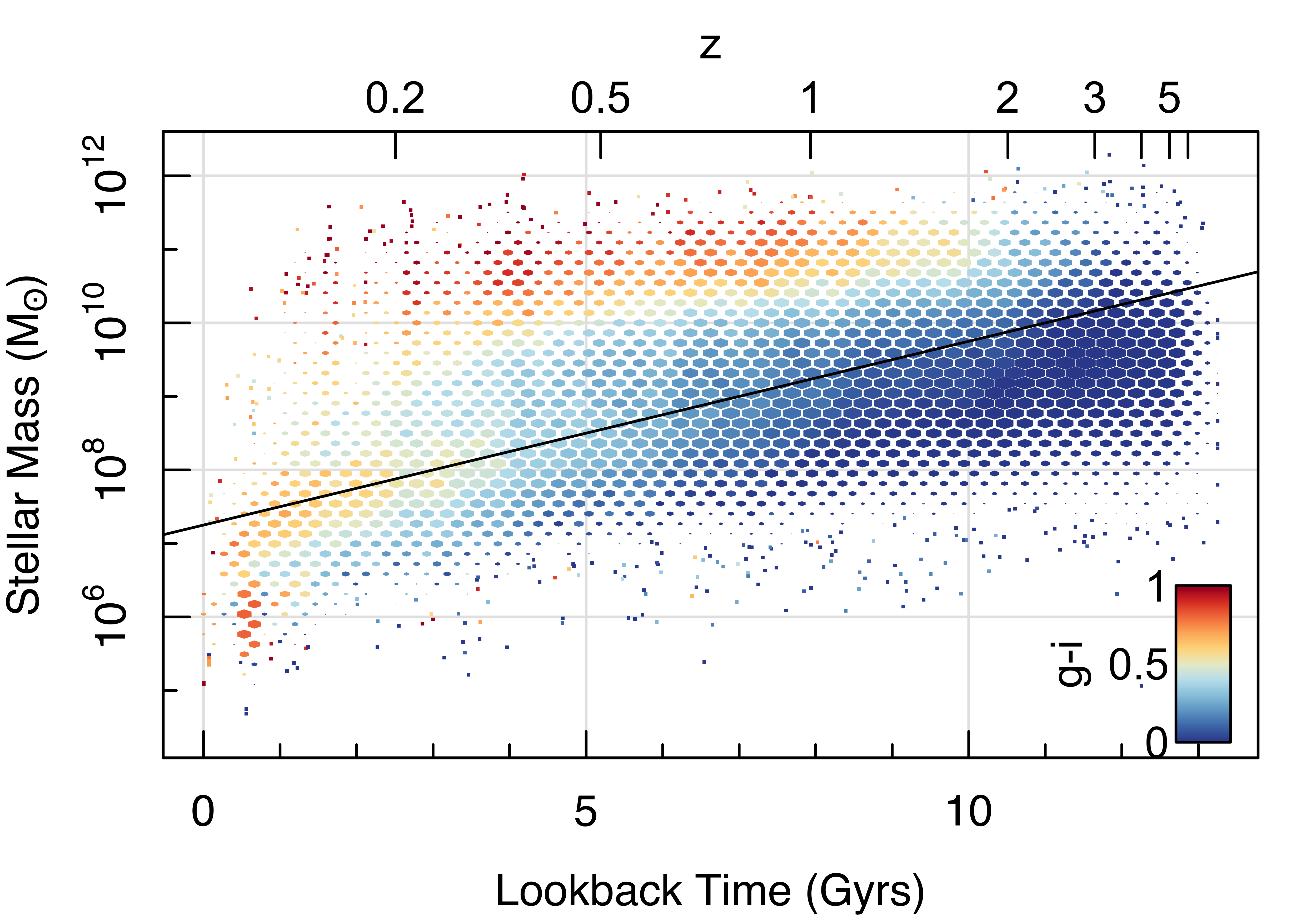
The galaxy stellar mass function (Bell et al. 2003; Baldry et al. 2008; Baldry et al. 2012), is a fundamental tool for studying the evolution of galaxies over cosmic time. Its integral returns the density of baryonic mass currently bound in stars while the shape of the distribution relates to the evolutionary pathways of galaxy growth and assembly. The redshift zero stellar mass function is a key calibration for most galaxy formation models that are carefully tuned to best reproduce the latest measurements (e.g. Crain et al. 2015; Schaye et al. 2015; Lacey et al. 2016; Lagos et al. 2018; Proctor et al. in prep). To compare the galaxy stellar mass distribution measurements obtained from ProSpect to other measurements, we derive the stellar mass function in 15 redshift bins roughly evenly distributed in lookback time. We use all galaxies in these redshift bins regardless of the photometric redshift or the likelihood of the ProSpect fit, but show the impact of making cuts in both in Appendix E.
In this work, as in Driver et al. 2018; Wright et al. 2018, we use only volume-complete samples of the full data set at each redshift interval, thus significantly reducing the possible number of systematic biases that may affect our analysis. Mass completeness limits in each of the redshift bins have been calculated using the unattenuated g-i rest-frame colour as calculated from the ProSpect fits. We show the distribution of stellar mass as a function of lookback time coloured by the median g-i colour in Figure 8. Using this approach, per-bin completeness limits used in this work were estimated by making a linear cut in Figure 8 to limit to mass and redshift bins that were complete (the reddest region in the top left corner). We began with a very conservative cut removing everything below at and compared the differences to the recovered stellar mass functions if we lowered the intercept in 0.25 dex increments. We find no difference in our stellar mass functions when we decrease our intercept to . Where therefore use this relation to make our completeness cut:
| (3) |
where is the lookback time in Gyrs. In each redshift bin we truncate to stellar masses above this cut. This approach is less rigorous than other methods of mass completeness estimate (Marchesini et al. 2009; Muzzin et al. 2013; Tomczak et al. 2014), however is unlikely to bias our analysis over the mass ranges we explore.


Wright et al. 2018 motivate using a two component Schechter 1976 function to model the stellar mass function even out to high redshifts based on the biases induced on the break mass () parameter by a single component Schechter function. They found that fits using a single component Schechter function move to significantly higher values of at early times, causing the regression to behave somewhat poorly. Because of this, we also elect to fit a double Schechter function to our data set in all redshift bins as parameterised as follows:
| (4) |
where , and is the number density as a function of stellar mass.

We use the dftools R package (Obreschkow et al. 2018) to fit Equation 4 in each of the redshift bins. dftools allows for a general modified maximum likelihood method for inferring generative distribution functions from uncertain and biased data. The benefits to using dftools are that it is free of binning and natively accounts for small number statistics, non-detections and simultaneously deals with observational uncertainties (Eddington bias). See Obreschkow et al. 2018 for a complete description of dftools.
When fitting the stellar mass function with dftools we combine the stellar mass uncertainties from ProSpect with the redshift uncertainties for photometric redshift sources to better account for the uncertainty in the stellar mass measurements. We include broad Gaussian priors () on the and parameters based on the predicted values from Wright et al. 2018 and tighter Gaussian priors () on the parameters at and based on the values derived by Wright et al. 2018 and Leja et al. 2020. This allows us to constrain the slopes of the two components especially in our higher redshift bins () where we are not fitting galaxies below . We bootstrap the fits 100 times in each redshift bin to produce more accurate covariances which we show as the shaded region in each panel.
Figure 9 shows the observed number density, binned in stellar mass, with the uncertainties indicated as the per-bin error bars. Each panel shows the best fit double component Schechter as the solid line and the two individual Schechter components as a dotted line in the same colour. We show the extrapolation of the fit at the low mass end as a dashed line of the same colour. All individual fit parameters are presented in Appendix D. We also show comparisons to the stellar mass functions measured by Davidzon et al. 2017; Wright et al. 2018 and Leja et al. 2020 as the dotted grey, dashed black and solid red lines respectively. Davidzon et al. 2017 use the COSMOS2015 catalogue (Laigle et al. 2016) to measure the stellar mass function out to . The measurement from Wright et al. 2018 utilised a combined data set consisting of GAMA, G10-COSMOS (Davies et al. 2015) and 3D-HST (Skelton et al. 2014). They use GAMA to supplement measurements at the low redshift end and use solely 3D-HST for . Note that these stellar mass functions are measured using the masses derived by Driver et al. 2018 which are found to be 0.21 dex lower than the stellar mass estimates derived in this work (Figure 7). Recently Leja et al. 2020 remeasured the stellar mass function using SED fits to the COSMOS2015 (Laigle et al. 2016) and 3D-HST (Skelton et al. 2014) photometry for galaxies between . Leja et al. 2020 fit the stellar mass function over this redshift range using a two-component Schechter function but assuming a ‘continuity model’ which directly fits the evolution of the stellar mass function and ensures a smooth evolution of the parameters. They assume no evolution of the parameters but allow the and parameters to vary in three ‘anchor’ redshifts and assume a quadratic evolution between these redshifts.
We do not correct for large scale structure in any redshift bin which leads to the underestimation of the stellar mass function in the lowest redshift bins () when compared to Wright et al. 2018. This is because Wright et al. 2018 supplement their low redshift measurements with the much larger area of the GAMA survey which is far less prone to impacts from large scale structure. The overestimation of the stellar mass function compared to Wright et al. 2018 between is due to the large clusters known in the COSMOS field (Bellagamba et al. 2011), especially between where there are a large number of known clusters (Finoguenov et al. 2007). Wright et al. 2018 recover lower stellar mass functions across these redshifts due to constraints from GAMA and 3D-HST, whereas we agree closely with the results from Davidzon et al. 2017 as these were also calculated using data purely from the COSMOS field. We also measure lower stellar mass functions at the highest redshifts when compared to both Wright et al. 2018 and Leja et al. 2020 most likely due to the small samples and small mass range over which we can constrain the stellar mass function. In the highest redshift bins () we find minimal contribution from the second Schechter component suggesting that a single Schechter component would be sufficient.
Figure 10 shows a comparison of our derived stellar mass functions to those from simulations. We show comparisons to the stellar mass functions obtained from the semi-analytic model Shark (Lagos et al. 2018), and from the eagle (Schaye et al. 2015) and IllustrisTNG (Pillepich et al. 2018) hydrodynamical simulations. At all redshifts there is reasonable agreement between the theoretical stellar mass functions and ours, with the largest discrepancies at high stellar masses.
4.1 Evolution of the stellar mass function
Figure 11 shows the evolution of the Schechter function parameters, , and . We show comparisons to the double component Schechter fits from Davidzon et al. 2017, Wright et al. 2018 and Leja et al. 2020. We also show the quadratic fit in redshift to the evolution of each parameter from Wright et al. 2018.
As we have not corrected our individual stellar mass functions for the effects of large scale structure, we find that we recover quite different stellar mass functions to previous work in some redshift bins. We isolate redshift bins that are over- or under-dense by fitting a third order smooth spline through the evolution of the density of galaxies with and selecting bins that differ from this spline by more than 50 per cent. These points are shown as open circles in Figure 11 and are excluded from the fits to the evolution of each parameter.
The parameter shows little to no evolution over the redshift range examined and is in very close agreement with the measurements from Wright et al. 2018 and Leja et al. 2020. This is despite the known differences between the stellar masses derived in this work and those used by Wright et al. 2018 (shown in Figure 7) and Leja et al. 2020. We believe this is due to over estimations of the ‘fluxscale’ factor used to correct the aperture derived stellar masses for missing flux as implemented by Wright et al. 2017; Wright et al. 2018.
The value of shows the strongest evolution of any of our fitted parameters with a steep increase over the first Gyr of the Universe, and flattening since. We find no evolution of the parameters as per Wright et al. 2018 and Leja et al. 2020. We find that each of the double component Schechter parameters derived in this work are in agreement with the previous measurements from Wright et al. 2018 and Leja et al. 2020 and differ the most in bins where we find over- or under-densities. We fit the evolution of each of the parameters with a linear fit except for which we fit with a seventh-order polynomial in lookback time as this best recovers the sharp downturn at high lookback time. All SMF fit results and fits to the evolution of each of the parameters are provided in Appendix D.
The stellar mass density shown in Figure 12 is derived using the analytical integration of the regressed Schechter parameters over all masses. By using the regressed values of each of the parameters we assume smooth evolution over cosmic time and are therefore not subject to differences caused by large scale structure. We compare our results to those from Wright et al. 2018, Driver et al. 2018, Davidzon et al. 2017, and the compilation from Madau & Dickinson 2014. We also show comparisons to the inferred stellar mass density evolution from Bellstedt et al. 2020b in orange. This evolution was measured from a sample of low redshift galaxies from the GAMA survey using the ProSpect derived SFHs to trace the entire cosmic SFR and stellar mass density evolution. Our fits show a similar evolution and reasonable agreement with previous work at all redshifts, despite the known 0.2 dex offset between the stellar masses estimates. We expect to be most consistent with the results from Bellstedt et al. 2020b and Leja et al. 2020 as they are both known to recover higher stellar masses than previous work by dex. Over most of cosmic time we find very close agreement with Bellstedt et al. 2020b and differ only at the highest lookback times, where they find a higher stellar mass density than previous measurements. This is unsurprising, as the constraint from SED fitting at this epoch is relatively hard, and hence the Bellstedt et al. 2020b values are most uncertain at this epoch. At high lookback times we agree more closely with the results from Driver et al. 2018 and Madau & Dickinson 2014. We do, however, recover a lower stellar mass density over all cosmic time compared to Leja et al. 2020. This is due to the fact that we recover lower fitted values of at low lookback times, and of at lookback times Gyrs. This results in a slightly lower stellar mass density across all of cosmic time. Despite the higher estimates of stellar mass derived in this work, we find no offset in any of the stellar mass function parameters or resulting stellar mass density from previous measurements.
5 SFR- Relation
The SFR- relation (or the star forming galaxy main sequence, e.g. Brinchmann et al. 2004; Noeske et al. 2007; Salim et al. 2007; Whitaker et al. 2012; Lara-López et al. 2013; Lee et al. 2015; Davies et al. 2016; Davies et al. 2019) is a key diagnostic of both the distribution and evolution of star formation in the Universe. This relation shows the tight correlation between stellar mass and star formation in actively star forming galaxies and is known to evolve in normalisation out to high redshift (e.g. Daddi et al. 2007; Elbaz et al. 2007; Noeske et al. 2007; Lee et al. 2015; Leslie et al. 2020). There is no established consensus in the literature on the proper form of the main sequence; whether it is linear across all redshifts (e.g. Wuyts et al. 2011; Speagle et al. 2014; Pearson et al. 2018), has a flattening or turn-over at stellar masses (e.g. Whitaker et al. 2014; Lee et al. 2015; Schreiber et al. 2015; Leslie et al. 2020) or if any flattening evolves with time. This discrepancy seems to be driven by selection effects. Furthermore, the normalisation of the main sequence relation depends on the SFR tracer and calibrations used (e.g. Speagle et al. 2014; Davies et al. 2016; Davies et al. 2019)
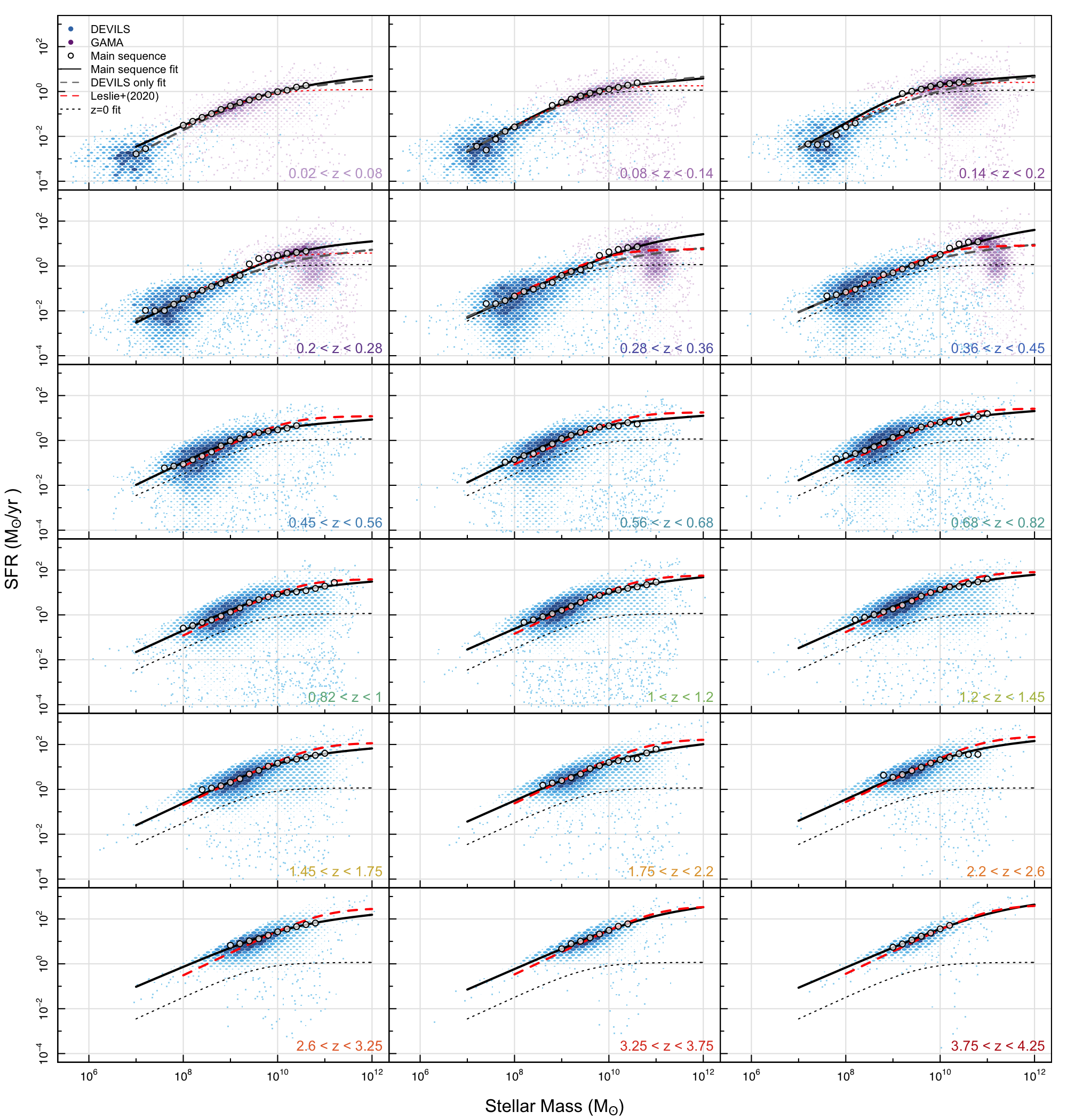
As a final demonstration of our measurements, we present an analysis of the star-formation main sequence relation in the SFR- plane in Figure 13. Whilst we need to be mass complete to measure the galaxy stellar mass function, we only need to be complete in the blue star forming population to measure the main sequence. Because of this we use all objects in our catalogue out to as this is where the median values deteriorate (see Figure 6). To ensure that we have enough high-mass galaxies at low redshift to constrain a potential turn-over, we supplement the DEVILS stellar mass and SFR estimates with ProSpect fits of the subset of publicly available GAMA galaxies as presented in Bellstedt et al. 2020b. The stellar mass and SFR estimates for GAMA were derived in much the same way as the DEVILS estimates derived in this work, with small changes to account for the much smaller redshift range and differing filter set in the photometry catalogue. We supplement the DEVILS measurements with GAMA for redshifts below .
Many methods have been employed in the literature to extract the star forming population including optical colour cuts (Taylor et al. 2015; Davies et al. 2016), specific SFR selections (Guo et al. 2015), or morphological selections (Davies et al. 2019). For this work we elect to split the star forming and passive populations by first making a cut in specific SFR (sSFR) at to remove objects with very low star formation rates that are possible due to the SFH parameterisation. We then fit a mixture model of two Gaussians implemented using the MixTools package (Benaglia et al. 2009) to split the star forming galaxies from the rest of the quenched galaxies. We fit the mixture model in stellar mass bins of width 0.2 dex.
To fit the main sequence we adapt the parameterisation from Lee et al. 2015 which has been shown to hold out to (Tomczak et al. 2016). Equation 2 from Lee et al. 2015 and the adaptation from Leslie et al. 2020 assume a constant SFR at high mass (i.e. a slope of zero), which we do not find evidence for in any redshift bin. We adapt equation 2 from Lee et al. 2015 to add an additional slope to freely model the SFR at high stellar masses:
| (5) |
where and the SFR is measured in . This parameterisation allows us to quantify the interesting characteristics of the relation between stellar mass and SFR: and , the power-law slope at low and high stellar masses respectively, , the turnover mass (in ), and , the maximum value of that the function approaches at high stellar mass.
We provide Normal priors of , and , on the low and high mass slopes respectively. The position of the prior on the low mass slope was selected based on the measurements from Lee et al. 2015 and the assumption of Leslie et al. 2020, whilst the prior on the high mass slope was selected by independently fitting the GAMA data at low redshift with a purely linear relationship. We also implement a broad Normal prior on the turn-over mass, , using the second line of equation 6 from Leslie et al. 2020 to determine the turn over mass at the median redshift of each bin. We use this turn over mass as the mean for the prior and assume a standard deviation of . When fitting our model to the main sequence values, we fit to only mass bins that have more than 300 galaxies. We fit our model to the data using Highlander, assuming a student-t likelihood as it is more robust to outliers due to the heavier tails. We fit Equation 5 to each redshift bin independently. In the low redshift bins where we are supplementing with GAMA measurements, we also fit to only the DEVILS data for comparison. In these cases, the recovered turn-over mass and high-mass slope values are driven by the priors as DEVILS provides no constraint on these parameters on its own. All fit values to the SFR- main sequence are provided in Appendix D.
Figure 13 shows the distribution of all DEVILS and GAMA sources (i.e. star forming and passive) in the SFR- plane as the hexagonal 2D-histogram and the best fit star formation main sequence as obtained in this work in comparison to the recent measurements as derived by Leslie et al. 2020. The measurements from Leslie et al. 2020 are also obtained in the COSMOS field but instead use the COSMOS2015 (Laigle et al. 2016) stellar mass estimates, which are known to be smaller than those measured by ProSpect by approximately 0.2 dex. Leslie et al. 2020 use SFRs derived from 3 GHz radio continuum imaging for their fits. We find very good agreement with the results from Leslie et al. 2020 in all redshift bins but vary most at the high mass end. We do see a discontinuity between the DEVILS and GAMA measurements at intermediate masses between , where the GAMA star formation rates are higher than predicted from DEVILS on its own.
Our fits show clear variation in normalisation across the redshift range with the normalisation increasing to higher redshifts. To compare this evolution to previous results, we take the normalisation at , the high- and low-mass slopes, and the turn-over mass and compare to the results from Damen et al. 2009; Lee et al. 2010; Davies et al. 2016; Leslie et al. 2020 in Figure 14. At low redshift () we show the values derived from fitting only DEVILS as the open circles, and the values including GAMA as the filled circles. We select as our normalization point, as it is well sampled in all redshift bins and is above the incompleteness limits in almost all redshift bins. Note that in some of the low redshift bins is above the turn-over mass, but we find that this does not impact our results. We also overplot measurements from the sSFR evolution from Damen et al. 2009, the low redshift measurements using GAMA from Davies et al. 2016 and other measurements from the COSMOS field from Lee et al. 2015 and Leslie et al. 2020. We correct for the known 0.2 dex offset between the stellar masses used in this work and those used by Lee et al. 2015 and Leslie et al. 2020 by measuring the normalisation from their work at . We also show the fit for the evolution of the main sequence from Speagle et al. 2014, who use a detailed compilation of 25 different samples to evaluate the main sequence out to . Our results are consistent in normalisation with previous work, but we do see some small differences in the low redshift bins. When we include the measurements from GAMA we recover higher normalisations than previous work, but recover lower normalisations when we consider DEVILS on its own.
Whilst the normalisation of the relation is easily compared with other works, the low-mass slope and turn-over mass are harder to compare due to differences in the parameterisation in each work. We compare our measurements of the low-mass slope and turn-over mass to the values from Lee et al. 2015 and Leslie et al. 2020 as their parameterisations only differ from ours in the treatment of the two slope parameters. Leslie et al. 2020 use a fixed low-mass slope with which we find is similar to our measurements at low redshift, but our low-mass slope decreases slightly with increasing redshift despite the prior centered at . We also find that the low-mass slope measurements from Lee et al. 2015 are steeper than our measurements in all redshift bins. Lee et al. 2015 and Leslie et al. 2020 both assume a fixed high-mass slope of zero but we include the variation in our values as a function of lookback time in Figure 14.
The parameterisation used by Leslie et al. 2020 assumes a linear evolution of turn-over mass with lookback time, and whilst we find that our turn-over masses do increase with lookback time, we recover lower turn-over masses across most of the redshift range used by Leslie et al. 2020. Our recovered turn-over mass values in the highest redshift bins () agree very closely with Leslie et al. 2020, but these values are driven by the imposed priors as there are no data at these masses to constrain a turn-over and show no evidence of a turn-over in Figure 13. We expect that this is due to evolution of the main sequence where bending only occurs at low redshift. This is expected to happen as massive galaxies start to undergo quenching at more systematically than at higher redshift (Katsianis et al. 2019) and could be due to the growth of bulge components that contribute to the stellar mass but not to the SFR. This naturally leads to a bending in the main sequence at high masses. The main sequence using DEVILS will be explored further in Thorne et al. (in prep.).
6 Conclusions
We have applied the ProSpect SED-fitting code to 494,000 galaxies between in the D10-COSMOS field of the DEVILS survey. Through the use of a parametric SFH and an evolving metallicity tied to the growth of stellar mass we have recovered stellar and dust mass estimates, SFRs, star formation and metallicity histories and the current gas phase metallicity for each galaxy. In this work we focus on the stellar mass and SFR estimates, but include the dust mass and metallicity estimates in the D10_ProSpectCat DMU. Discussion of metallicities will be deferred to Thorne et al. (in prep) and we stress that the dust masses obtained in this work are heavily dependent on the assumed model and dust temperature which are ill-constrained for a large number of our galaxies due to lack of FIR data.
The results are summarised as follow:
- •
In this work we obtain stellar masses, SFRs and dust masses for 494,000 objects between which will be made publicly available in future DEVILS data releases in the D10_ProSpectCat DMU.
- •
We show comparisons of the stellar masses and SFRs obtained in this work to previous measurements from Laigle et al. 2016 and Driver et al. 2018. Using ProSpect we obtain stellar masses that are 0.2 dex higher than previous measurements due to our physically motivated treatment of metallicity (Section 3).
- •
We use our new stellar mass measurements to measure the stellar mass function for (Section 4). We find good agreement with previous measurements from Davidzon et al. 2017; Wright et al. 2018; Leja et al. 2020 and find no evidence of evolution in the break mass or the two slope parameters (Figure 11). We also find good agreement with previous measurements of the evolution of stellar mass density (Figure 12).
- •
We compare our stellar mass and SFR estimates to previous measurements using the SFR- plane and evolution of the main sequence in Section 5. We find good agreement with previous measurements from Damen et al. 2009; Speagle et al. 2014; Lee et al. 2015; Davies et al. 2016; Leslie et al. 2020. By combining measurements from GAMA with our new DEVILS measurements we see evidence of bending at the high mass end at low redshift () which is not evident using GAMA or DEVILS alone. We also find no evidence of a turn-over in the mass range of our data at high redshift () suggesting that the shape of the main sequence evolves with redshift, where bending only occurs at low redshift. The cause of this will be further explored in Thorne et al. (in prep.)
7 Data Availability
The data products described in this paper are currently available for internal DEVILS team use for proprietary science in the D10_ProSpectCat data management unit (DMU). This DMU will be made public with subsequent DEVILS data releases via data central. The fit values to the galaxy stellar mass function and SFR- main sequence are presented in Appendices D and are available at MNRAS online.
Acknowledgements
We thank the anonymous referee, whose comments improved the paper. JET is supported by the Australian Government Research Training Program (RTP) Scholarship. ASGR and LJMD acknowledge support from the Australian Research Council’s Future Fellowship scheme (FT200100375 and FT200100055 respectively). SB and SPD acknowledge support from the Australian Research Council’s Discovery Project scheme (DP180103740). MS has been supported by the European Union’s Horizon 2020 research and innovation programme under the Maria Skłodowska-Curie (grant agreement No 754510), the National Science Centre of Poland (grant UMO-2016/23/N/ST9/02963) and by the Spanish Ministry of Science and Innovation through Juan de la Cierva-formacion program (reference FJC2018-038792-I). AHW is supported by the European Research Council (Grant No. 770935).
DEVILS is an Australian project based around a spectroscopic campaign using the Anglo-Australian Telescope. The DEVILS input catalogue is generated from data taken as part of the ESO VISTA-VIDEO (Jarvis et al. 2013) and UltraVISTA (McCracken et al. 2012) surveys. DEVILS is part funded via Discovery Programs by the Australian Research Council and the participating institutions. The DEVILS website is https://devilsurvey.org. The DEVILS data is hosted and provided by AAO Data Central (https://datacentral.org.au/).
GAMA is a joint European-Australasian project based around a spectroscopic campaign using the Anglo- Australian Telescope. The GAMA input catalogue is based on data taken from the Sloan Digital Sky Survey and the UKIRT Infrared Deep Sky Survey. Complementary imaging of the GAMA regions is being obtained by a number of in-dependent survey programmes including GALEX MIS, VST KiDS, VISTA VIKING, WISE, Herschel-ATLAS, GMRT and ASKAP providing UV to radio coverage. GAMA is funded by the STFC (UK), the ARC (Australia), the AAO, and the participating institutions. The GAMA website is http://www.gama-survey.org/.
This work was supported by resources provided by the Pawsey Supercomputing Centre with funding from the Australian Government and the Government of Western Australia. We gratefully acknowledge DUG Technology for their support and HPC services.
All of the work presented here was made possible by the free and open R software environment (R Core Team 2020). All figures in this paper were made using the R magicaxis package (Robotham 2016b). This work also makes use of the celestial package (Robotham 2016a) and dftools (Obreschkow 2018).
References
- Adams et al. (2020) Adams N. J., Bowler R. A. A., Jarvis M. J., Häußler B., McLure R. J., Bunker A., Dunlop J. S., Verma A., 2020, MNRAS, 494, 1771
- Aihara et al. (2019) Aihara H., et al., 2019, Publications of the Astronomical Society of Japan, 71, 114
- Alarcon et al. (2021) Alarcon A., et al., 2021, MNRAS, 501, 6103
- Allard & Hauschildt (1995) Allard F., Hauschildt P. H., 1995, ApJ, 445, 433
- Alongi et al. (1993) Alongi M., Bertelli G., Bressan A., Chiosi C., Fagotto F., Greggio L., Nasi E., 1993, A&AS, 97, 851
- Andrews et al. (2017) Andrews S. K., Driver S. P., Davies L. J. M., Kafle P. R., Robotham A. S. G., Wright A. H., 2017, MNRAS, 464, 1569
- Andrews et al. (2018) Andrews S. K., Driver S. P., Davies L. J. M., Lagos C. d. P., Robotham A. S. G., 2018, MNRAS, 474, 898
- Arnouts & Ilbert (2011) Arnouts S., Ilbert O., 2011, Astrophysics Source Code Library, p. ascl:1108.009
- Arnouts et al. (2013) Arnouts S., et al., 2013, A&A, 558, A67
- Baldry et al. (2008) Baldry I. K., Glazebrook K., Driver S. P., 2008, MNRAS, 388, 945
- Baldry et al. (2012) Baldry I. K., et al., 2012, MNRAS, 421, 621
- Baraffe et al. (1998) Baraffe I., Chabrier G., Allard F., Hauschildt P. H., 1998, A&A, 337, 403
- Bell et al. (2003) Bell E. F., McIntosh D. H., Katz N., Weinberg M. D., 2003, ApJS, 149, 289
- Bellagamba et al. (2011) Bellagamba F., Maturi M., Hamana T., Meneghetti M., Miyazaki S., Moscardini L., 2011, MNRAS, 413, 1145
- Bellstedt et al. (2020a) Bellstedt S., et al., 2020a, MNRAS, 496, 3235
- Bellstedt et al. (2020b) Bellstedt S., et al., 2020b, MNRAS, 498, 5581
- Bellstedt et al. (2021) Bellstedt S., et al., 2021, MNRAS, 503, 3309
- Benaglia et al. (2009) Benaglia T., Chauveau D., Hunter D. R., Young D., 2009, J. Stat. Softw., 32, 1
- Bertelli et al. (1994) Bertelli G., Bressan A., Chiosi C., Fagotto F., Nasi E., 1994, A&AS, 106, 275
- Bessell et al. (1989) Bessell M. S., Brett J. M., Scholz M., Wood P. R., 1989, A&AS, 77, 1
- Bessell et al. (1991) Bessell M. S., Brett J. M., Scholz M., Wood P. R., 1991, A&AS, 89, 335
- Boquien et al. (2019) Boquien M., Burgarella D., Roehlly Y., Buat V., Ciesla L., Corre D., Inoue A. K., Salas H., 2019, A&A, 622, A103
- Bressan et al. (1993) Bressan A., Fagotto F., Bertelli G., Chiosi C., 1993, A&AS, 100, 647
- Bressan et al. (2012) Bressan A., Marigo P., Girardi L., Salasnich B., Dal Cero C., Rubele S., Nanni A., 2012, MNRAS, 427, 127
- Brinchmann et al. (2004) Brinchmann J., Charlot S., White S. D. M., Tremonti C., Kauffmann G., Heckman T., Brinkmann J., 2004, MNRAS, 351, 1151
- Bruzual & Charlot (2003) Bruzual G., Charlot S., 2003, MNRAS, 344, 1000
- Calzetti et al. (2000) Calzetti D., Armus L., Bohlin R. C., Kinney A. L., Koornneef J., Storchi-Bergmann T., 2000, ApJ, 533, 682
- Capak et al. (2007) Capak P., et al., 2007, ApJS, 172, 99
- Cardelli et al. (1989) Cardelli J. A., Clayton G. C., Mathis J. S., 1989, ApJ, 345, 245
- Carnall et al. (2018) Carnall A. C., McLure R. J., Dunlop J. S., Davé R., 2018, MNRAS, 480, 4379
- Carnall et al. (2019) Carnall A. C., Leja J., Johnson B. D., McLure R. J., Dunlop J. S., Conroy C., 2019, ApJ, 873, 44
- Casey (2012) Casey C. M., 2012, MNRAS, 425, 3094
- Cassisi et al. (1997a) Cassisi S., degl’Innocenti S., Salaris M., 1997a, MNRAS, 290, 515
- Cassisi et al. (1997b) Cassisi S., Castellani M., Castellani V., 1997b, A&A, 317, 108
- Cassisi et al. (2000) Cassisi S., Castellani V., Ciarcelluti P., Piotto G., Zoccali M., 2000, MNRAS, 315, 679
- Cenarro et al. (2001) Cenarro A. J., Cardiel N., Gorgas J., Peletier R. F., Vazdekis A., Prada F., 2001, MNRAS, 326, 959
- Chabrier (2003) Chabrier G., 2003, PASP, 115, 763
- Charbonnel et al. (1996) Charbonnel C., Meynet G., Maeder A., Schaerer D., 1996, A&AS, 115, 339
- Charbonnel et al. (1999) Charbonnel C., Däppen W., Schaerer D., Bernasconi P. A., Maeder A., Meynet G., Mowlavi N., 1999, A&AS, 135, 405
- Charlot & Fall (2000) Charlot S., Fall S. M., 2000, ApJ, 539, 718
- Chevallard & Charlot (2016) Chevallard J., Charlot S., 2016, MNRAS, 462, 1415
- Choi et al. (2016) Choi J., Dotter A., Conroy C., Cantiello M., Paxton B., Johnson B. D., 2016, ApJ, 823, 102
- Cid Fernandes et al. (2005) Cid Fernandes R., Mateus A., Sodré L., Stasińska G., Gomes J. M., 2005, MNRAS, 358, 363
- Comparat et al. (2015) Comparat J., et al., 2015, A&A, 575, A40
- Conroy (2013) Conroy C., 2013, ARA&A, 51, 393
- Conroy et al. (2009) Conroy C., Gunn J. E., White M., 2009, ApJ, 699, 486
- Cool et al. (2013) Cool R. J., et al., 2013, ApJ, 767, 118
- Crain et al. (2015) Crain R. A., et al., 2015, MNRAS, 450, 1937
- Da Cunha et al. (2008) Da Cunha E., Charlot S., Elbaz D., 2008, MNRAS, 388, 1595
- Daddi et al. (2007) Daddi E., et al., 2007, ApJ, 670, 156
- Dale et al. (2014) Dale D. A., Helou G., Magdis G. E., Armus L., Díaz-Santos T., Shi Y., 2014, ApJ, 784, 83
- Damen et al. (2009) Damen M., Labbé I., Franx M., van Dokkum P. G., Taylor E. N., Gawiser E. J., 2009, ApJ, 690, 937
- Damjanov et al. (2018) Damjanov I., Zahid H. J., Geller M. J., Fabricant D. G., Hwang H. S., 2018, ApJS, 234, 21
- Davidzon et al. (2017) Davidzon I., et al., 2017, A&A, 605, A70
- Davies et al. (2015) Davies L. J. M., et al., 2015, MNRAS, 447, 1014
- Davies et al. (2016) Davies L. J. M., et al., 2016, MNRAS, 461, 458
- Davies et al. (2018) Davies L. J. M., et al., 2018, MNRAS, 480, 768
- Davies et al. (2019) Davies L. J. M., et al., 2019, MNRAS, 483, 1881
- Dotter (2016) Dotter A., 2016, ApJS, 222, 8
- Draine (2003) Draine B. T., 2003, ARA&A, 41, 241
- Draine & Li (2007) Draine B. T., Li A., 2007, ApJ, 657, 810
- Draine et al. (2007) Draine B. T., et al., 2007, ApJ, 663, 866
- Driver et al. (2018) Driver S. P., et al., 2018, MNRAS, 475, 2891
- Eggleton (1971) Eggleton P. P., 1971, MNRAS, 151, 351
- Elbaz et al. (2007) Elbaz D., et al., 2007, A&A, 468, 33
- Eldridge & Stanway (2009) Eldridge J. J., Stanway E. R., 2009, MNRAS, 400, 1019
- Eldridge & Stanway (2019) Eldridge J. J., Stanway E. R., 2019, ArXiv200511883 Astro-Ph, pp 307–328
- Eldridge & Tout (2004) Eldridge J. J., Tout C. A., 2004, MNRAS, 353, 87
- Eldridge et al. (2017) Eldridge J. J., Stanway E. R., Xiao L., McClelland L. A. S., Taylor G., Ng M., Greis S. M. L., Bray J. C., 2017, PASA, 34, e058
- Fagotto et al. (1994a) Fagotto F., Bressan A., Bertelli G., Chiosi C., 1994a, A&AS, 104, 365
- Fagotto et al. (1994b) Fagotto F., Bressan A., Bertelli G., Chiosi C., 1994b, A&AS, 105, 29
- Fanelli et al. (1992) Fanelli M. N., O’Connell R. W., Burstein D., Wu C.-C., 1992, ApJS, 82, 197
- Ferland et al. (1998) Ferland G. J., Korista K. T., Verner D. A., Ferguson J. W., Kingdon J. B., Verner E. M., 1998, PASP, 110, 761
- Ferland et al. (2013) Ferland G. J., et al., 2013, Revista Mexicana de Astronomia y Astrofisica, 49, 137
- Finoguenov et al. (2007) Finoguenov A., et al., 2007, ApJS, 172, 182
- Fluks et al. (1994) Fluks M. A., Plez B., The P. S., de Winter D., Westerlund B. E., Steenman H. C., 1994, A&AS, 105, 311
- Fritz et al. (2006) Fritz J., Franceschini A., Hatziminaoglou E., 2006, MNRAS, 366, 767
- Furlong et al. (2015) Furlong M., et al., 2015, MNRAS, 450, 4486
- Girardi et al. (1996) Girardi L., Bressan A., Chiosi C., Bertelli G., Nasi E., 1996, A&AS, 117, 113
- Girardi et al. (2000) Girardi L., Bressan A., Bertelli G., Chiosi C., 2000, A&AS, 141, 371
- Gräfener et al. (2012) Gräfener G., Owocki S. P., Vink J. S., 2012, A&A, 538, A40
- Gregg et al. (2006) Gregg M. D., et al., 2006, in Koekemoer A. M., Goudfrooij P., Dressel L. L., eds, The 2005 HST Calibration Workshop: Hubble after the Transition to Two-Gyro Mode. p. 209
- Guo et al. (2015) Guo K., Zheng X. Z., Wang T., Fu H., 2015, ApJL, 808, L49
- Han & Han (2012) Han Y., Han Z., 2012, ApJ, 749, 123
- Han & Han (2014) Han Y., Han Z., 2014, ApJS, 215, 2
- Han & Han (2019) Han Y., Han Z., 2019, ApJS, 240, 3
- Hasinger et al. (2018) Hasinger G., et al., 2018, ApJ, 858, 77
- Hsieh et al. (2012) Hsieh B.-C., Wang W.-H., Hsieh C.-C., Lin L., Yan H., Lim J., Ho P. T. P., 2012, ApJS, 203, 23
- Ilbert et al. (2009) Ilbert O., et al., 2009, ApJ, 690, 1236
- Ivanov et al. (2019) Ivanov V. D., Coccato L., Neeser M. J., Selman F., Pizzella A., Dalla Bontà E., Corsini E. M., Morelli L., 2019, A&A, 629, A100
- Jarvis et al. (2013) Jarvis M. J., et al., 2013, MNRAS, 428, 1281
- Johnson et al. (2020) Johnson B. D., Leja J., Conroy C., Speagle J. S., 2020, arXiv e-prints, 2012, arXiv:2012.01426
- Kashino et al. (2019) Kashino D., et al., 2019, ApJS, 241, 10
- Katsianis et al. (2019) Katsianis A., et al., 2019, ApJ, 879, 11
- Kennicutt & Evans (2012) Kennicutt R. C., Evans N. J., 2012, ARA&A, 50, 531
- Kriek et al. (2015) Kriek M., et al., 2015, ApJS, 218, 15
- Kroupa (2001) Kroupa P., 2001, MNRAS, 322, 231
- Kroupa & Boily (2002) Kroupa P., Boily C. M., 2002, MNRAS, 336, 1188
- Kurucz (1992) Kurucz R. L., 1992, in Barbuy B., Renzini A., eds, IAUS Vol. 149, The Stellar Populations of Galaxies. p. 225
- Lacey et al. (2016) Lacey C. G., et al., 2016, MNRAS, 462, 3854
- Lagos et al. (2018) Lagos C. d. P., Tobar R. J., Robotham A. S. G., Obreschkow D., Mitchell P. D., Power C., Elahi P. J., 2018, MNRAS, 481, 3573
- Laigle et al. (2016) Laigle C., et al., 2016, ApJS, 224, 24
- Lançon & Mouhcine (2002) Lançon A., Mouhcine M., 2002, A&A, 393, 167
- Lara-López et al. (2013) Lara-López M. A., et al., 2013, MNRAS, 434, 451
- Le Bertre (1997) Le Bertre T., 1997, A&A, 324, 1059
- Le Borgne et al. (2003) Le Borgne J.-F., et al., 2003, A&A, 402, 433
- Le Fèvre et al. (2013) Le Fèvre O., et al., 2013, A&A, 559, A14
- Le Fèvre et al. (2015) Le Fèvre O., et al., 2015, A&A, 576, A79
- Le Floc’h et al. (2009) Le Floc’h E., et al., 2009, ApJ, 703, 222
- Le Sidaner & Le Bertre (1996) Le Sidaner P., Le Bertre T., 1996, A&A, 314, 896
- Lee et al. (2009) Lee S.-K., Idzi R., Ferguson H. C., Somerville R. S., Wiklind T., Giavalisco M., 2009, ApJS, 184, 100
- Lee et al. (2010) Lee S.-K., Ferguson H. C., Somerville R. S., Wiklind T., Giavalisco M., 2010, ApJ, 725, 1644
- Lee et al. (2015) Lee N., et al., 2015, ApJ, 801, 80
- Lee et al. (2018) Lee K.-G., et al., 2018, ApJS, 237, 31
- Leja et al. (2017) Leja J., Johnson B. D., Conroy C., van Dokkum P. G., Byler N., 2017, ApJ, 837, 170
- Leja et al. (2019) Leja J., Carnall A. C., Johnson B. D., Conroy C., Speagle J. S., 2019, ApJ, 876, 3
- Leja et al. (2020) Leja J., Speagle J. S., Johnson B. D., Conroy C., van Dokkum P., Franx M., 2020, ApJ, 893, 111
- Leslie et al. (2020) Leslie S. K., et al., 2020, ApJ, 899, 58
- Levesque et al. (2010) Levesque E. M., Kewley L. J., Larson K. L., 2010, AJ, 139, 712
- Lilly et al. (2009) Lilly S. J., et al., 2009, ApJS, 184, 218
- Lower et al. (2020) Lower S., Narayanan D., Leja J., Johnson B. D., Conroy C., Davé R., 2020, ApJ, 904, 33
- Lutz et al. (2011) Lutz D., et al., 2011, A&A, 532, A90
- Madau & Dickinson (2014) Madau P., Dickinson M., 2014, ARA&A, 52, 415
- Maiolino & Mannucci (2019) Maiolino R., Mannucci F., 2019, A&AR, 27, 3
- Maraston (2005) Maraston C., 2005, MNRAS, 362, 799
- Maraston et al. (2010) Maraston C., Pforr J., Renzini A., Daddi E., Dickinson M., Cimatti A., Tonini C., 2010, MNRAS, 407, 830
- Marchesini et al. (2009) Marchesini D., van Dokkum P. G., Förster Schreiber N. M., Franx M., Labbé I., Wuyts S., 2009, ApJ, 701, 1765
- Masters et al. (2017) Masters D. C., Stern D. K., Cohen J. G., Capak P. L., Rhodes J. D., Castander F. J., Paltani S., 2017, ApJ, 841, 111
- Masters et al. (2019) Masters D. C., et al., 2019, ApJ, 877, 81
- McCracken et al. (2012) McCracken H. J., et al., 2012, A&A, 544, A156
- Momcheva et al. (2016) Momcheva I. G., et al., 2016, ApJS, 225, 27
- Muzzin et al. (2013) Muzzin A., et al., 2013, ApJ, 777, 18
- Nagamine et al. (2001) Nagamine K., Fukugita M., Cen R., Ostriker J. P., 2001, ApJ, 558, 497
- Nenkova et al. (2008) Nenkova M., Sirocky M. M., Nikutta R., Ivezić Ž., Elitzur M., 2008, ApJ, 685, 160
- Noeske et al. (2007) Noeske K. G., et al., 2007, ApJL, 660, L43
- Noll et al. (2009) Noll S., Burgarella D., Giovannoli E., Buat V., Marcillac D., Muñoz-Mateos J. C., 2009, A & A, 507, 1793
- Nomoto et al. (2013) Nomoto K., Kobayashi C., Tominaga N., 2013, ARA&A, 51, 457
- Obreschkow (2018) Obreschkow D., 2018, Astrophysics Source Code Library, p. ascl:1805.002
- Obreschkow et al. (2018) Obreschkow D., Murray S. G., Robotham A. S. G., Westmeier T., 2018, MNRAS, 474, 5500
- Oesch et al. (2016) Oesch P. A., et al., 2016, ApJ, 819, 129
- Oliver et al. (2012) Oliver S. J., et al., 2012, MNRAS, 424, 1614
- Papovich et al. (2001) Papovich C., Dickinson M., Ferguson H. C., 2001, ApJ, 559, 620
- Paulino-Afonso et al. (2018) Paulino-Afonso A., Sobral D., Darvish B., Ribeiro B., Stroe A., Best P., Afonso J., Matsuda Y., 2018, A&A, 620, A186
- Paxton et al. (2011) Paxton B., Bildsten L., Dotter A., Herwig F., Lesaffre P., Timmes F., 2011, ApJS, 192, 3
- Paxton et al. (2013) Paxton B., et al., 2013, ApJS, 208, 4
- Paxton et al. (2015) Paxton B., et al., 2015, ApJS, 220, 15
- Pearson et al. (2018) Pearson W. J., et al., 2018, A&A, 615, A146
- Pei & Fall (1995) Pei Y. C., Fall S. M., 1995, ApJ, 454, 69
- Pforr et al. (2012) Pforr J., Maraston C., Tonini C., 2012, MNRAS, 422, 3285
- Pickles (1998) Pickles A. J., 1998, PASP, 110, 863
- Pietrinferni et al. (2004) Pietrinferni A., Cassisi S., Salaris M., Castelli F., 2004, ApJ, 612, 168
- Pietrinferni et al. (2013) Pietrinferni A., Cassisi S., Salaris M., Hidalgo S., 2013, A&A, 558, A46
- Pillepich et al. (2018) Pillepich A., et al., 2018, MNRAS, 475, 648
- Planck Collaboration et al. (2016) Planck Collaboration et al., 2016, A&A, 594, A13
- Pols et al. (1995) Pols O. R., Tout C. A., Eggleton P. P., Han Z., 1995, MNRAS, 274, 964
- R Core Team (2020) R Core Team 2020, R: A Language and Environment for Statistical Computing, R Foundation for Statistical Computing
- Rauch (2002) Rauch T., 2002, in Henney W. J., Franco J., Martos M., eds, Revista Mexicana de Astronomia y Astrofisica Conference Series Vol. 12, Revista Mexicana de Astronomia y Astrofisica Conference Series. pp 150–151
- Robotham (2016a) Robotham A. S. G., 2016a, Astrophysics Source Code Library, p. ascl:1602.011
- Robotham (2016b) Robotham A. S. G., 2016b, Astrophysics Source Code Library, p. ascl:1604.004
- Robotham et al. (2018) Robotham A. S. G., Davies L. J. M., Driver S. P., Koushan S., Taranu D. S., Casura S., Liske J., 2018, MNRAS, 476, 3137
- Robotham et al. (2020) Robotham A. S. G., Bellstedt S., Lagos C. d. P., Thorne J. E., Davies L. J., Driver S. P., Bravo M., 2020, MNRAS, 495, 905
- Röck et al. (2015) Röck B., Vazdekis A., Peletier R. F., Knapen J. H., Falcón-Barroso J., 2015, MNRAS, 449, 2853
- Röck et al. (2016) Röck B., Vazdekis A., Ricciardelli E., Peletier R. F., Knapen J. H., Falcón-Barroso J., 2016, A&A, 589, A73
- Salim et al. (2007) Salim S., et al., 2007, ApJS, 173, 267
- Salim et al. (2018) Salim S., Boquien M., Lee J. C., 2018, ApJ, 859, 11
- Salpeter (1955) Salpeter E. E., 1955, ApJ, 121, 161
- Sánchez-Blázquez et al. (2006) Sánchez-Blázquez P., et al., 2006, MNRAS, 371, 703
- Sanders et al. (2007) Sanders D. B., et al., 2007, ApJSS, 172, 86
- Schaller et al. (1992) Schaller G., Schaerer D., Meynet G., Maeder A., 1992, A&AS, 96, 269
- Schaye et al. (2015) Schaye J., et al., 2015, MNRAS, 446, 521
- Schechter (1976) Schechter P., 1976, ApJ, 203, 297
- Schoenberner (1983) Schoenberner D., 1983, ApJ, 272, 708
- Schreiber et al. (2015) Schreiber C., et al., 2015, A&A, 575, A74
- Skelton et al. (2014) Skelton R. E., et al., 2014, ApJS, 214, 24
- Smethurst et al. (2015) Smethurst R. J., et al., 2015, MNRAS, 450, 435
- Smith et al. (2002) Smith L. J., Norris R. P. F., Crowther P. A., 2002, MNRAS, 337, 1309
- Somerville & Primack (1999) Somerville R. S., Primack J. R., 1999, MNRAS, 310, 1087
- Speagle et al. (2014) Speagle J. S., Steinhardt C. L., Capak P. L., Silverman J. D., 2014, ApJS, 214, 15
- Straatman et al. (2018) Straatman C. M. S., et al., 2018, ApJS, 239, 27
- Taylor et al. (2015) Taylor E. N., et al., 2015, MNRAS, 446, 2144
- Tomczak et al. (2014) Tomczak A. R., et al., 2014, ApJ, 783, 85
- Tomczak et al. (2016) Tomczak A. R., et al., 2016, ApJ, 817, 118
- Trayford et al. (2020) Trayford J. W., Lagos C. d. P., Robotham A. S. G., Obreschkow D., 2020, MNRAS, 491, 3937
- Valdes et al. (2004) Valdes F., Gupta R., Rose J. A., Singh H. P., Bell D. J., 2004, ApJS, 152, 251
- Vassiliadis & Wood (1993) Vassiliadis E., Wood P. R., 1993, ApJ, 413, 641
- Vassiliadis & Wood (1994) Vassiliadis E., Wood P. R., 1994, ApJS, 92, 125
- Vazdekis et al. (2016) Vazdekis A., Koleva M., Ricciardelli E., Röck B., Falcón-Barroso J., 2016, MNRAS, 463, 3409
- Walcher et al. (2011) Walcher C. J., Groves B., Budavari T., Dale D., 2011, Ap&SS, 331, 1
- Whitaker et al. (2012) Whitaker K. E., van Dokkum P. G., Brammer G., Franx M., 2012, ApJL, 754, L29
- Whitaker et al. (2014) Whitaker K. E., et al., 2014, ApJ, 795, 104
- Winget et al. (1987) Winget D. E., Hansen C. J., Liebert J., van Horn H. M., Fontaine G., Nather R. E., Kepler S. O., Lamb D. Q., 1987, ApJL, 315, L77
- Worthey (1994) Worthey G., 1994, ApJS, 95, 107
- Wright et al. (2016) Wright A. H., et al., 2016, MNRAS, 460, 765
- Wright et al. (2017) Wright A. H., et al., 2017, MNRAS, 470, 283
- Wright et al. (2018) Wright A. H., Driver S. P., Robotham A. S. G., 2018, MNRAS, 480, 3491
- Wuyts et al. (2011) Wuyts S., et al., 2011, ApJ, 742, 96
- Yang et al. (2020) Yang G., et al., 2020, MNRAS, 491, 740
- Zamojski et al. (2007) Zamojski M. A., et al., 2007, ApJSS, 172, 468
- van Dokkum (2008) van Dokkum P. G., 2008, ApJ, 674, 29
Appendix A Tabular form of Figure 1
| SED Fitting Code | ||||||||
| Template Type | Template | ProSpect | magphys | beagle | prospector | bagpipes | cigale | BayeSED |
| Stellar Templates | BPASS | |||||||
| M05 | ||||||||
| E-MILES | ||||||||
| BC03 | ||||||||
| FSPS | ||||||||
| Dust Attenuation | Cardelli et al. 1989 | |||||||
| Charlot & Fall 2000 | ||||||||
| Salim et al. 2018 | ||||||||
| Calzetti et al. 2000 | ||||||||
| Dust Emission | Dale et al. 2014 | |||||||
| Draine & Li 2007 | ||||||||
| Casey 2012 | ||||||||
| Grey-body | ||||||||
| Initial Mass Function | Chabrier 2003 | |||||||
| Salpeter 1955 | ||||||||
| Kroupa 2001 | ||||||||
| Kroupa & Boily 2002 | ||||||||
| Emission Lines | MAPPINGS-III | |||||||
| CLOUDY | ||||||||
| Star Formation Histories | Parametric | |||||||
| Non-parametric | ||||||||
| Metallicity | Constant but free | |||||||
| Evolving | ||||||||
| AGN Templates | Fritz et al. 2006 | |||||||
| Andrews et al. 2018 | ||||||||
| Casey 2012 | ||||||||
| Dale et al. 2014 | ||||||||
| Nenkova et al. 2008 | ||||||||
| Other | Radio Extension | |||||||
| Spectral Fitting | ||||||||
| X-ray Extension | ||||||||
Appendix B Stellar Template Schematic
Here we show the stellar template counterpart to Figure 1 and Table 3. Interactive versions of both diagrams are available at https://jethorne.github.io/.
| Stellar Template | ||||||
| Template Type | Template | M05 | BPASS | BC03 | FSPS | E-MILES |
| Isochrones | Vassiliadis & Wood 1994 | |||||
| Vassiliadis & Wood 1993 | ||||||
| Winget et al. 1987 | ||||||
| Schoenberner 1983 | ||||||
| Geneva | ||||||
| Cassisi | ||||||
| Cambridge STARS | ||||||
| Padova | ||||||
| Baraffe et al. 1998 | ||||||
| Lançon & Mouhcine 2002 | ||||||
| BaSTI | ||||||
| MIST | ||||||
| PARSEC | ||||||
| Atmospheres / Spectra | Indo-US | |||||
| CAT | ||||||
| NGSL | ||||||
| IRTF | ||||||
| MILES | ||||||
| PoWR | ||||||
| WM Basic | ||||||
| Lançon & Mouhcine 2002 | ||||||
| Pickles | ||||||
| BaSeL | ||||||
| Le Bertre | ||||||
| STELIB | ||||||
| Initial Mass Functions | Salpeter 1955 | |||||
| Kroupa 2001 | ||||||
| Chabrier 2003 | ||||||
| van Dokkum 2008 | ||||||
| Other | ||||||
Appendix C Redshift Sources
Here we present the references for each of the redshift catalogues that were compiled to make the redshift catalogue for this work. Table 5 presents the references for each of the catalogues, the type of redshift, the number and distribution of redshifts used in this work. We also present the flag values from the original catalogues that were selected as good redshifts. In Figure 16 we show the distribution of these redshifts compared with the Y-band magnitude of the object from our photometry catalogue coloured by redshift source.
| Redshift Source | Type | Reference | Nz | Flags | Accuracy | Outlier Rate | ||
|---|---|---|---|---|---|---|---|---|
| DEVILS | Spec | Davies et al. 2018 | 3,394 | 0.509 | [0.0002,1.240] | Prob > 0.9 | ||
| zCOSMOS | Spec | Lilly et al. 2009 | 9,774 | 0.494 | [0.00, 4.447] | * | ||
| hCOSMOS | Spec | Damjanov et al. 2018 | 1,641 | 0.312 | [0.00623,1.26471] | |||
| LEGA-C | Spec | Straatman et al. 2018 | 839 | 0.866 | [0.359, 2.480] | 0 | ||
| VVDS | Spec | Le Fèvre et al. 2013 | 0 | 3 or 4 | ||||
| VUDS | Spec | Le Fèvre et al. 2015 | 126 | 2.510 | [0.00, 4.908] | 1.5,2,3,4,9 | ||
| FMOS | Spec | Kashino et al. 2019 | 285 | 1.557 | [0.895,2.486] | 3,4 | ||
| MOSDEF | Spec | Kriek et al. 2015 | 318 | 2.280 | [0.803, 3.712] | > 4 | ||
| C3R2 | Spec | Masters et al. 2019; Masters et al. 2017 | 2,242 | 0.890 | [0.0625, 4.499] | 3,3.5,4 | ||
| DEIMOS | Spec | Hasinger et al. 2018 | 4,393 | 1.028 | [0.00, 6.604] | 1.5, 2 | ||
| LRIS | Spec | Lee et al. 2018 | 217 | 2.530 | [0.00, 3.029] | |||
| ComparatOII | Spec | Comparat et al. 2015 | 883 | 1.172 | [0.00, 4.816] | |||
| VIS3COS | Spec | Paulino-Afonso et al. 2018 | 348 | 0.839 | [0.0248, 1.261] | |||
| 3D-HST | Grism | Momcheva et al. 2016 | 1,369 | 0.962 | [0.0529, 3.909] | |||
| PRIMUS | Grism | Cool et al. 2013 | 6,149 | 0.698 | [0.0215, 3,485] | |||
| PAU | Photo | Alarcon et al. 2021 | 15,563 | 0.692 | [0.00, 2.990] | 0.009 | 2% | |
| COSMOS2015 | Photo | Laigle et al. 2016 | 411,472 | 1.295 | [0.005, 5.995] | 0.007/0.021† | 0.5%/13.2%† | |
| MIGHTEE | Photo | Adams et al. 2020 | 45,744 | 1.944 | [0.04, 9] | 0.027 | 3.9% |
* Z_CC>2 & Z_CC<6, or Z_CC>12 & Z_CC<16, or Z_CC>22 & Z_CC<26
for comparison to / respectively


Appendix D Fit Results and Regression Values
| Redshift Range | Mpc | Mpc | SMD / Mpc-3) | |||
|---|---|---|---|---|---|---|
| 0.02 < z < 0.08 | 10.4482 0.22 | -2.6039 0.15 | -3.618 0.19 | -0.4864 0.096 | -1.8497 0.045 | 8.5196 0.021 |
| 0.08 < z < 0.14 | 10.7618 0.075 | -2.4418 0.088 | -3.0725 0.067 | -0.521 0.095 | -1.5937 0.023 | 8.4876 0.022 |
| 0.14 < z < 0.20 | 10.8102 0.078 | -2.8321 0.082 | -3.5971 0.072 | -0.4489 0.092 | -1.7176 0.021 | 8.4578 0.023 |
| 0.2 < z < 0.28 | 10.8063 0.045 | -2.5776 0.052 | -3.1587 0.05 | -0.4473 0.087 | -1.5434 0.018 | 8.4262 0.024 |
| 0.28 < z < 0.36 | 10.7985 0.038 | -2.5317 0.049 | -2.9277 0.04 | -0.391 0.088 | -1.4541 0.016 | 8.3971 0.025 |
| 0.36 < z < 0.45 | 10.7994 0.035 | -2.6343 0.045 | -3.0026 0.038 | -0.3617 0.088 | -1.4773 0.016 | 8.3701 0.026 |
| 0.45 < z < 0.56 | 10.7717 0.03 | -2.7099 0.033 | -3.2329 0.045 | -0.3412 0.083 | -1.5399 0.02 | 8.3419 0.027 |
| 0.56 < z < 0.68 | 10.7692 0.025 | -2.644 0.024 | -3.2558 0.046 | -0.2845 0.076 | -1.5621 0.023 | 8.311 0.028 |
| 0.68 < z < 0.82 | 10.7289 0.021 | -2.5994 0.018 | -3.1678 0.042 | -0.1251 0.075 | -1.5336 0.023 | 8.2725 0.028 |
| 0.82 < z < 1.00 | 10.7964 0.017 | -2.49 0.016 | -3.0578 0.052 | -0.2 0.071 | -1.4206 0.031 | 8.2144 0.029 |
| 1.00 < z < 1.20 | 10.8076 0.02 | -2.8084 0.021 | -3.3484 0.056 | -0.2212 0.08 | -1.5264 0.037 | 8.1284 0.029 |
| 1.20 < z < 1.45 | 10.8208 0.02 | -2.8776 0.03 | -3.347 0.078 | -0.36 0.087 | -1.4332 0.054 | 8.0039 0.028 |
| 1.45 < z < 1.75 | 10.8309 0.019 | -3.0228 0.083 | -3.4117 0.2 | -0.6499 0.11 | -1.2988 0.1 | 7.8402 0.027 |
| 1.75 < z < 2.20 | 10.8065 0.017 | -3.1119 0.073 | -3.8187 0.38 | -0.8028 0.1 | -1.3545 0.13 | 7.6388 0.026 |
| 2.20 < z < 2.60 | 10.8055 0.04 | -3.9046 0.35 | -3.4468 0.076 | -0.5408 0.11 | -1.2697 0.072 | 7.494 0.024 |
| 2.60 < z < 3.25 | 10.7558 0.034 | -4.5695 0.31 | -3.5757 0.044 | -0.4979 0.1 | -1.5065 0.058 | 7.3953 0.023 |
| 3.25 < z < 3.75 | 10.5822 0.041 | -4.677 0.37 | -3.6266 0.054 | -0.5004 0.1 | -1.535 0.087 | 7.3452 0.024 |
| 3.75 < z < 4.25 | 10.7851 0.064 | -4.9476 0.36 | -4.2674 0.07 | -0.4985 0.1 | -1.5213 0.091 | 7.3182 0.024 |
| Parameter | ||
|---|---|---|
| 0.0006 0.001 | 10.7792 0.01 | |
| 0.001 | -2.5825 0.022 | |
| -0.0843 0.001 | -2.6863 0.007 | |
| -0.0007 0.001 | -0.3993 0.022 | |
| 0.0013 0.001 | -1.5138 0.008 |
| Redshift Range | ||||
|---|---|---|---|---|
| 0.02 < z < 0.08 | 0.064 0.0019 | 9.5971 0.011 | 0.9703 0.015 | 0.187 0.038 |
| 0.08 < z < 0.14 | 0.139 0.00076 | 9.452 0.0047 | 1.1515 0.0074 | 0.1576 0.016 |
| 0.14 < z < 0.20 | 0.3174 0.032 | 9.4452 0.056 | 1.1838 0.052 | 0.15 0.0017 |
| 0.20 < z < 0.28 | 0.7597 0.02 | 10.1064 0.012 | 1.0728 0.013 | 0.15 0.017 |
| 0.28 < z < 0.36 | 1.1795 0.019 | 10.6332 0.04 | 0.9618 0.016 | 0.1997 0.039 |
| 0.36 < z < 0.45 | 0.8962 0.0087 | 10.2632 0.013 | 0.893 0.0065 | 0.2528 0.053 |
| 0.45 < z < 0.56 | 0.5551 0.0045 | 9.4763 0.021 | 1.0229 0.039 | 0.15 0.015 |
| 0.56 < z < 0.68 | 0.7267 0.0086 | 9.5132 0.02 | 1.0327 0.02 | 0.15 0.0046 |
| 0.68 < z < 0.82 | 0.9698 0.016 | 9.7331 0.023 | 1.0036 0.027 | 0.1519 0.022 |
| 0.82 < z < 1.00 | 1.1263 0.028 | 9.8598 0.045 | 0.972 0.027 | 0.1714 0.02 |
| 1.00 < z < 1.20 | 1.3363 0.0053 | 10.0925 0.019 | 0.9298 0.02 | 0.1902 0.022 |
| 1.20 < z < 1.45 | 1.4696 0.013 | 10.1153 0.021 | 0.9463 0.035 | 0.1784 0.036 |
| 1.45 < z < 1.75 | 1.5302 0.0092 | 10.1547 0.018 | 0.9931 0.024 | 0.1662 0.02 |
| 1.75 < z < 2.20 | 1.6857 0.0096 | 10.3276 0.021 | 0.9374 0.029 | 0.2101 0.047 |
| 2.20 < z < 2.60 | 1.8791 0.007 | 10.4174 0.017 | 0.9589 0.016 | 0.1903 0.034 |
| 2.6 < z < 3.25 | 1.8457 0.007 | 10.1967 0.018 | 0.8964 0.041 | 0.2021 0.042 |
| 3.25 < z < 3.75 | 2.3238 0.0099 | 10.7865 0.013 | 0.9163 0.0098 | 0.2117 0.05 |
| 3.75 < z < 4.25 | 2.4844 0.0043 | 10.9361 0.0078 | 0.9013 0.0045 | 0.2126 0.05 |
| 4.25 < z < 5.00 | 2.6792 0.0057 | 11.1114 0.0035 | 0.9299 0.0029 | 0.2066 0.042 |
| 5.00 < z < 9.00 | 2.7513 0.013 | 10.9998 0.0098 | 0.9861 0.011 | 0.2019 0.067 |
Appendix E Impact of cuts on the derived stellar mass function
To show the impact of removing galaxies with a ‘poor’ fit in either the photometric redshift or ProSpect SED fit we re-calculate the stellar mass function as per Section 4 using the following cuts. Davidzon et al. 2017 applies a cut on the photometric redshift fits which is found to remove 0.17 per cent of the data in our case. To understand the worst-case scenario of poor fits biasing our results we apply a more conservative cut at for both the photometric redshift fit and the ProSpect fit. A cut was selected as this is where the ProSpect fits begin to visually decline in quality. The distribution of values is shown in Figure 18 with the two cuts shown as the red lines. These cuts remove 37,854 galaxies, of which 17,632 are above our completeness cut (Equation 3). This represents a removal of 10 per cent of the objects above the completeness cut. We propagate this selection to our final stellar mass function fits and as seen in Figure 19, it produces an entirely negligible impact on the results (fit parameters changing by much less than the estimated errors).


