Axion electrodynamics in topological materials
Abstract
One of the intriguing properties characteristic to three-dimensional topological materials is the topological magnetoelectric phenomena arising from a topological term called the term.
Such magnetoelectric phenomena are often termed the axion electrodynamics, since the term has exactly the same form as the action describing the coupling between a hypothetical elementary particle, axion, and a photon.
The axion was proposed about forty years ago to solve the so-called strong CP problem in quantum chromodynamics, and is now considered as a candidate for dark matter.
In this tutorial, we overview theoretical and experimental studies on the axion electrodynamics in three-dimensional topological materials.
Starting from the topological magnetoelectric effect in three-dimensional time-reversal invariant topological insulators, we describe the basic properties of static and dynamical axion insulators whose realizations require magnetic orderings. We also discuss the electromagnetic responses of Weyl semimetals with a focus on the chiral anomaly.
We extend the concept of the axion electrodynamics in condensed matter to topological superconductors, whose responses to external fields can be described by a gravitational topological term analogous to the term.
I Introduction
Conventionally, metals and insulators have been distinguished by the existence of band gaps. In 2005, a novel phase of matter that does not belong to either conventional metals or insulators, called the topological insulator, was discovered Kane2005; Kane2005a; Hasan2009; Qi2011; Ando2013. It is notable that topological insulators have bulk band gaps but also have gapless boundary (edge or surface) states. Furthermore, a topological insulator phase and a trivial insulator phase cannot be connected adiabatically to each other. In other words, bulk band-gap closing is required for the transitions between topologically nontrivial and trivial phases. In addition, before the establishment of the concept of topological insulators, different phases of matter had usually been distinguished from each other by the order parameters which indicate spontaneous symmetry breaking. For example, magnetism can be understood as a consequence of spontaneous spin rotational symmetry breaking. However, from the viewpoint of symmetry analysis, time-reversal invariant topological insulators and time-reversal invariant band insulators cannot be distinguished. The ways to distinguish such topologically nontrivial and trivial insulator phases can be divided into two types (which of course give rise to equivalent results). One way is introducing a “topological invariant” such as invariant Kane2005; Moore2007; Fu2007; Fu2007a, which are calculated from the Bloch-state wave function of the system. The other way is the “topological field theory” Qi2008, which describes the responses of topological phases to external fields and is the focus of this tutorial.
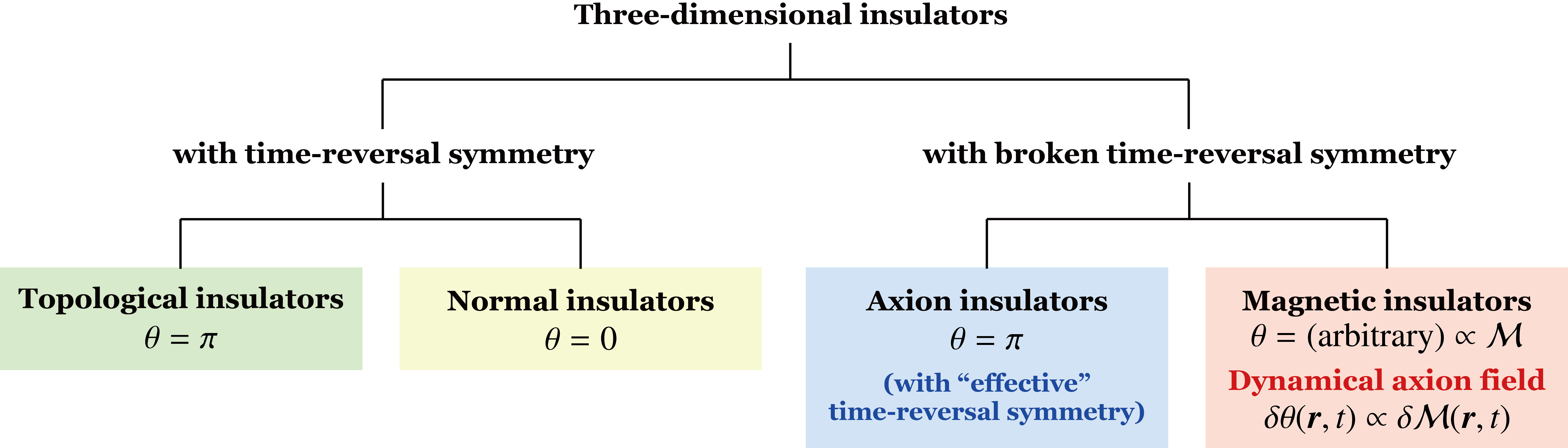
In the topological field theory, the responses of a topological phase to external fields are described by a topological term. In two spatial dimensions, it is well known that the quantum Hall effect of a time-reversal symmetry broken phase can be described by a Chern-Simons action with the quantized coefficient given by the first Chern number Thouless1982; Zhang1992. In three spatial dimensions, time-reversal symmetry plays an important role. The topological magnetoelectric effect described by the so-called term Qi2008 is a hallmark response of three-dimensional (3D) time-reversal invariant topological insulators to external electric and magnetic fields. In the presence of time-reversal symmetry, the coefficient of the magnetoelectric effect takes a quantized value (mod ) for topological insulators, while in trivial insulators. However, in systems with broken time-reversal symmetry e.g., in magnetically ordered phases, the value of can be arbitrary, i.e., can deviate from the quantized value or , which means that the value of can even depend on space and time as . It should be noted that spatial-inversion symmetry breaking can also lead to the deviation of from the quantized value or .
In field theory literature, the phenomena described by the term is termed the axion electrodynamics Wilczek1987, because the term has exactly the same form as the action describing the coupling between a hypothetical elementary particle, axion, and a photon. The axion was proposed about forty years ago to solve the so-called strong CP problem in quantum chromodynamics Peccei1977; Weinberg1978; Wilczek1978. By subsequent studies in particle physics and astrophysics, the axion is now considered as a candidate for dark matter Preskill1983; Abbott1983; Dine1983; book-axions. However, regardless of intensive experimental searches, the axion has not yet been found. Since the coefficient of the term, , is a field describing the axion, observing the magnetoelectric responses in materials whose effective action is described by a term is equivalent to realizing the (dynamical) axion field in condensed matter Li2010. So far, it has been shown theoretically that in a class of magnetic insulators such as magnetically doped topological insulators the value of is proportional to the antiferromagnetic order parameter (i.e., the Néel field), i.e., the antiferromagnetic spin fluctuation is identical to a dynamical axion field Li2010. In Fig. 1, a classification of 3D insulators in terms of the value of is schematically shown.
The effective action of the form of the term appears not only in insulator phases but also in semimetal phases. The key in the case of topological semimetals is the breaking of time-reversal or spatial inversion symmetry, which can lead to nonzero and nonquantized expressions for . For example, in a time-reversal broken Weyl semimetal with two Weyl nodes, its response to external electric and magnetic fields is described by a term with Zyuzin2012; Son2012; Grushin2012; Wang2013; Goswami2013, where is the distance between the two Weyl nodes in momentum space and is the energy difference between the two nodes. In contrast, in the case of topological superconductors, their topological nature is captured only by thermal responses Read2000; Wang2011PRB; Ryu2012, since charge and spin are not conserved. It has been heuristically suggested that the effective action of 3D time-reversal invariant topological superconductors may be described by an action which is analogous to the term but is written in terms of gravitational fields corresponding to a temperature gradient and a mechanical rotation Nomura2012; Shiozaki2013.
In this tutorial, we overview theoretical and experimental studies on the axion electrodynamics in topological materials. In Sec. II we start by deriving the topological magnetoelectric effect described by a term in phenomenological and microscopic ways in 3D time-reversal invariant topological insulators. We also review recent experimental studies toward observations of the quantized magnetoelectric effect. In Sec. III we review the basics and recent experimental realizations of the so-called axion insulators in which the value of is quantized due to a combined symmetry (effective time-reversal symmetry) regardless of the breaking of time-reversal symmetry, focusing on MnBi2Te4 family of materials. In Sec. IV we consider generic expressions for in insulators and extend the derivation of the term in a class of insulators with broken time-reversal and inversion symmetries whose realization requires antiferromagnetic orderings. In Sec. V we describe emergent dynamical phenomena from the realization of the dynamical axion field in topological antiferromagnetic insulators. In Sec. VI and Sec. VII we extend the study of the axion electrodynamics in condensed matter to Weyl semimetals and topological superconductors, respectively, whose effective action can be described by topological terms analogous to the term. In Sec. VIII we summarize this tutorial and outlook future directions of this fascinating research field.
II Quantized magnetoelectric effect in 3D topological insulators
In this section, we describe the basics of the topological magnetoelectric effect, one of the intriguing properties characteristic to 3D topological insulators. We derive phenomenologically and microscopically the term in 3D topological insulators, which is the low-energy effective action describing their responses to external electric and magnetic fields, i.e., the topological magnetoelectric effect. We also review recent theoretical and experimental studies toward observations of the topological magnetoelectric effect.
II.1 Overview
As has been briefly mentioned in the previous section, topological phases can be characterized by their response to external fields. One of the noteworthy characters peculiar to 3D topological insulators is the topological magnetoelectric effect which is described by the so-called term Qi2008. The term is written as
| (1) |
where is the Planck’s constant, is the magnitude of the electron charge, is the speed of light, and and are external electric and magnetic fields, respectively. From the variation of this action with respect to and , we obtain the cross-correlated responses expressed by
| (2) |
with the electric polarization and the magnetization. We see that Eq. (2) clearly exhibits a linear magnetoelectric effect, as schematically illustrated in Fig. 2. Since is odd under time reversal (i.e., under ), time-reversal symmetry requires that the action (1) is invariant under the transformation . Then, it follows that in the presence of time-reversal symmetry takes a quantized value (mod ) for topological insulators, while in trivial insulators. A simple and intuitive proof of this quantization has been given Vazifeh2010. However, in systems with broken time-reversal symmetry e.g., in magnetically ordered phases, the value of can be arbitrary, i.e., can deviate from the quantized value or Essin2009, which means that the value of can even depend on space and time as . A similar argument can be applied to spatial inversion symmetry. Namely, takes a quantized value or (mod ) in the presence of inversion symmetry Hughes2011; Turner2012, and inversion symmetry breaking can also lead to the deviation of from the quantized value, because is also odd under spatial inversion. Table 1 shows the constraints on the value of by time-reversal and spatial-inversion symmetries.

| Time reversal | Inversion | Value of (mod ) |
| ✓ | ✓ | or |
| ✓ | or | |
| ✓ | or | |
| arbitrary |
II.2 Symmetry analysis of the magnetoelectric coupling
The magnetoelectric effect is the generation of bulk electric polarization (magnetization) by an external magnetic (electric) field. The linear magnetoelectric coupling coefficient is generically described by
| (3) |
where indicates spatial direction, and are external electric and magnetic fields, and and are the electric polarization and the magnetization. In general, both time-reversal and spatial-inversion symmetries of the system must be broken, since the occurrence of nonzero () breaks spatial inversion (time-reversal) symmetry. This requirement is consistent with the constraints on the value of by time-reversal and spatial-inversion symmetries (see Table 1). Among several origins of the magnetoelectric effect, we are particularly interested in the orbital (i.e., electronic band) contribution to the linear magnetoelectric coupling of the form:
| (4) |
where is the Kronecker delta. Here, note that is a dimensionless constant. Equation (4) implies the Lagrangian density , since the magnetization and polarization can be derived from the free energy of the system as and . Notably, the susceptibility of the topological magnetoelectric effect in Eq. (4) with reads (in SI units)
| (5) |
which is rather large compared to those of prototypical magnetoelectric materials, e.g., the total linear magnetoelectric susceptibility of the well-known antiferromagnetic Cr2O3 at low temperatures Wiegelmann1994; Coh2011.
It should be noted here that we need to take into account the presence of boundaries (i.e., surfaces) of a 3D topological insulator, when we consider the realization of the quantized magnetoelectric effect in a 3D topological insulator. This is because, as is mentioned just above, finite and require the breaking of both time-reversal and spatial inversion symmetries of the whole system, whereas the bulk of the topological insulator has to respect both time-reversal and inversion symmetries. As we will see in the following, the occurrence of the quantized magnetoelectric effect is closely related to the (half-quantized) anomalous Hall effect on the surface, which requires a somewhat special setup that breaks both time-reversal and inversion symmetries as shown in Fig. 2. In this setup, time-reversal symmetry is broken due to the surface magnetization. Inversion symmetry is also broken because the magnetization directions on a side surface and the other side surface are opposite to each other (spatial inversion does not change the direction of spin).
II.3 Surface half-quantized anomalous Hall effect
Before deriving the quantized magnetoelectric effect in 3D topological insulators, we briefly consider the anomalous Hall effect on the surfaces in which the Hall conductivity takes a half-quantized value . Let us start with the effective Hamiltonian for the surface states of 3D topological insulators such as Bi2Se3, which is described by 2D two-component massless Dirac fermions Zhang2009:
| (6) |
where is the Fermi velocity of the surface state (i.e., the slope of the Dirac cone), and are the Pauli matrices for the spin degree of freedom. The energy eigenvalues of the Hamiltonian (6) are readily obtained as from a simple algebra . The Fermi velocity of the surface states in Bi2Se3 is experimentally observed as m/s Xia2009.
Due to the spin-momentum locking, the surface states are robust against disorder, as long as time-reversal symmetry is preserved. Namely, the backscattering of surface electrons from to are absent Roushan2009. Theoretically, it has been shown that 2D two-component massless Dirac fermions cannot be localized in the presence of nonmagnetic disorder Bardarson2007; Nomura2007. However, surface states are not robust against magnetic disorder which breaks time-reversal symmetry. This is because the surface Dirac fermions described by Eq. (6) can be massive by adding a term proportional to , i.e., , which opens a gap of in the energy spectrum. More precisely, such a mass term can be generated by considering the exchange interaction between the surface electrons and magnetic impurities Liu2009; Abanin2011; Nomura2011 such that , where is the impurity spin at position . Then, the homogeneous part of the impurity spins gives rise to the position-independent Hamiltonian
| (7) |
where is the density of magnetic impurities and is the averaged spin of magnetic impurities. Adding Eq. (7) to the Hamiltonian (6) leads to a gapped spectrum
| (8) |
We see that and do not open the gap but only shift the position of the Dirac cone in momentum space.

Let us consider a general Hamiltonian given by . In the case of massive Dirac fermions, is given by . The Hall conductivity of the system with the Fermi level being in the gap can be calculated by Volovik-book
| (9) |
where is a unit vector. The integral is equivalent to the area where the unit vector moves on the unit sphere, which namely gives the winding number of . At , the unit vector points the north or south pole, that is, . At large with , almost points the horizontal directions. Hence, varying , covers the half of the unit sphere, which gives .
Equation (9) indicates the anomalous Hall effect occurs on the surfaces of 3D topological insulators, when magnetic impurities are doped or a magnetic film is put on the surfaces Yu2010; Nomura2011. The direction of the Hall current depends on the sign of , i.e., the direction of the magnetization of magnetic impurities or proximitized magnetization. Actually, the surface quantum anomalous Hall effect has been observed experimentally Chang2013; Checkelsky2014. The observed surface quantum anomalous Hall effect in a thin film of Cr-doped (Bi,Sb)2Te3 is shown in Fig. 3. Note that in those systems the magnetization directions of top and bottom surfaces are the same, and thus the observed Hall conductivity is . It can be seen from Fig. 3(b) that the Hall conductivity takes the quantized value when the chemical potential lies in the surface bandgap.
II.4 Phenomenological derivation of the term
We have seen in the previous section that the surface states of 3D topological insulators can be gapped (i.e., the surface Dirac fermions can be massive) via the exchange interaction with magnetic impurities or proximitized magnetization which breaks time-reversal symmetry, giving rise to the surface half-quantized anomalous Hall effect. We show phenomenologically in the following that, as a consequence of the surface half-quantized anomalous Hall effect, the topological magnetoelectric effect [Eq. (2)] emerges in 3D topological insulators.
Let us consider a case where the side surface of a cylindrical 3D topological insulator is ferromagnetically ordered due to magnetic doping or proximity effect Qi2008, as shown in Fig. 2. The resulting surface Dirac fermions are massive. When an external electric field is applied parallel to the cylinder, the surface anomalous Hall current is induced as
| (10) |
where is a unit vector normal to the side surface. From the Ampère’s law, the magnetization with ( is the speed of light) is obtained as [see Fig. 2(a)]
| (11) |
Similarly, when an external magnetic field is applied parallel to the cylinder, the circulating electric field normal to the magnetic field is induced as . Then the induced electric field generates the surface anomalous Hall current parallel to the magnetic field as
| (12) |
On the other hand, a polarization current is equivalent to the time derivative of the electric polarization. Finally the induced electric polarization is given by [see Fig. 2(b)]
| (13) |
Equations (11) and (13) clearly show the magnetoelectric effect. Here, recall that the magnetization and polarization can be derived from the free energy of the system as and . To satisfy the relations (11) and (13), the free energy must have the following form Qi2008:
| (14) |
where we have omitted for simplicity, and . The integrand can be regarded as the Hamiltonian density. The equivalent action is written as
| (15) |
where , with being the electromagnetic four-potential, and is the Levi-Civita symbol with the convention . Here, the electric field and magnetic field are given respectively by and . Note that () is the fine-structure constant. Equation (15) is indeed the term [Eq. (1)]. Under time reversal (), electric and magnetic fields are transformed as and , respectively. Similarly, under spatial inversion (), electric and magnetic fields are transformed as and , respectively. Hence, the term is odd under time reversal or spatial inversion. On the other hand, 3D topological insulators have time-reversal symmetry, which indicates that remains unchanged under time reversal. In other words, the value of must be invariant under the transformation . It follows that (mod ) in time-reversal invariant topological insulators and in normal (topologically trivial) insulators.
Note that is a surface term when the value of is constant, i.e., independent of spatial coordinate and time, since we can rewrite the integrand of in a total derivative form,
| (16) |
which indicates that the topological magnetoelectric effect in the bulk is a consequence of the surface response to the electric and magnetic fields. However, as we shall see later, the presence of the term that is dependent of spatial coordinate and/or time results in an electric current generation in the bulk.
Here, let us consider the inverse process of the derivation of the term (15). Namely, we derive the surface anomalous Hall current from Eq. (15). We have seen in Eq. (16) that the integrand of the term is a total derivative when the value of is constant. For definiteness, let us see what happens at a given surface in the direction. Using Eq. (16) and integrating out with respect to , the surface term can be obtained from Eq. (15) as
| (17) |
where . Recall that, in general, an electric current density in the direction can be obtained from the variation of an action with respect to the electromagnetic vector potential : . Without loss of generality we may consider the current in the direction,
| (18) |
where is the electric field in the direction. Since in topological insulators, Eq. (18) clearly shows the surface half-quantized anomalous Hall effect.
More precisely, we should consider an electric current derived directly from the term. Namely, we should consider the spatial dependence of such that in vacuum and inside the topological insulator. Notice that the term can be rewritten as
| (19) |
Then the electric current density is obtained as
| (20) |
The magnetic-field induced term is the so-called chiral magnetic effect Fukushima2008, which will be mentioned later. For concreteness, we require that the region () be the topological insulator (vacuum). The dependence of can be written in terms of the Heaviside step function as , since () inside (outside) the topological insulator. Then, we obtain , which gives rise to the half-quantized Hall conductivity at the topological insulator surface .
II.5 Microscopic derivation of the term
So far we have derived the topological magnetoelectric effect [Eq. (2)] from a surface property of 3D topological insulators. In this section, we derive the term microscopically from a low-energy effective model of 3D topological insulators. There are several ways to derive the term microscopically. One way is to use the so-called Fujikawa’s method Fujikawa1979; Fujikawa1980. Another way is the dimensional reduction from (4+1)-dimensions to (3+1)-dimensions Qi2008, which will be briefly mentioned in Sec. IV.1. Here, we show the derivation of the term based on Fujikawa’s method.
II.5.1 Effective Hamiltonian for 3D topological insulators
Let us start from the low-energy continuum model for prototypical 3D topological insulators such as Bi2Se3. The bulk electronic structure of Bi2Se3 near the Fermi level is described by two -orbitals and with denoting parity. Defining the basis and retaining the wave vector up to quadratic order, the low-energy effective Hamiltonian around the point is given by Zhang2009; Liu2010
| (21) |
where and . The coefficients for Bi2Se3 estimated by a first-principles calculation read eV, eVÅ, eVÅ, eVÅ2, and eVÅ2 Zhang2009; Liu2010. Here, note that we have introduced a basis in Eq. (21) that is slightly different from that Refs. Zhang2009; Liu2010. The matrices are given by the so-called Dirac representation,
| (22) | ||||
where the Clifford algebra is satisfied. The above Hamiltonian is nothing but an anisotropic 3D Dirac Hamiltonian with a momentum-dependent mass.
Before proceeding to the derivation of the term, it is informative to consider the lattice version of Eq. (21). Here, recall that the invariant Kane2005; Fu2007; Fu2007a; Moore2007, which identifies whether a phase is topologically nontrivial or trivial, is calculated in lattice models. This means that we cannot directly show that the phase described by the effective Hamiltonian (21) represents a 3D topological insulator. From this viewpoint, we need to construct a lattice Hamiltonian from the continuum Hamiltonian (21). The simplest 3D lattice is the cubic lattice. We replace and terms by and . Although this replacement is valid only when , as is shown below, it turns out that this replacement describes the topological insulator phase. We also simplify the coefficients to obtain the isotropic lattice Hamiltonian
| (23) |
where we have defined and . As is mentioned below, the Hamiltonian (23) is also called the Wilson-Dirac Hamiltonian Wilson1977; Creutz1994; Sekine2013, which was originally introduced in lattice quantum chromodynamics.
In cubic lattices, the eight time-reversal invariant momenta , which are invariant under , are given by , , , , , , , and where is the lattice constant. We can calculate the invariant of the system as Fu2007; Fu2007a
| (24) |
Indeed, the topological insulator phase with satisfies the above realistic value for Bi2Se3; , where we have assumed the value of the lattice constant as Å.
It should be noted here that the lattice Dirac Hamiltonian (23) is exactly the same as the Hamiltonian of the Wilson fermions, which was originally introduced in lattice gauge theory to avoid the fermion doubling problem Wilson1977. Namely, we can see that Eq. (23) around the point represents the usual (continuum) massive Dirac fermions with the mass , while Eq. (23) around other momentum points, e.g., , represent massive Dirac fermions with the mass .
II.5.2 Fujikawa’s method
Now, let us return to the continuum Hamiltonian (21) to obtain the term. As we have seen in Eq. (24), the lattice Hamiltonian (23) describes a topological insulator when . Without loss of generality, we can set and . Then, the Hamiltonian (21) with and , which describes a topological insulator, around the point can be simplified by ignoring the terms second-order in as
| (25) |
where . Except for the negative mass , this is the usual Dirac Hamiltonian. In the presence of an external electromagnetic vector potential , minimal coupling results in , with being the magnitude of the electron charge. In the presence of an external electromagnetic scalar potential , the energy density is modified as . Using these facts, the action of the system in the presence of an external electromagnetic four-potential is written in the usual relativistic form Peskin-Schroeder-Book
| (26) |
where is a fermionic field representing the basis of the Hamiltonian (21) and . Here, the gamma matrices are given by the so-called Dirac representation as
| (27) |
which satisfy the relation with being the metric tensor. It is convenient to study the system in the imaginary time notation, i.e., in Euclidean spacetime. Namely, we rewrite , , and as , , and (). The Euclidean action of the system is then written as
| (28) |
where we have used the fact that . Note that and are unchanged ( and ), so that the anticommutation relation is satisfied. Note also that, in Euclidean spacetime, we do not distinguish between superscripts and subscripts.
Now, we are in a position to apply Fujikawa’s method Fujikawa1979; Fujikawa1980 to the action (28). First let us consider an infinitesimal chiral transformation defined by
| (29) |
where . Then the partition function is transformed as
| (30) |
The term comes from the Jacobian defined by . The action (28) is transformed as
| (31) |
The Jacobian is written as Fujikawa1979; Fujikawa1980
| (32) |
Here and we have written and explicitly. We repeat this procedure infinite times, i.e., integrate with respect to the variable from to . Due to the invariance of the partition function, finally we arrive at the following expression of :
| (33) |
where we have dropped the irrelevant surface term. The first term is the action of a topologically trivial insulator, since the mass is positive. The second term is the term in imaginary time, and we obtain Eq. (15) by substituting .
II.6 Toward observations of the topological magnetoelectric effect
II.6.1 Utilizing topological insulator thin films

As we have seen in Sec. II.4, the experimental realization of the topological magnetoelectric effect in topological insulators requires that all the surface Dirac states are gapped by magnetic proximity effect or magnetic doping, resulting in the zero anomalous Hall conductivity of the system. However, such an experimental setup is rather difficult to to be realized. As an alternate route to realize the topological magnetoelectric effect, it has been proposed theoretically that the quantum Hall state, which attributes to the difference between the Landau levels of the top and bottom surface Dirac states, can be utilized Morimoto2015; Wang2015. The quantum Hall state has been experimentally observed in topological insulator (Bi1-xSbx)2Te3 films Yoshimi2015, as shown in Fig. 4(a). The two-component Dirac fermions in a magnetic field are known to show the quantum Hall effect with the Hall conductivity
| (34) |
where is an integer. Note that, as we have seen in Eq. (9), the contribution arises as a Berry phase effect. The total Hall conductivity contributed from the top and bottom surfaces of a topological insulator film in a magnetic field is then written as
| (35) |
The quantum Hall state is realized when the Landau levels of the top and bottom surface states are and (and vice versa), where is an integer Morimoto2015. This state corresponds to and in Eq. (35), which can be achieved in the presence of an energy difference between the two surface states, as shown in Fig. 4(b). Here, recall that the electron density is given by , with the magnetic field strength and the elementary charge. Using this fact, the charge densities () at the top and bottom surfaces are obtained as and , respectively. We consider the case of , which is experimentally relevant Yoshimi2015. The induced electric polarization in a topological insulator film of thickness reads
| (36) |
which is indeed the topological magnetoelectric effect with the quantized coefficient . Note that the case of , which gives rise to , still describes the topological magnetoelectric effect, since modulo .


Another route to realize the topological magnetoelectric effect is a magnetic heterostructure in which the magnetization directions of the top and bottom magnetic insulators are antiparallel Morimoto2015; Wang2015. Several experiments have succeeded in fabricating magnetic heterostructures that exhibits a zero Hall plateau Mogi2017; Mogi2017a; Xiao2018. In Ref. Mogi2017, a magnetic heterostructure consisting of a magnetically doped topological insulator Cr-doped (Bi,Sb)2Te3 and a topological insulator (Bi,Sb)2Te3 was grown by molecular beam epitaxy. A zero Hall conductivity plateau was observed in this study as shown in Fig. 5, implying an axion insulator state. In Ref. Xiao2018, a magnetic heterostructure of a topological insulator (Bi,Sb)2Te3 sandwiched by two kinds of magnetically doped topological insulators V-doped (Bi,Sb)2Te3 and Cr-doped (Bi,Sb)2Te3 was grown by molecular beam epitaxy. Importantly, as shown in Fig. 6, the antiparallel magnetization alignment of the top and bottom magnetic layers was directly observed by magnetic force microscopy when the system exhibited a zero Hall resistivity plateau. Note, however, that the above experiments did not make a direct observation of the magnetoelectric effect, i.e., the electric polarization induced by a magnetic field or the magnetization induced by an electric field.
II.6.2 Faraday and Kerr rotations

As has been known in particle physics Sikivie1983; Wilczek1987 before the discovery of 3D topological insulators, the term modifies the Maxwell’s equations. Since the Maxwell’s equations describe electromagnetic wave propagation in materials, the presence of the term leads to unusual optical properties such as the quantized Faraday and Kerr rotations in topological insulators Qi2008; Tse2010; Maciejko2010 which can be viewed as as a consequence of the topological magnetoelectric effect. To see this, let us start from the total action of an electromagnetic field in the presence of a term is given by
| (37) |
where is the fine-structure constant and is the electromagnetic field tensor. The electric and magnetic fields are respectively given by and . Note that and . Here, recall that the classical equation of motion for the field is obtained from the Euler-Lagrange equation:
| (38) |
where is the Lagrangian density of the system. From Eqs. (37) and (38), one finds that the Maxwell’s equations are modified in the presence of a term Sikivie1983; Wilczek1987; Qi2008
| (39) |
The terms in Eq. (39) play roles when there is a boundary, e.g., gives rise to the surface Hall current as we have seen in Eq. (20).

The modified Maxwell’s equations (39) can be solved under the boundary conditions (see Fig. 7). It is found that the Faraday and Kerr rotation angles are independent of the material (i.e., topological insulator thin film) parameters such as the dielectric constant and thickness Tse2010; Maciejko2010. Especially, in the quantized limit the Faraday and Kerr rotation angles are given respectively by Tse2010; Maciejko2010
| (40) |
These quantized angles have been experimentally observed in the anomalous Hall state Okada2016 and the quantum Hall state [Fig. 8(a)] Wu2016; Dziom2017. Also, as predicted in Ref. Maciejko2010, a universal relationship in units of the fine-structure constant between the Faraday and Kerr rotation angles has been observed [Fig. 8(b)] Okada2016; Wu2016.
III Axion insulators
In Sec. II we have seen that the topological magnetoelectric effect with the quantized coefficient (mod ) occurs in 3D time-reversal invariant topological insulators. In general, the value of is no longer quantized and becomes arbitrary in systems with broken time-reversal symmetry. However, in a class of 3D antiferromagnetic insulators, an “effective” time-reversal symmetry represented by a combination of time-reversal and a lattice translation is present, leading to the topological magnetoelectric effect with the quantized coefficient (mod ). In this section, we review theoretical and experimental studies on such antiferromagnetic topological insulators which are also called the axion insulators. Starting from the basics of the antiferromagnetic topological insulators, we focus on the MnBi2Te4 family of materials which are layered van der Waals compounds and have recently been experimentally realized.
III.1 Quantized magnetoelectric effect in antiferromagnetic topological insulators
Following Ref. Mong2010, we consider a class of insulators in which time-reversal symmetry is broken but the combined symmetry of time reversal and a lattice translation is preserved. We note here that the presence or absence of inversion symmetry does not affect their topological classification, although the presence of inversion symmetry greatly simplifies the evaluation of their topological invariants as in the case of time-reversal invariant topological insulators Fu2007. Let us start from some general arguments on symmetry operations. The time-reversal operator for spin-1/2 systems is generically given by with , where are Pauli matrices and is complex conjugation operator. In the presence of time-reversal symmetry, the Bloch Hamiltonian of a system satisfies
| (41) |
Recall that momentum is the generator of lattice translation. An operator that denotes a translation by a vector is given by . Then, the translation operator that moves a lattice by half a unit cell in the direction is written as
| (42) |
where is a primitive translation vector and is an identity operator that acts on the half of the unit cell Mong2010. One can see that gives a translation by because .

Now, we consider the combination of and defined by . It follows that , which means that the operator is antiunitary like . Here, we have used the fact that and are commute. Note, however, that only on the Brillouin-zone plane satisfying , while . When a system is invariant under the operation , the Bloch Hamiltonian satisfies
| (43) |
which has the same property as time-reversal symmetry in Eq. (41). Therefore, the topological classification can also be applied in systems with the symmetry Mong2010; Fang2013. Figure 9 shows a schematic illustration of an antiferromagnetic topological insulator protected by the symmetry. In this simple model, the unit cell consists of nonmagnetic equivalent and atomic layers, and antiferromagnetically ordered and atomic layers. The half-uni-cell translation moves the layer to the layer, and time reversal changes a spin-up state into a spin-down state. Therefore, the system is obviously invariant under the transformation.
Next, let us consider the resulting surface states. Since on the Brillouin-zone plane satisfying , the 2D subsystem on the plane is regarded as a quantum spin Hall system with time-reversal symmetry. This means that the or dependence of the surface spectra must be gapless, because the line of the surface states is the boundary of 2D subsystem (the plane) in the bulk Brillouin zone. In other words, at the surfaces that are parallel to , which preserve the symmetry, there exist an odd number of gapless surface states (as in the case of a strong time-reversal invariant topological insulator). On the other hand, at the surfaces that are perpendicular to , which break the symmetry, such a topological protection of the surface states no longer exists, and the surface states can have gapped spectra.
As we have seen above, the presence of symmetry results in a realization of a new 3D topological insulator. This implies that such topological insulators exhibit a quantized magnetoelectric effect described by a term, as in the case of time-reversal invariant 3D topological insulators. To see this, recall that the magnetoelectric effect resulting from a term is expressed as , and , where and are the electric polarization and the magnetization, respectively. Under time reversal , the coefficient changes sign , because and while and . On the other hand, the lattice translation does not affect Mong2010. Combining these, the operation implies the transformation such that with being an integer. Then, it follows that or modulo .
III.2 MnBi2Te4
III.2.1 Electronic structure of MnBi2Te4 bulk crystals

With the knowledge of antiferromagnetic topological insulators with the symmetry, here we review recent experimental realizations of the antiferromagnetic topological insulator state in MnBi2Te4 Otrokov2019; Zhang2019; Li2019; Lee2019; Chen2019a; Vidal2019; Hao2019; Li2019PRX; Chen2019; Gong2019; Yan2019. The crystal structure of MnBi2Te4 is shown in Fig. 10. The septuple layer consisting of Te-Bi-Te-Mn-Te-Bi-Te is stacked along the [0001] direction by van der Waals forces. A theoretical calculation of the exchange coupling constants between Mn atoms shows that the intralayer coupling in each Mn layer is ferromagnetic, while the interlayer coupling between neighboring Mn layers is antiferromagnetic Otrokov2019. The magnetic ground state is thus considered to be antiferromagnetic with the Néel vector pointing the out-of-plane direction (i.e., the direction), which is called A-type AFM-. The Néel temperature is reported to be about Otrokov2019; Lee2019; Chen2019; Yan2019. The unit cell of the antiferromagnetic insulator state consists of two septuple layers (Fig. 10), where is the half-cell translation vector along the axis which connects nearest spin-up and spin-down Mn atomic layers. It can be easily seen that this interlayer antiferromagnetism between the Mn atonic layers preserves the symmetry, indicating that the system is a topological antiferromagnetic insulator which we have discussed in the previous section. Interestingly, the bulk bandgap is estimated to be about 0.2 eV Otrokov2019; Zhang2019, which is comparable to that of the time-reversal invariant topological insulator Bi2Se3.


The A-type AFM- state is invariant under spatial inversion with the inversion center located at the Mn atomic layer in each septuple layers. Importantly, symmetry, the combination of spatial inversion with the inversion center located between two septuple layers and time reversal , is also preserved. The presence of symmetry leads to doubly degenerate bands even in the absence of time-reversal symmetry Tang2016; Li2019; Li2019PRB. Here, following Ref. Zhang2019; Wang2020, we derive the low-energy effective Hamiltonian of the A-type AFM- state. symmetry requires that
| (44) |
since momentum changes sign under both and . As in the case of Bi2Se3 [Eq. (21)], the low-energy effective Hamiltonian of the nonmagnetic state of MnBi2Te4 around the point is written in the basis of , where the states and come from the orbitals of Bi and Te, respectively Zhang2019. In this basis, and , where and act on the orbital and spin spaces, respectively, and is complex conjugation operator. symmetry constrains the possible form of the Bloch Hamiltonian . It follows that the following five matrices and the identity matrix are allowed by symmetry:
| (45) |
due to the property . Note that these five matrices anticommute with each other, leading to doubly degenerate energy eigenvalues. Using these five matrices, the low-energy effective Hamiltonian around the point is written as Zhang2019; Wang2020
| (46) |
where . The mass is induced by the antiferromagnetic order. One can see that the Hamiltonian (46) is invariant under both and when . Indeed, the surface states of the lattice model constructed from Eq. (46) in a slab geometry in the direction exhibit the half-quantized anomalous Hall conductivity , implying the axion insulator state Wang2020.
The surface states of antiferromagnetic MnBi2Te4 are somewhat complicated. Theoretical studies have predicted that the (0001) surface state (i.e., at the surface perpendicular to the axis) which breaks the symmetry of the A-type AFM- state is gapped Otrokov2019; Zhang2019, as indicated by the property of antiferromagnetic topological insulators (see Sec. III.1). The first experimental study reported that the (0001) surface state is gapped Otrokov2019. However, subsequent studies reported that it is gapless Hao2019; Li2019PRX; Chen2019; Swatek2020; Nevola2020. Figure 11(a) shows an ARPES measurement of the bulk and surface states, in which the surface state is clearly gapless Dirac cone at the (0001) surface. Among possible spin configurations that are allowed by symmetry, Ref. Hao2019 proposed that the gapless surface state is protected by the mirror symmetry , while the symmetry is broken at the surface. (Note that the mirror symmetry is broken in the A-type AFM- state.) In other words, A-type AFM with the magnetic moments along the axis (i.e., in-plane direction), whose bulk and surface spectra obtained by a first-principles calculation is shown in Fig. 11(b), might be realized in MnBi2Te4 instead of the A-type AFM- shown in Fig. 11(c). These observations of the gapless surface states imply the occurrence of a surface-mediated spin reconstruction.
As pointed in Ref. Zhang2019, it should be noted here that the antiferromagnetic order in MnBi2Te4 is essentially different from such an antiferromagnetic order in Fe-doped Bi2Se3 which has been proposed to realize a dynamical axion field Li2010. In the latter case, time-reversal and inversion symmetries are both broken, allowing the deviation of the value of from . The antiferromagnetic fluctuation contributes to the dynamical axion field at linear order in the Néel field. In contrast, in MnBi2Te4 an effective time-reversal symmetry and inversion symmetry are both preserved, keeping the quantization and making no contribution to the dynamical axion field at linear order in the Néel field.
III.2.2 Transport properties of MnBi2Te4 thin films
Due to the intralayer ferromagnetism and interlayer antiferromagnetism of the Mn layers, the layered van der Waals crystal MnBi2Te4 exhibit interesting properties in its few-layer thin films. In even-septuple-layer films, and symmetries are both broken, but symmetry is preserved Li2019. As we have seen above, the presence of symmetry leads to doubly degenerate bands. On the other hand, in odd-septuple-layer films, symmetry is preserved, but and symmetries are both broken, leading to spin-split bands Li2019. Consequently, the Chern number is zero in even-septuple-layer films as required by the symmetry, while the Chern number in odd-septuple-layer films can be nonzero. Indeed, first-principles calculations show that there exist gapless chiral edge states in odd-septuple-layer films, whereas there do not in even-septuple-layer films Otrokov2019PRL; Li2019. It should be noted that the zero-Chern-number state with is realized by the combination of half-quantized anomalous Hall states with opposite conductivities at the top and bottom surfaces, as shown in Fig. 12(a). In other words, this state is an axion insulator exhibiting a topological magnetoelectric effect with the quantized coefficient (see Sec. II.4 for a phenomenological derivation of the topological magnetoelectric effect). In contrast, even-septuple-layer films have the quantized anomalous Hall conductivity which results from the half-quantized anomalous Hall conductivity of the same sign at the top and bottom surfaces, giving rise to the Chern number as shown in Fig. 12(b).


Experimental observations that are consistent with theoretical predictions have been made. Figure 13 shows the resistivity measurement in a six-septuple-layer MnBi2Te4 film Liu2020, in which an axion insulator behavior with a zero Hall plateau at zero magnetic field and a Chern insulator behavior with the quantized Hall resistivity in a strong magnetic field were clearly observed. Also, the change in the Chern number between was observed in response to the change in the magnetic field direction. Figure 14 shows the resistivity measurement in a five-septuple-layer MnBi2Te4 film Deng2020, in which a quantum anomalous Hall effect with the quantized Hall resistivity was clearly observed.
III.3 MnBi2Te4 family of materials

Taking advantage of the nature of van der Waals materials, the layered van der Waals heterostructures of (MnBi2Te4)m(Bi2Te3)n can be synthesized. Here, it is well known that Bi2Te3 is a time-reversal invariant topological insulator Zhang2009. So far, MnBi4Te7 () Wu2019; Vidal2019a; Hu2020; Wu2020PRX; Yan2020 and MnBi6Te10 ( and ) Wu2019; Jo2020; Yan2020 have been experimentally realized. Figure 15 shows schematic illustrations of MnBi4Te7 and MnBi6Te10 and their STEM images. In MnBi4Te7, a quintuple layer of Bi2Te3 and a septuple layer of MnBi2Te4 stack alternately. In MnBi6Te10, two quintuple layers of Bi2Te3 are sandwiched by septuple layers of MnBi2Te4. As in the case of MnBi2Te4, interlayer antiferromagnetism (between Mn layers) develops with a Néel temperature in MnBi4Te7 Wu2019; Vidal2019a; Yan2020 and in MnBi6Te10 Yan2020, and this antiferromagnetic insulator state is protected by the symmetry, which indicates that MnBi4Te7 and MnBi6Te10 are also antiferromagnetic topological insulators.
It was reported that, due to the gradual weakening of the antiferromagnetic exchange coupling associated with the increasing separation distance between Mn layers, a competition between antiferromagnetism and ferromagnetism occurs at low temperature Wu2019; Vidal2019a. A magnetic phase diagram of MnBi4Te7 is shown in Fig. 16. Also, two distinct types of topological surface states are realized depending on the Bi2Te3 quintuple-layer termination or the MnBi2Te4 septuple-layer termination Hu2020; Wu2020PRX. ARPES studies showed that the Bi2Te3 quintuple-layer termination gives rise to gapped surface states, while the MnBi2Te4 septuple-layer termination gives rise to gapless surface states Hu2020; Wu2020PRX. Note that these terminations break the symmetry, which implies in principle gapped surface states (see Sec. III.1). It is suggested that the gap opening in the Bi2Te3 quintuple-layer termination can be explained by the magnetic proximity effect from the MnBi2Te4 septuple layer beneath, and that the gaplessness in MnBi2Te4 septuple-layer termination can be explained by the restoration of time-reversal symmetry at the septuple-layer surface due to disordered spin Wu2020PRX. On the other hand, an ARPES study of MnBi6Te10 observed a gapped Dirac surface state in the MnBi2Te4 septuple-layer termination Jo2020.

Since the bulk crystals of MnBi4Te7 and MnBi6Te10 are realized by van der Waals forces, various heterostructures in the 2D limit, which are made from the building blocks of the MnBi2Te4 septuple layer and the Bi2Te3 quintuple layer, can be obtained by exfoliation. A theoretical calculation shows that such 2D heterostructures exhibit the quantum spin-Hall effect without time-reversal symmetry and quantum anomalous Hall effect Sun2019. Theoretically, it is suggested that (MnBi2Te4)(Bi2Te3)n is a higher-order topological insulator hosting surface states with a Möbius twist Zhang2020PRL. In contrast to MnBi2Te4 in which the value of is quantized to be , it is suggested that the antiferromagnetic insulator phases of Mn2Bi6Te11 (with and ) Wang2020 and Mn2Bi2Te5 Zhang2020CPL in which the symmetry is absent, break both time-reversal and inversion symmetries, realizing a dynamical axion field.
III.4 EuIn2As2 and EuSn2As2
EuIn2As2 and EuSn2As2 have also been considered a candidate class of materials for antiferromagnetic topological insulators with inversion symmetry Xu2019. Different from MnBi2Te4 which is a layered van der Waals material, EuIn2As2 has a three-dimensional crystal structure as shown in Fig. 17. EuSn2As2 has a very similar crystal and magnetic structure to EuIn2As2. Two metastable magnetic structures with the magnetic moments parallel to the axis (AFM) and the axis (AFM) have been known in EuIn2As2 and EuSn2As2 Goforth2008; Zhang2020PRB. As in the case of MnBi2Te4, the antiferromagnetic insulator phases of EuIn2As2 and EuSn2As2 are protected by the symmetry, with the half-unit-cell translation vector connecting four Eu atoms along the axis. Indeed, ARPES measurements in EuIn2As2 Sato2020 and EuSn2As2 Li2019PRX suggests that they are antiferromagnetic topological insulators. Theoretically, it is suggested that antiferromagnetic EuIn2As2 (both AFM and AFM) is at the same time a higher-order topological insulator with gapless chiral hinge states lying within the gapped surface states Xu2019.

IV Expressions for in insulators
We have seen in Sec. II that time-reversal symmetry and inversion symmetry impose the constraint on the coefficient of the topological magnetoelectric effect such that in 3D topological insulators and in 3D normal insulators. In this section, first we derive a generic expression for which is given in terms of the Bloch-state wave function. Then, we show explicitly that the value of can be arbitrary in a class of antiferromagnetic insulators with broken time-reversal and inversion symmetries, taking a microscopic tight-binding model called the Fu-Kane-Mele-Hubbard model as an example.
IV.1 General expression for from the dimensional reduction
It is known that the chiral anomaly in (1+1) dimensions can be derived from the dimensional reduction from (2+1)D Chern-Simons action. A similar way of deriving the effective action of (3+1)D time-reversal invariant topological insulators from the dimensional reduction from (4+1)D Chern-Simons action was considered in Ref Qi2008. To see this, let be the momentum in the fourth dimension and be the momentum in 3D spatial dimensions. The second Chern number in 4D momentum space is given by Niemi1983; Golterman1993; Qi2008
| (47) |
where
| (48) |
Here, is the periodic part of the Bloch wave function of the occupied band . By substituting the explicit expression for (48) into Eq. (47), we obtain
| (49) |
where indicate the 3D spatial direction. Here, note that due to the convention . On the other hand, the corresponding topological action in (4+1) dimension is given by
| (50) |
which can be rewritten as
| (51) |
where we have used the identity , and defined . Here, can be regarded as the flux due to the extra dimension. In analogy with the (1+1)D case in which the first Chern number is given by with the electric polarization, Eq. (49) indicates a relation between the generalized polarization and the Chern number . Then, it follows that . Finally, we arrive at a general expression for Qi2008; Essin2009
| (52) |
where , , and the integration is done over the Brillouin zone of the system. Equation (52) can be derived more rigorously and microscopically, starting from a generic Bloch Hamiltonian and its wave function Malashevich2010; Essin2010.

Figure 18 shows a numerically calculated value of using Eq. (52) and other equivalent expressions for in the Fu-Kane-Mele model on a diamond lattice with a staggered Zeeman field that breaks both time-reversal and inversion symmetries Essin2009. One can see that the value of is no longer quantized once time-reversal symmetry is broken and varies continuously between corresponding to the case of a normal insulator and corresponding to the case of a topological insulator.
IV.2 Expression for in topological magnetic insulators
A generic expression for [Eq. (52)] is applicable to arbitrary band structure. However, some techniques (such as choosing a gauge for the Berry connection ) are required to calculate numerically. On the other hand, it has been shown that there exists an explicit expression for that can be calculated easily from the Bloch Hamiltonian of a certain class of insulators with broken time-reversal and inversion symmetries Li2010, which calculation does not rely on a specific choice of gauge. Here, we consider a generic Bloch Hamiltonian of the form
| (53) |
with matrices satisfying the Clifford algebra . Here, the matrix is invariant under both time reversal and spatial inversion. Specifically, it has been known that the antiferromagnetic insulator phases of 3D correlated systems with spin-orbit coupling, such as Bi2Se3 doped with magnetic impurities such as Fe Li2010 and transition-metal oxides with the corundum structure Wang2011, can be described by Eq. (53). More recently, it has been suggested that van der Waals layered antiferromagnets such as Mn2Bi6Te11 Wang2020 and Mn2Bi2Te5 Zhang2020CPL can also be described by Eq. (53). In such systems, we can calculate the value of using the following expression Li2010; Wang2011:
| (54) |
where , , and the integration is done over the Brillouin zone.
IV.2.1 Four-band Dirac model
Let us derive a simpler expression for in systems whose effective continuum Hamiltonian is given by a massive Dirac Hamiltonian. We particularly consider a generic Dirac Hamiltonian with a symmetry-breaking mass term of the form
| (55) |
which can be derived by expanding Eq. (53) around some momentum points and retaining only the terms linear in . Here, the matrix is invariant under both time reversal and spatial inversion and the matrix breaks both time-reversal and inversion symmetries. In other words, the system has both time-reversal and inversion symmetries when . For concreteness, we require that the system be a time-reversal invariant topological insulator when , as we have considered in Eq. (25). The action of the system in the presence of an external electromagnetic potential is given by [see also Eq. (26)]
| (56) |
where is real time, is a four-component spinor, , , , , and we have used the fact that , and (). Here, the gamma matrices satisfy the identities and with (). One can see that the action (56) is identical to Eq. (28), except for the generic value of in the exponent. By applying Fujikawa’s method to the action (56), the term is obtained as Sekine2014; Sekine2016
| (57) |
where
| (58) |
Here, the first term in Eq. (58) is or , which describes whether the system is topologically trivial or nontrivial. The second term in Eq. (58) describes the deviation from the quantized value due to the mass. Note that , i.e., the deviation is proportional to when .
IV.2.2 Fu-Kane-Mele-Hubbard model on a diamond lattice
In Eq. (58) we have seen that the mass term which breaks both time-reversal and inversion symmetries generates a deviation of the value of from the quantized value or . Here, following Ref. Sekine2014, we discuss a microscopic origin of this mass term and derive an expression for of the form of Eq. (58) in a 3D correlated system with spin-orbit coupling. To this end, we start with the Fu-Kane-Mele-Hubbard (FKMH) model on a diamond lattice, whose tight-binding Hamiltonian is given by Fu2007; Fu2007a; Sekine2014; Sekine2016
| (59) |
where is an electron creation operator at a site with spin , , and is the lattice constant of the fcc lattice. and are the two vectors which connect two sites and on the same sublattice. are the Pauli matrices for the spin degree of freedom. The first through third terms in Eq. (59) represent the nearest-neighbor hopping, the next-nearest-neighbor spin-orbit coupling, and the on-site repulsive electron-electron interactions, respectively.

In the mean-field approximation, the interaction term is decomposed as . The spin-orbit coupling breaks spin SU(2) symmetry and therefore the directions of the spins are coupled to the lattice structure. Hence, we should parametrize the antiferromagnetic ordering between the two sublattices and [see Fig. 19(a)] in terms of the spherical coordinate :
| (60) |
where with denoting the -th unit cell. It is convenient to express the mean-field Hamiltonian in terms of the 44 matrices that anticommute with each other. We can define the basis with the wave vector in the first Brillouin zone of the fcc lattice [see Fig. 19(b)]. Then, the single-particle Hamiltonian [] is written in the form of Eq. (53) Fu2007; Fu2007a, where the alpha matrices are given by the so-called chiral representation:
| (61) |
which satisfies with . In the present basis, the time-reversal operator and spatial inversion (parity) operator are given by ( is the complex conjugation operator) and , respectively. We have introduced the hopping strength anisotropy due to the lattice distortion along the [111] direction. Namely, we have set such that for the [111] direction, and for the other three directions. When , the system is a semimetal, i.e., the energy bands touch at the three points () with (and otherwise zero) indicating a Kronecker delta. Finite opens a gap of at the points.
It is notable that, in the ground state characterized by the antiferromagnetic order parameter (60), the Dirac Hamiltonians around the points acquire another mass induced by which breaks both time-reversal and inversion symmetries. In the strongly spin-orbit coupled case when the condition () is satisfied, we can derive the Dirac Hamiltonians around the points which are slightly deviated from the points Sekine2014:
| (62) |
Here, the subscript can be regarded as the “flavor” of Dirac fermions. This Hamiltonian (62) has the same form as Eq. (55), which means that Fujikawa’s method can be applied to derive the term in the FKMH model. It follows that Sekine2014
| (63) |
Here, note that this expression for is valid only when the symmetry-breaking mass () is small so that the condition is satisfied. In other words, the Dirac Hamiltonian of the form (62) must be derived as the effective Hamiltonian of the system.
A comparison of the analytical result [Eq. (63)] with a numerical result obtained from Eq. (52) in Ref. Essin2009 has been made Sekine2014. In the numerical result (Fig. 18), in which the Néel vector is set to be in the [111] direction as , the value of has a linear dependence on when (i.e., around or ). Thus, the analytical result [Eq. (63)] is in agreement with the numerical result when the deviation from the quantized value ( or ) is small, since in Eq. (63) when .
IV.3 Values of in real materials from first principles

In real materials, there are two contributions to the linear magnetoelectric coupling: electronic and ionic (i.e., lattice) contributions. These contributions can be further decomposed in to spin and orbital parts. Among the electronic contribution, Eq. (52) represents on an electronic orbital contribution to the isotropic linear magnetoelectric coupling. Here, note that there exist two additional electronic orbital (but non-topological) contributions to the isotropic linear magnetoelectric coupling Essin2010; Malashevich2010. Cr2O3 is an antiferromagnetic insulator with broken time-reversal and inversion symmetries, and is well known as a material that exhibits a linear magnetoelectric effect with and . Figure 20 shows the value of in Cr2O3 obtained from a first-principles calculation as a function of the nearest-neighbor distance on the momentum-space mesh Coh2011. The value of extrapolated in the limit is which corresponds to (). This value is about two orders of magnitude smaller than the experimentally observed value (i.e., full response) of the linear magnetoelectric tensor in Cr2O3. The values of in other conventional magnetoelectrics have also been evaluated in Ref. Coh2011 as in BiFeO3 and in GdAlO3, which are both very small compared to the quantized value . As a different approach, it has been proposed that the value of may be extracted from experimental observed parameters Hehl2008; Hehl2008a.
What are the conditions for larger values of in real materials? It was also shown in Ref. Coh2011 the value of in Cr2O3 is approximately proportional to the spin-orbit coupling strength, which implies that materials with strong spin-orbit coupling can have large values of . In addition, as we have seen in previous sections, the breaking of both time-reversal and inversion symmetries are necessary to induce the deviation of from the quantized values or . The value of changes continuously from [see Fig. 18 and Eq. (58)]. Therefore, a system that lies near a topological insulator phase such as magnetically doped topological insulators can be one of good candidate systems. It is notable that if a material has a large value of , then it will exhibit a significantly large magnetoelectric effect of .
V Dynamical axion field in topological magnetic insulators
So far, we have seen the “static” expressions for in insulators. In other words, we have not considered what happens in a system with a term when the system is excited by external forces. In general, the total value of can be decomposed into the sum of the static part (the ground-state value) and the dynamical part as
| (64) |
The dynamical part is often referred to as the dynamical axion field Li2010, since the term has exactly the same form as the action describing the coupling between a hypothetical elementary particle, axion, and a photon. Namely, in condensed matter can be regarded as a (pseudoscalar) field for axion quasiparticles. In this section, first we derive the action of axion quasiparticles in topological antiferromagnetic insulators. Then, we consider the consequences of the realization of the dynamical axion field in condensed matter.
V.1 Derivation of the action of axion quasiparticles
Here, following Refs. Li2010; Sekine2016, we derive the action of axion quasiparticles in topological antiferromagnetic insulators whose effective Hamiltonian is given by a massive Dirac Hamiltonian (55), which is applicable to magnetically doped Bi2Se3 and the Fu-Kane-Mele-Hubbard model as we have seen. In this case, the presence of the mass term that breaks time-reversal and inversion symmetries results in nonquantized values of . Here, let us consider the fluctuation of (which corresponds to the fluctuation of the Néel field) denoted by , and derive the action for . For this purpose, it is convenient to adopt a perturbative method. The action of the antiferromagnetic insulator phase in the presence of an external electromagnetic potential is written as [see Eq. (56)]
| (65) |
where with being the magnitude of the electron charge. By integrating out the fermionic field , we obtain the effective action for and as
| (66) |
In order to obtain the action of the low-energy spin-wave excitation, i.e., the antiferromagnetic magnon, we set the Green’s function of the unperturbed part as , and the perturbation term as . Note that we have used that . In the random phase approximation, the leading-order terms read
| (67) |
where the first and second terms on the right-hand side correspond to a bubble-type diagram and a triangle-type digram, respectively (see Fig. 21).

To compute the traces of the gamma matrices we use the following identities: , , , and . The first term in Eq. (67) is given explicitly by
| (68) |
Here, , , and are the stiffness, velocity, and mass of the spin-wave excitation mode, which are given respectively by Li2010
| (69) | |||
| (70) |
where and indicates the limit of both and . The second term in Eq. (67) is the so-called triangle anomaly, which gives the term. The final result is Nagaosa1996; Hosur2010
| (71) |
from which we find that the fluctuation of the mass term behaves just as a dynamical axion field.
For concreteness, let us consider the antiferromagnetic insulator phase of Bi2Se3 family doped with magnetic impurities such as Fe Li2010. In this case, the direction of the Néel field in the ground state is along the axis: and , where is the on-site electron-electron interaction strength. Defining and substituting this into Eqs. (68) and (71), we finally arrive at the action of the axion quasiparticle:
| (72) |
where . Finally, we mention briefly the case of the FKMH model. We find from Eq. (62) that there exist three mass terms with (). Namely, all the three spatial components of the Néel field is contained in the kinetic part of the action of the axion field, which means that the kinetic part is described by the nonlinear sigma model for antiferromagnets Haldane1983. This is interesting because an effective action of an antiferromagnet is naturally derived although our original action (65) does not explicitly indicate that the mass corresponds to a component of the Néel field.
V.2 Emergent phenomena from axion electrodynamics
In the following, we consider the consequences of the realization of a dynamical axion field in condensed matter. Among several theoretical studies on the emergent phenomena from a dynamical axion field Li2010; Ooguri2012; Sekine2016; Sekine2016a; Taguchi2018; Imaeda2019, we particularly focus on three studies on the responses of topological antiferromagnetic insulators with a dynamical axion field to external electric and magnetic fields.
V.2.1 Axionic polariton

It has been proposed that the presence of a dynamical axion field can lead to a new type of polariton, the axionic polariton Li2010. To see this, we start with the total action involving an axion field [Eq. (72)] and an electromagnetic field , which is given by
| (73) |
where is the fine-structure constant and is the electromagnetic field tensor. Note that and . Here, recall that the classical equation of motion for a field is generically obtained from the Euler-Lagrange equation:
| (74) |
where is the Lagrangian density of the system. We consider the case of a constant magnetic field . Then, the equations of motion for the axion and electromagnetic fields are obtained from Eq. (74) as
| (75) |
where is the speed of light in the media and is the dielectric constant. Neglecting the dispersion of the axion field compared to the electric field , the dispersion of the electric field, i.e., the axionic polariton, , is given by Li2010
| (76) |
with . The photon dispersion in the absence of the axion field is just . In the presence of the axion field, the photon dispersion has two branches separated by a gap between and . As shown in Fig. 22, this gap gives rise to a total reflection of incident light in the case when the incident light frequency is in the gap. The point is the tunability of the axionic polariton gap by the external magnetic field .
V.2.2 Dynamical chiral magnetic effect and anomalous Hall effect
Next, we consider an electric current response in insulators with a dynamical axion field. To this end, we rewrite the term in the Chern-Simons form, which procedure becomes possible when a dynamical axion field is realized:
| (77) |
Then, the induced four-current density can be obtained from the variation of the above action with respect to the four-potential as The induced electric current density and charge density are given by Wilczek1987
| (78) |
where . The magnetic-field induced current is the so-called chiral magnetic effect, which was first studied in nuclear physics Fukushima2008. The electric-field induced current is the anomalous Hall effect, since it is perpendicular to the electric field. Note that the electric current [Eq. (78)] is a bulk current that can flow in insulators Sekine2016: the magnetic-field induced and electric-field induced currents are respectively understood as a polarization current and a magnetization current , where and are directly obtained from the term [see Eq. (2)].

The electric current given by Eq. (78) has been studied in the antiferromagnetic insulator phase of the FKMH model Sekine2016. As we have seen in Eq. (63), the dynamical axion field can be realized in the FKMH model by the fluctuation of the antiferromagnetic order parameter, i.e., by the antiferromagnetic spin excitation. The magnetic-field induced current in Eq. (78), i.e., the dynamical chiral magnetic effect, emerges due to the time dependence of the antiferromagnetic order parameter. The simplest situation is the antiferromagnetic resonance. The dynamics of the sublattice magnetizations and can be phenomenologically described by Keffer1952
| (79) |
where and are the exchange field and anisotropy field, respectively. Here, we have considered the case where a microwave (i.e., ac magnetic field) of frequency is irradiated and a static magnetic field is applied along the easy axis of the antiferromagnetic order. In the antiferromagnetic resonance state which is realized when , the antiferromagnetic order parameter is described as the precession around the easy axis Keffer1952:
| (80) |
where are the resonance frequencies. Schematic illustration of the dynamics of and in the antiferromagnetic resonance state is shown in Fig. 23(a). Substituting the solution (80) into the first term in Eq. (78), a simplified expression for the dynamical chiral magnetic effect is obtained around the phase boundary where as Sekine2016
| (81) |
where is a constant and is a Lorentzian function of . Equation (81) means that an alternating current is induced by the antiferromagnetic resonance. The maximum value of the dynamical chiral magnetic effect (81) is estimated as , which is experimentally observable. It should be noted that there is no energy dissipation due to Joule heat in the dynamical chiral magnetic effect, unlike the conventional transport regime under electric fields.
The electric-field induced current in Eq. (78), i.e., the anomalous Hall effect, emerges due to the spatial dependence of the antiferromagnetic order parameter. As an example, we consider a 1D antiferromagnetic spin texture of length along the direction, an orientational domain wall Bode2006; Tveten2013. As shown in Fig. 23(b), the antiferromagnetic order parameter at the two edges has a relative angle , resulting in and in the original spherical coordinate. A simplified expression for the anomalous Hall effect is obtained around the phase boundary where as Sekine2016
| (82) |
where is a constant and a static electric filed is applied perpendicular to the antiferromagnetic order as . The Hall conductivity is estimated as , which is experimentally observable. Note that when , which means that this anomalous Hall effect does not arise in uniform ground states.
V.2.3 Inverse process of the dynamical chiral magnetic effect
In Eq. (81) we have seen that ac current is generated by the antiferromagnetic resonance. It is natural to consider the inverse process of the dynamical chiral magnetic effect, i.e., a realization of the antiferromagnetic resonance induced by ac electric field Sekine2016a. To this end, we study a continuum model of an antiferromagnet whose free energy is given by LL-book; Hals2011
| (83) |
where and are the homogeneous and inhomogeneous exchange constants, respectively, and is the easy-axis anisotropy along the direction. and are the Néel vector and small net magnetization satisfying the constraint with and . The fourth term is the Zeeman coupling with being an external magnetic field. For concreteness, we consider the antiferromagnetic insulator phase of the FKMH model (see Sec. IV.2.2). The term can be written in the free energy form [see also Eq. (14)]
| (84) |
where we have used the fact that with being the unit vector along the [111] direction of the original diamond lattice in the FKMH model.
Phenomenologically, the antiferromagnetic spin dynamics can be described by the Landau-Lifshitz-Gilbert equation. From the total free energy of the system , the effective fields for and are given by and . The Landau-Lifshitz-Gilbert equation is given by Hals2011; Sekine2016a
| (85) |
where , and are dimensionless Gilbert-damping parameters, and is the additional damping torque with a spin pumping parameter Cheng2014; Takei2014.

Let us consider a case where an ac electric field and a static magnetic field are both applied along the easy axis. Assuming the dynamics of the Néel field and the net magnetization and solving the above Landau-Lifshitz-Gilbert equation, it is shown that the antiferromagnetic resonance can be realized by the ac electric field . The resonance frequencies are Sekine2016a
| (86) |
where , , and . The essential point is the coupling of the Néel field and the electric field through the term, as is readily seen in Eq. (84). Note that these resonance frequencies are not dependent on the parameters of the term. This is because the term acts only as the driving force to cause the resonance.
As shown in Fig. 24, in the resonance state a pure dc spin current generated by the spin pumping is injected into the attached heavy-metal layer through the interface Cheng2014. The spin current is converted into an electric voltage across the transverse direction via the inverse spin Hall effect Saitoh2006: , where is the spin Hall angle. For example, in the case of and with possible (typical) values of the parameters, the magnitude of in the resonance state is found to be Sekine2016a, which is experimentally observable. Furthermore, it should be noted that the above value of the ac electric field, , is small. Namely, from the viewpoint of lower energy consumption, the spin current generation using topological antiferromagnets with the term has an advantage compared to conventional “current-induced” methods that require such high-density currents as Brataas2012.
VI Topological Response of Weyl Semimetals
So far we have focused on the axion electrodynamics in 3D insulators. In this section, we overview topological responses of Weyl semimetals to external electric and magnetic fields which are described by the term. Although a number of novel phenomena have been proposed theoretically and observed experimentally in Weyl semimetals Hosur2013; Burkov2015; Armitage2018, we here focus on the very fundamental two effects, the anomalous Hall effect and chiral magnetic effect, starting from the derivation of the term. We also discuss the negative magnetoresistance effect that arises as a consequence of the condensed-matter realization of the chiral anomaly.
VI.1 Derivation of the term in Weyl semimetals
The Weyl semimetals have nondegenerate gapless linear dispersions around band-touching points (Weyl nodes). The low-energy effective Hamiltonian around a Weyl node is written as
| (87) |
where indicates the chirality, is the Fermi velocity, and are Pauli matrices. The two energy eigenvalues are . In contrast to 2D Weyl fermions such as those on the topological insulator surfaces, the 3D Weyl fermions described by Eq. (87) cannot acquire the mass, i.e., cannot be gapped, since all the three Pauli matrices are already used. This indicates the stableness of a single Weyl node. Because the sum of the chiralities of the Weyl nodes (or equivalently the monopoles in momentum space) in a system must be zero, the simplest realization of a Weyl semimetal is one with two Weyl nodes of opposite chiralities. Note that the minimal number of Weyl nodes in Weyl semimetals with broken inversion symmetry is four Murakami2007, while it is two in Weyl semimetals with broken time-reversal symmetry.
For concreteness, we consider a continuum model Hamiltonian for two-node Weyl semimetals with broken time-reversal symmetry Burkov2011; Vazifeh2013; Sekine2014a; Burkov2015
| (88) |
where and are the Pauli matrices for Weyl-node and spin degrees of freedom, respectively, and is the mass of 3D Dirac fermions. The term represents a magnetic interaction such as the exchange interaction between conduction electrons and magnetic impurities or the Zeeman coupling with an external magnetic field. Note that the Hamiltonian with describes a topological or normal insulator depending on the sign of [see Eq. (25)]. Therefore, the above Hamiltonian (88) can be regarded as a model Hamiltonian describing a magnetically doped (topological or normal) insulator. Without loss of generality, we may set . In this case the Weyl semimetal phase is realized when , and the Weyl nodes are located at Burkov2015.

Here, we outline the derivation of the term from the microscopic four-band model (88). In order to describe a more generic Weyl semimetal, we add the term to the Hamiltonian, which generates a chemical potential difference between the two Weyl nodes. Note that this term breaks inversion symmetry. We also set for simplicity, so that the momentum-space distance between the Weyl nodes are . Figure 25 shows a schematic illustration of the Weyl semimetal we consider. The action of the system in the presence of external electric and magnetic fields with the four potential is given by [see also Eq. (26)]
| (89) |
where , is a four-component spinor, , , , , and . Now, we apply Fujikawa’s method Fujikawa1979; Fujikawa1980 to the action. The procedure is the same as that in the case of topological insulators presented in Sec. II.5.2. Performing an infinitesimal gauge transformation for infinite times such that
| (90) |
with and , the action of the system becomes Zyuzin2012
| (91) |
where the first term represents the (trivial) action of massless Dirac fermions and the second term is nothing else but a term [Eq. (1)] with . It should be noted that nonzero, nonquantized expression for is due to the time-reversal symmetry breaking by and the inversion symmetry breaking by .
VI.2 Anomalous Hall effect and chiral magnetic effect
Next, let us consider the consequences of the presence of a term in Weyl semimetals. As we have also seen in the case of insulators with a dynamical axion field, an electric current is induced in the presence of a term. The induced electric current density and charge density are given by Wilczek1987
| (92) |
In the present case of , we readily obtain a static current of the form
| (93) |
in the ground state. The electric-field induced and magnetic-field induced terms are the anomalous Hall effect and chiral magnetic effect, respectively Zyuzin2012; Son2012; Grushin2012; Wang2013; Goswami2013; Zhou2013; Burkov2015; Fukushima2008; Vazifeh2013.
To understand the occurrence of the anomalous Hall effect in Weyl semimetals [the first term in Eq. (93)], let us consider a 2D plane in momentum space which is perpendicular to the vector . For clarity, we set and . In this case, performing a canonical transformation, Eq. (88) can be rewritten in a block-diagonal form with two Hamiltonians given by Burkov2015
| (94) |
with . The two Weyl nodes are located at . It can be seen readily that is always positive, and that is positive when and otherwise negative. As we have seen in Eq. (9), the Hall conductivity of 2D massive Dirac fermions of the form (94) is given by . Therefore, we find that the total 2D Hall conductivity is nonzero in the region and otherwise zero, which gives the 3D Hall conductivity as
| (95) |
This value is exactly the same as that of the first term in Eq. (93). The expression for the anomalous Hall conductivity can be generalized straightforwardly to the case of multi-node Weyl semimetals Yang2011. The anomalous Hall conductivity in two-node Weyl semimetals [Eq. (95)] is robust against disorder in the sense that the vertex correction in the ladder-diagram approximation is absent as long as the chemical potential lies sufficiently close to the Weyl nodes Burkov2014; Sekine2017.
The chiral magnetic effect in Weyl semimetals [the second term in Eq. (93)] looks like a peculiar phenomenon. The chiral magnetic effect indicates that a direct current is generated along a static magnetic field even in the absence of electric fields, when there exists a chemical potential difference between the two Weyl nodes. If the static chiral magnetic effect exists in real materials, there will be substantial possible applications. The existence of the static chiral magnetic effect is, however, ruled out in crystalline solids as discussed in Ref. Vazifeh2013, which is also consistent with our understanding that static magnetic fields do not generate equilibrium currents. As shall be discussed in detail below, the chiral magnetic effect can be realized under nonequilibrium circumstances, i.e., when the system is driven from equilibrium, for example, by the combined effect of electric and magnetic fields, which has been experimentally observed as the negative magnetoresistance in Weyl semimetals. Another possible situation for realizing the chiral magnetic effect is applying oscillating (low-frequency) magnetic field Chang2015; Goswami2015; Ma2015; Zhong2016. A related current generation by oscillating magnetic field is the gyrotropic magnetic effect (natural optical activity) Ma2015; Zhong2016, which is governed by the orbital magnetic moment of the Bloch electrons on the Fermi surface. This is in contrast to the chiral magnetic effect which is driven by the chiral anomaly and governed by the Berry curvature Son2012. Finally, we note that the dynamical chiral magnetic effect in topological antiferromagnetic insulators shown in Sec. V.2.2 is also one of the dynamical realizations of the chiral magnetic effect.
VI.3 Chiral anomaly and the negative magnetoresistance

As we have seen above, the chiral magnetic effect does not occur in equilibrium. This means that a chemical potential difference between Weyl nodes needs to be generated dynamically in order for the chiral magnetic effect to be realized in Weyl semimetals. In the case of Weyl semimetals, such a chemical potential difference can be generated by the so-called chiral anomaly. The chiral anomaly in Weyl semimetals is referred to as the electron number nonconservation in a given Weyl cone under parallel electric and magnetic fields, in which the rate of pumping of electrons is given by Son2012; Son2013; Sekine2017
| (96) |
where is a valley (Weyl node) index and
| (97) |
is the chirality of the valley. Here, is the energy of Bloch electrons with momentum in band in a given valley , is the Fermi distribution function, is the group velocity, and is the Berry curvature. The difference of the total electron number between the Weyl nodes leads to the difference of the chemical potential between the Weyl nodes . As shown in Fig. 26, this electron pumping can also be understood by the electron flow through the zeroth Landau level connecting Weyl nodes of opposite chiralities induced by a magnetic field. It should be noted here that electron pumping also occurs in parallel temperature gradient and magnetic field Spivak2016; Sekine2020:
| (98) |
which can be termed the thermal chiral anomaly. Here, is the (unperturbed) temperature and is the chemical potential.

A phenomenon manifested by the chiral anomaly is a negative magnetoresistance (or equivalently positive magnetoconductance) quadratic in magnetic field for parallel electric and magnetic fields in Weyl and Dirac semimetals Son2013; Burkov2014; Spivak2016; Sekine2017. Here, note that the usual magnetoresistance due to Lorentz force is positive. For concreteness, we consider the case of electric and magnetic fields along the direction. The positive quadratic magnetoconductivity arising from the chiral anomaly reads Son2013; Burkov2014; Spivak2016; Sekine2017
| (99) |
where is the equilibrium chemical potential and is the intervalley scattering time. This unusual magnetoconductivity holds in the low-field limit , since it is derived from a semiclassical approach where the Landau quantization can be neglected. Expression (99) is understood as coming from , which indicates that it is a consequence of the chiral magnetic effect [the second term in Eq. (93)]. It has been shown that the vertex correction in the ladder-diagram approximation is absent in the positive quadratic magnetoconductivity [Eq. (99)] Sekine2017. Such an unusual negative magnetoresistance has recently been experimentally observed in the Dirac semimetals Na3Bi Xiong2015, Cd3As2 Li2015; Li2016, and ZrTe5 Li2016a, and in the Weyl semimetals TaAs Huang2015 and TaP Arnold2016. As shown in Fig 27, the observed conductance is positive and proportional to in the low-field limit as expected from Eq. (99). Also, we can see that the enhancement of the conductance is largest when the angle between the applied current and magnetic field is zero (i.e., when they are parallel), which is in agreement with the theoretical prediction. However, it must be noted here that those experimental observations of the negative magnetoresistance is now generally understood to be an artifact of “current jetting” Armitage2018, which can be large in high-mobility semimetals. The point is that disentangling precisely the intrinsic quantum effect of the chiral anomaly from the extrinsic classical effect of current jetting is not easy in experiments Liang2018, although its presence is manifested theoretically.
VII Gravitational Response of Topological Superconductors
In this section, we discuss topological responses of 3D topological superconductors and superfluids that can regarded as the thermodynamic analogue of the axion electromagnetic responses of topological insulators and Weyl semimetals. A well-known example of 3D topological superfluids is the superfluid 3He phase Schnyder2008. The topological nature of such topological superconductors and superfluids will manifest itself in thermal transport properties, such as the quantization of the thermal Hall conductivity Read2000, since charge and spin are not conserved while energy is still conserved.
VII.1 Derivation of a gravitational term
The systematic classification of topologically nontrivial insulators and superconductors has been established in terms of symmetries and dimensionality, and has clarified that topologically nontrivial superconductors and superfluids with time-reversal symmetry are also realized in three dimensions Schnyder2008; Kitaev2009; Ryu2010. From the bulk-boundary correspondence, there exist topologically protected gapless surface states in topological superconductors. In particular, the superconductivity infers that the gapless surface states are their own antiparticles, and thus Majorana fermions Schnyder2008. Because of the fact that Majorana fermions are charge neutral objects, an electric-transport study such as quantum Hall measurement cannot characterize their topological nature of topological superconductors. Instead, since the energy is still conserved, thermal transport, especially the thermal Hall conductivity, reflects the topological character of topological superconductors as
| (100) |
for the massive Majorana fermion with mass Read2000; Nomura2012.
A spatial gradient in energy is related to a temperature gradient, as one can infer from the thermodynamic equality as follows. Here, is the internal energy, is the entropy, and is the temperature. For simplicity, let us first divide the total system into two subsystems (subsystem 1 and 2). The equilibrium of the total system is achieved when the total entropy is maximized: . Since the energy is conserved, , and hence , i.e., . Let us now turn on a gradient in the “gravitational potential”, so that the gravitational potential felt by subsystems 1 and 2 differs by . In this case, we have . This suggests the generation of a temperature difference . In other words, we can view the “electric” field associated with the gradient of , which we call a “gravitoelectric field”, as a temperature gradient Luttinger1964:
| (101) |
In analogy with electromagnetism, let us next consider the following quantity described in terms of a vector potential , which we call a “gravitomagnetic field”:
| (102) |
For example, in a system rotating with the angular velocity around the axis, can be expressed as Lynden-Bell1998; Volovik-book, which gives . Here, is the Fermi velocity of the system. Therefore, the gravitomagnetic field can be understood as an angular velocity vector. A gravitomagnetic field can also be introduced as a quantity which is conjugate to the energy magnetization (momentum of energy current) in the free energy of a Lorentz-invariant system Nomura2012. It follows that with the angular momentum in Lorentz-invariant systems, which also leads to Nomura2012; Volovik-book.

Now, we study the responses of 3D topological superconductors to a temperature gradient and a mechanical rotation . For simplicity, we consider a sample in a cylindrical geometry with height and radius as illustrated in Fig. 28(b). We assume that magnetic impurities are doped near the surface and the magnetization directions are all perpendicular to the surface so that a uniform mass gap is formed in the surface Majorana state. Let us first introduce a temperature gradient in the direction, which generates the energy current on the surface. Since corresponds to the momentum per unit area, total momentum due to the surface energy current is and thus the induced orbital angular momentum per volume is given by
| (103) |
Similarly, upon rotating the cylinder with (without a temperature gradient), we obtain the induced thermal energy density (the induced entropy change) localized on the top and bottom surfaces Nomura2012
| (104) |
where () is the thermal Hall conductivity on the top (bottom) surface given by Eq. (100). Here, because the magnetization directions on the top and bottom surfaces are opposite to each other, resulting in different signs of [see Fig. 28(b)].
| TI | TSC | |
|---|---|---|
| 2D | ||
| 3D |
In terms of the gravitoelectric field and the momentum of the energy current (i.e., energy magnetization) , Eq. (103) can be written as from the relation . Furthermore, introducing the thermal polarization by , Eq. (104) can be written similarly as . Combining these, we find the correspondence between topological insulators and topological superconductors,
| (105) |
Since the orbital angular momentum is obtained from the internal energy functional as , the coupling energy of the temperature gradient and angular velocity is written as Nomura2012
| (106) |
This is analogous to the axion electromagnetic response with and playing the same role as in the term. Here, note that we have considered the contribution from one Majorana fermion to the internal energy (106). In general, 3D time-reversal invariant (class DIII) topological superconductors with topological invariant possesses gapless Majorana fermions localized at the surface Schnyder2008. When uniform mass gaps (of the same sign) are induced in these Majorana fermions, each Majorana fermion gives rise to the half-integer thermal Hall effect [Eq. (100)] Wang2011PRB; Shiozaki2013. Therefore, it follows that in Eq. (106) for this generalized case.
In the case of 2D topological superconductors, the corresponding term is written as
| (107) |
This is the thermodynamical analogue of the Chern-Simons term. A similar term has been derived in the context of 3D 3He phase with point nodes Volovik2000, where the current flows parallel to the vector. A Comparison between cross correlations in topological insulators and topological superconductors in two and three spatial dimensions is summarized in Table 2.
VII.2 Gravitational instanton term
Here, we overview a topological field theory approach to the gravitational (thermal) response of 3D topological superconductors and superfluids Wang2011PRB; Ryu2012. In the previous section, we have introduced gravitoelectric and gravitomagnetic fields that are written in terms of (fictitious) scalar and vector potentials. Strictly speaking, the presence of a gravitational background should be described as a curved spacetime. Let us consider the Bogoliubov–de Gennes Hamiltonian of the 3He phase:
| (108) |
where is the Fermi wave number, is the -wave pairing amplitude, with the chemical potential is the kinetic energy, and matrices satisfy the Clifford algebra . Clearly Eq. (108) is a massive Dirac Hamiltonian. When (), the system is topologically nontrivial (trivial) Schnyder2008; Qi2009. In the presence of such a gravitational background, the action of a 3D topological superconductor such as the 3He phase is written as Nakahara-book
| (109) |
where is a spacetime index, is a flat index, with the metric tensor, is the vielbein, is the spin connection, and is the generator of Lorentz transformation. As in the case of topological insulators (Sec. II.5.2) and Weyl semimetals (Sec. VI.1), we can apply Fujikawa’s method to the action (109), in which the topological term of a system comes from the Jacobian. After a calculation, we arrive at a gravitational effective action Wang2011PRB; Ryu2012
| (110) |
where and is the Riemannian curvature tensor.
It follows that the coefficient in Eq. (110) is or (mod ) due to time-reversal symmetry. However, in 3D time-reversal invariant topological insulators with topological number , topological actions should have . This is because the Hamiltonian of a noninteracting 3D time-reversal invariant topological insulator with topological number can be decomposed into copies of the Hamiltonian of the form (108). The gravitational effective action (110) provides only a classification of 3D time-reversal invariant topological insulators, which is weaker than the classification that they have.
VII.3 Emergent phenomena from a dynamical gravitational axion field
As we have seen in Sec. VII.1, the derivation of the internal energy term [Eq. (106)] for 3D topological superconductors and superfluids is not a microscopic derivation but a heuristic one based on the surface thermal Hall effect. It has been suggested that the fluctuation of in a -wave superconductor can be written as a function of the relative phase between the two superconducting gaps Goswami2014; Shiozaki2014. Such a fluctuation of a relative phase is known as the Leggett mode and can depend on time. Also, in analogy with 3D topological insulators, it is expected that the internal energy term can be extended to the form of an action (see Sec. II.4 for the derivation of the term in 3D topological insulators). Therefore, it would be appropriate to consider the action of the form Shiozaki2014; Sekine2016TSC
| (111) |
for non-quantized and dynamical values of , instead of the internal energy [Eq. (106)].
In order to induce the deviation of from the quantized value (with the topological number of the system), time-reversal symmetry of the bulk needs to be broken, as in the case of insulators. It has been shown theoretically that the imaginary -wave pairing in class DIII topological superconductors such as the 3He phase leads to the deviation of the value of from such that with the imaginary -wave pairing amplitude Goswami2014. Such an imaginary -wave pairing term in a Bogoliubov–de Gennes Hamiltonian corresponds to the chiral symmetry breaking term (which also breaks time-reversal symmetry) , where and are the time-reversal and particle-hole operators, respectively Shiozaki2014; Wang2011; Shiozaki2013. Therefore, the resulting superconducting state belongs to the class D Schnyder2008; Ryu2010; Altland1997. When we take into account the superconducting fluctuations and , the relative phase fluctuation , i.e., the Leggett mode, gives rise to a dynamical gravitational axion field, as Goswami2014; Shiozaki2014.
Let us briefly consider the consequences of the realization of a dynamical gravitational axion field in 3D topological superconductors. In the presence of a dynamical gravitational axion field , a bulk heat current is obtained from the action (111) as Sekine2016TSC
| (112) |
This expression should be compared with an electric current (78) obtained from the term in insulators. The first term in Eq. (112) indicates that a heat current is induced in the bulk of a 3D superconductor by a gravitomagnetic field, i.e., by a mechanical rotation. This phenomenon is called the chiral gravitomagnetic effect Sekine2016TSC, and can be understood as the thermal analogue of the chiral magnetic effect. The second term in Eq. (112) indicates that a heat current is induced in the bulk by a gravitoelectric field, i.e., by a temperature gradient, which is the anomalous thermal Hall effect since this current is perpendicular to the temperature gradient.
VIII Summary and Outlook
In this tutorial, we have overviewed the responses of 3D condensed-matter systems to external fields, which are described by the topological terms in their low-energy effective actions. We have seen microscopically that the so-called term, which originally appeared in particle theory, is derived in topological insulators and Weyl semimetals. In the case of insulators, the coefficient in the term takes the quantized value or in the presence of either time-reversal or inversion symmetry, and it can be arbitrary in the absence of both symmetries. The term with leads to a hallmark response of topological insulators, the topological magnetoelectric effect. We note that, in spite of intensive experimental efforts, the direct observation of the topological magnetoelectric effect, i.e., observing the electric polarization induced by a magnetic field or the magnetization induced by an electric field, in topological insulators is yet to be realized. We have also seen that a dynamical axion field , the deviation of from the ground-state value , can be realized by the antiferromagnetic spin fluctuation in a class of antiferromagnetic insulators with a term. In general, it is possible that the fluctuation of order parameters other than the antiferromagnetic order parameter also realizes a dynamical axion field. In the case of Weyl semimetals, the expression for has a simpler form given in terms of the distance in momentum space and the energy difference between Weyl nodes. The term leads to a realization of the chiral anomaly in condensed-matter systems, which has been experimentally observed in Weyl and Dirac semimetals through the negative magnetoresistance effect due to the chiral magnetic effect.
In Sec. III we have focused on recent experimental realizations of the axion insulator state where due to an “effective” time-reversal symmetry in MnBi2Te4 family of materials. The MnBi2Te4 family of materials are layered van der Waals compounds and thus the synthesis of few-layer thin films that can realize exotic phases and phenomena is possible. Especially, because of the intrinsic ferromagnetism of the MnBi2Te4 septuple layer, the anomalous Hall conductivity of even-layer (odd-layer) thin films is zero (quantized). Such a magnetization configuration with zero anomalous Hall conductivity is indeed the situation that has been pursued for the observation of the topological magnetoelectric effect. Therefore, an experimental observation of the topological magnetoelectric effect might be achieved in the near future.
As we have seen in Sec. V.2, the dynamical chiral magnetic effect and its inverse effect in insulators have an important feature that they are energy-saving. The dynamical chiral magnetic effect in insulators is an ac electric current generation by a magnetic field and therefore does not cause energy dissipation due to Joule heat, although the dynamical axion field needs to be excited by external forces (which may cause energy loss). Its inverse effect is an electrical excitation of a dynamical axion field and the applied ac electric field does not cause energy dissipation due to Joule heat because the system is insulating. These effects might be utilized for low-energy consumption devices.
Recently, it was proposed that topological antiferromagnetic insulators with a dynamical axion field can be utilized to detect (true) axion as dark matter Marsh2019, which will be certainly an interesting possible application of such topological antiferromagnetic insulators. The outline of the proposal is as follows. Inside the topological antiferromagnetic insulator, the (true) axion couples to the axionic polaritons (i.e., electric field) which are generated in the presence of axion quasiparticles (see also Sec. V.2.1). At the topological antiferromagnetic insulator dielectric boundary, the axionic polaritons convert to propagating photons which are finally detected in the THz regime. Such conversion process is resonantly enhanced when the the axion frequency is equal to the axionic polariton frequency.
A microscopic derivation of the gravitational term [Eqs. (106) and (111)] in the bulk of 3D topological superconductors remains an important open issue, since the derivation outlined in Sec. VII.1 is based on the surface thermal Hall effect of Majorana fermions. Similarly, it has been suggested that Weyl superconductors can exhibit the anomalous thermal Hall effect Goswami2015a and that a gravitational term should also be derived in Weyl superconductors Sekine2016TSC, considering the fact that topological insulators and Weyl semimetals are both described by the term. When treating gravitoelectric and gravitomagnetic fields microscopically, we might need to introduce a torsion field Shitade2014; Gromov2015; Bradlyn2015.
Acknowledgements.
A.S. acknowledges valuable discussions with Koji Ishiwata and Makoto Naka. A.S. is supported by the Special Postdoctoral Researcher Program of RIKEN. K.N. is supported by JST CREST Grant No. JP-MJCR18T2 and JSPS KAKENHI Grant No. JP20H01830.References
- (1) C. L. Kane and E. J. Mele, Phys. Rev. Lett. 95, 146802 (2005).
- (2) C. L. Kane and E. J. Mele, Phys. Rev. Lett. 95, 226801 (2005).
- (3) M. Z. Hasan and C. L. Kane, Rev. Mod. Phys. 82, 3045 (2010).
- (4) X.-L. Qi and S.-C. Zhang, Rev. Mod. Phys. 83, 1057 (2011).
- (5) Y. Ando, J. Phys. Soc. Jpn. 82, 102001 (2013).
- (6) L. Fu, C. L. Kane, and E. J. Mele, Phys. Rev. Lett. 98, 106803 (2007).
- (7) J. E. Moore and L. Balents, Phys. Rev. B 75, 121306 (2007).
- (8) L. Fu and C. Kane, Phys. Rev. B 76, 045302 (2007).
- (9) X.-L. Qi, T. L. Hughes, and S.-C. Zhang, Phys. Rev. B 78, 195424 (2008).
- (10) D. J. Thouless, M. Kohmoto, M. P. Nightingale, and M. den Nijs, Phys. Rev. Lett. 49, 405 (1982).
- (11) S. C. Zhang, Int. J. Mod. Phys. B 6, 25 (1992).
- (12) F. Wilczek, Phys. Rev. Lett. 58, 1799 (1987).
- (13) R. D. Peccei and H. R. Quinn, Phys. Rev. Lett. 38, 1440 (1977).
- (14) S. Weinberg, Phys. Rev. Lett. 40, 223 (1978).
- (15) F. Wilczek, Phys. Rev. Lett. 40, 279 (1978).
- (16) J. Preskill, M. B. Wise, and F. Wilczek, Phys. Lett. B 120, 127 (1983).
- (17) L. F. Abbott and P. Sikivie, Phys. Lett. B 120, 133 (1983).
- (18) M. Dine and W. Fischler, Phys. Lett. B 120, 137 (1983).
- (19) E. Board, R. Beig, W. Domcke, U. Frisch, G. Hasinger, K. Hepp, W. Hillebrandt, D. Imboden, and R. L. Jaffe, Axions (Springer Berlin Heidelberg, Berlin, Heidelberg, 2008).
- (20) R. Li, J. Wang, X.-L. Qi, and S.-C. Zhang, Nat. Phys. 6, 284 (2010).
- (21) A. A. Zyuzin and A. A. Burkov, Phys. Rev. B 86, 115133 (2012).
- (22) D. T. Son and N. Yamamoto, Phys. Rev. Lett. 109, 181602 (2012).
- (23) A. Grushin, Phys. Rev. D 86, 045001 (2012).
- (24) Z. Wang and S.-C. Zhang, Phys. Rev. B 87, 161107 (2013).
- (25) P. Goswami and S. Tewari, Phys. Rev. B 88, 245107 (2013).
- (26) N. Read and D. Green, Phys. Rev. B 61, 10267 (2000).
- (27) Z. Wang, X.-L. Qi, and S.-C. Zhang, Phys. Rev. B 84, 014527 (2011).
- (28) S. Ryu, J. E. Moore, and A. W. W. Ludwig, Phys. Rev. B 85, 045104 (2012).
- (29) K. Nomura, S. Ryu, A. Furusaki, and N. Nagaosa, Phys. Rev. Lett. 108, 026802 (2012).
- (30) K. Shiozaki and S. Fujimoto, Phys. Rev. Lett. 110, 076804 (2013).
- (31) M. M. Vazifeh and M. Franz, Phys. Rev. B 82, 233103 (2010).
- (32) A. M. Essin, J. E. Moore, and D. Vanderbilt, Phys. Rev. Lett. 102, 146805 (2009).
- (33) T. L. Hughes, E. Prodan, and B. A. Bernevig, Phys. Rev. B 83, 245132 (2011).
- (34) A. M. Turner, Y. Zhang, R. S. K. Mong, and A. Vishwanath, Phys. Rev. B 85, 165120 (2012).
- (35) H. Wiegelmann, A. G. M. Jansen, P. Wyder, J.-P. Rivera, and H. Schmid, Ferroelectrics 162, 141 (1994).
- (36) S. Coh, D. Vanderbilt, A. Malashevich, and I. Souza, Phys. Rev. B 83, 085108 (2011).
- (37) H. Zhang, C.-X. Liu, X.-L. Qi, X. Dai, Z. Fang, and S.-C. Zhang, Nat. Phys. 5, 438 (2009).
- (38) Y. Xia, D. Qian, D. Hsieh, L. Wray, A. Pal, H. Lin, A. Bansil, D. Grauer, Y. S. Hor, R. J. Cava, and M. Z. Hasan, Nat. Phys. 5, 398 (2009).
- (39) P. Roushan, J. Seo, C. V Parker, Y. S. Hor, D. Hsieh, D. Qian, A. Richardella, M. Z. Hasan, R. J. Cava, and A. Yazdani, Nature 460, 1106 (2009).
- (40) J. H. Bardarson, J. TworzydÅCo, P. W. Brouwer, and C. W. J. Beenakker, Phys. Rev. Lett. 99, 106801 (2007).
- (41) K. Nomura, M. Koshino, and S. Ryu, Phys. Rev. Lett. 99, 146806 (2007).
- (42) Q. Liu, C.-X. Liu, C. Xu, X.-L. Qi, and S.-C. Zhang, Phys. Rev. Lett. 102, 156603 (2009).
- (43) D. A. Abanin and D. A. Pesin, Phys. Rev. Lett. 106, 136802 (2011).
- (44) K. Nomura and N. Nagaosa, Phys. Rev. Lett. 106, 166802 (2011).
- (45) See, for example, G. E. Volovik, The Universe in a Helium Droplet (Clarendon, Oxford, 2003).
- (46) R. Yu, W. Zhang, H.-J. Zhang, S.-C. Zhang, X. X. Dai, and Z. Fang, Science 329, 61 (2010).
- (47) C.-Z. Chang, J. Zhang, X. Feng, J. Shen, Z. Zhang, M. Guo, K. Li, Y. Ou, P. Wei, L.-L. Wang, Z.-Q. Ji, Y. Feng, S. Ji, X. Chen, J. Jia, X. Dai, Z. Fang, S.-C. Zhang, K. He, Y. Wang, L. Lu, X.-C. Ma, and Q.-K. Xue, Science 340, 167 (2013).
- (48) J. G. Checkelsky, R. Yoshimi, A. Tsukazaki, K. S. Takahashi, Y. Kozuka, J. Falson, M. Kawasaki, and Y. Tokura, Nat. Phys. 10, 731 (2014).
- (49) Fukushima, D. E. Kharzeev, and H. J. Warringa, Phys. Rev. D 78, 074033 (2008).
- (50) K. Fujikawa, Phys. Rev. Lett. 42, 1195 (1979).
- (51) K. Fujikawa, Phys. Rev. D 21, 2848 (1980).
- (52) C.-X. Liu, X.-L. Qi, H. Zhang, X. Dai, Z. Fang, and S.-C. Zhang, Phys. Rev. B 82, 045122 (2010).
- (53) K. G. Wilson, Quarks and Strings on a Lattice, in New Phenomena in Subnuclear Physics, edited by A. Zichichi (Springer, Boston, 1977).
- (54) M. Creutz and I. Horváth, Phys. Rev. D 50, 2297 (1994).
- (55) A. Sekine, T. Z. Nakano, Y. Araki, and K. Nomura, Phys. Rev. B 87, 165142 (2013).
- (56) See, for example, M. E. Peskin and D. V. Schroeder, An Introduction to Quantum Field Theory (Westview Press, Colorado, 1995).
- (57) T. Morimoto, A. Furusaki, and N. Nagaosa, Phys. Rev. B 92, 085113 (2015).
- (58) J. Wang, B. Lian, X.-L. Qi, and S.-C. Zhang, Phys. Rev. B 92, 081107 (2015).
- (59) R. Yoshimi, A. Tsukazaki, Y. Kozuka, J. Falson, K. S. Takahashi, J. G. Checkelsky, N. Nagaosa, M. Kawasaki, and Y. Tokura, Nat. Commun. 6, 6627 (2015).
- (60) M. Mogi, M. Kawamura, R. Yoshimi, A. Tsukazaki, Y. Kozuka, N. Shirakawa, K. S. Takahashi, M. Kawasaki, and Y. Tokura, Nat. Mater. 16, 516 (2017).
- (61) M. Mogi, M. Kawamura, A. Tsukazaki, R. Yoshimi, K. S. Takahashi, M. Kawasaki, and Y. Tokura, Sci. Adv. 3, eaao1669 (2017).
- (62) D. Xiao, J. Jiang, J. Shin, W. Wang, F. Wang, Y. Zhao, C. Liu, W. Wu, M. H. W. Chan, N. Samarth, and C.-Z. Chang, Phys. Rev. Lett. 120, 056801 (2018).
- (63) P. Sikivie, Phys. Rev. Lett. 51, 1415 (1983).
- (64) J. Maciejko, X.-L. Qi, H. D. Drew, and S.-C. Zhang, Phys. Rev. Lett. 105, 166803 (2010).
- (65) W.-K. Tse and a. H. MacDonald, Phys. Rev. Lett. 105, 057401 (2010).
- (66) K. N. Okada, Y. Takahashi, M. Mogi, R. Yoshimi, A. Tsukazaki, K. S. Takahashi, N. Ogawa, M. Kawasaki, and Y. Tokura, Nat. Commun. 7, 12245 (2016).
- (67) L. Wu, M. Salehi, N. Koirala, J. Moon, S. Oh, and N. P. Armitage, Science 354, 1124 (2016).
- (68) V. Dziom, A. Shuvaev, A. Pimenov, G. V. Astakhov, C. Ames, K. Bendias, J. Böttcher, G. Tkachov, E. M. Hankiewicz, C. Brüne, H. Buhmann, and L. W. Molenkamp, Nat. Commun. 8, 15197 (2017).
- (69) R. S. K. Mong, A. M. Essin, and J. E. Moore, Phys. Rev. B 81, 245209 (2010).
- (70) C. Fang, M. J. Gilbert, and B. A. Bernevig, Phys. Rev. B 88, 085406 (2013).
- (71) M. M. Otrokov, I. I. Klimovskikh, H. Bentmann, D. Estyunin, A. Zeugner, Z. S. Aliev, S. Gaß, A. U. B. Wolter, A. V. Koroleva, A. M. Shikin, M. Blanco-Rey, M. Hoffmann, I. P. Rusinov, A. Y. Vyazovskaya, S. V. Eremeev, Y. M. Koroteev, V. M. Kuznetsov, F. Freyse, J. Sánchez-Barriga, I. R. Amiraslanov, M. B. Babanly, N. T. Mamedov, N. A. Abdullayev, V. N. Zverev, A. Alfonsov, V. Kataev, B. Büchner, E. F. Schwier, S. Kumar, A. Kimura, L. Petaccia, G. Di Santo, R. C. Vidal, S. Schatz, K. Kißner, M. Ünzelmann, C. H. Min, S. Moser, T. R. F. Peixoto, F. Reinert, A. Ernst, P. M. Echenique, A. Isaeva, and E. V. Chulkov, Nature 576, 416 (2019).
- (72) D. Zhang, M. Shi, T. Zhu, D. Xing, H. Zhang, and J. Wang, Phys. Rev. Lett. 122, 206401 (2019).
- (73) J. Li, Y. Li, S. Du, Z. Wang, B.-L. Gu, S.-C. Zhang, K. He, W. Duan, and Y. Xu, Sci. Adv. 5, eaaw5685 (2019).
- (74) S. H. Lee, Y. Zhu, Y. Wang, L. Miao, T. Pillsbury, H. Yi, S. Kempinger, J. Hu, C. A. Heikes, P. Quarterman, W. Ratcliff, J. A. Borchers, H. Zhang, X. Ke, D. Graf, N. Alem, C.-Z. Chang, N. Samarth, and Z. Mao, Phys. Rev. Res. 1, 012011 (2019).
- (75) B. Chen, F. Fei, D. Zhang, B. Zhang, W. Liu, S. Zhang, P. Wang, B. Wei, Y. Zhang, Z. Zuo, J. Guo, Q. Liu, Z. Wang, X. Wu, J. Zong, X. Xie, W. Chen, Z. Sun, S. Wang, Y. Zhang, M. Zhang, X. Wang, F. Song, H. Zhang, D. Shen, and B. Wang, Nat. Commun. 10, 4469 (2019).
- (76) R. C. Vidal, H. Bentmann, T. R. F. Peixoto, A. Zeugner, S. Moser, C.-H. Min, S. Schatz, K. Kißner, M. Ünzelmann, C. I. Fornari, H. B. Vasili, M. Valvidares, K. Sakamoto, D. Mondal, J. Fujii, I. Vobornik, S. Jung, C. Cacho, T. K. Kim, R. J. Koch, C. Jozwiak, A. Bostwick, J. D. Denlinger, E. Rotenberg, J. Buck, M. Hoesch, F. Diekmann, S. Rohlf, M. Kalläne, K. Rossnagel, M. M. Otrokov, E. V. Chulkov, M. Ruck, A. Isaeva, and F. Reinert, Phys. Rev. B 100, 121104 (2019).
- (77) Y.-J. Hao, P. Liu, Y. Feng, X.-M. Ma, E. F. Schwier, M. Arita, S. Kumar, C. Hu, R. Lu, M. Zeng, Y. Wang, Z. Hao, H. Sun, K. Zhang, J. Mei, N. Ni, L. Wu, K. Shimada, C. Chen, Q. Liu, and C. Liu, Phys. Rev. X 9, 041038 (2019).
- (78) H. Li, S.-Y. Gao, S.-F. Duan, Y.-F. Xu, K.-J. Zhu, S.-J. Tian, J.-C. Gao, W.-H. Fan, Z.-C. Rao, J.-R. Huang, J.-J. Li, D.-Y. Yan, Z.-T. Liu, W.-L. Liu, Y.-B. Huang, Y.-L. Li, Y. Liu, G.-B. Zhang, P. Zhang, T. Kondo, S. Shin, H.-C. Lei, Y.-G. Shi, W.-T. Zhang, H.-M. Weng, T. Qian, and H. Ding, Phys. Rev. X 9, 041039 (2019).
- (79) Y. J. Chen, L. X. Xu, J. H. Li, Y. W. Li, H. Y. Wang, C. F. Zhang, H. Li, Y. Wu, A. J. Liang, C. Chen, S. W. Jung, C. Cacho, Y. H. Mao, S. Liu, M. X. Wang, Y. F. Guo, Y. Xu, Z. K. Liu, L. X. Yang, and Y. L. Chen, Phys. Rev. X 9, 041040 (2019).
- (80) Y. Gong, J. Guo, J. Li, K. Zhu, M. Liao, X. Liu, Q. Zhang, L. Gu, L. Tang, X. Feng, D. Zhang, W. Li, C. Song, L. Wang, P. Yu, X. Chen, Y. Wang, H. Yao, W. Duan, Y. Xu, S.-C. Zhang, X. Ma, Q.-K. Xue, and K. He, Chinese Phys. Lett. 36, 076801 (2019).
- (81) J.-Q. Yan, Q. Zhang, T. Heitmann, Z. Huang, K. Y. Chen, J.-G. Cheng, W. Wu, D. Vaknin, B. C. Sales, and R. J. McQueeney, Phys. Rev. Mater. 3, 064202 (2019).
- (82) P. Tang, Q. Zhou, G. Xu, and S.-C. Zhang, Nat. Phys. 12, 1100 (2016).
- (83) J. Li, C. Wang, Z. Zhang, B.-L. Gu, W. Duan, and Y. Xu, Phys. Rev. B 100, 121103 (2019).
- (84) H. Wang, D. Wang, Z. Yang, M. Shi, J. Ruan, D. Xing, J. Wang, and H. Zhang, Phys. Rev. B 101, 081109 (2020).
- (85) P. Swatek, Y. Wu, L.-L. Wang, K. Lee, B. Schrunk, J. Yan, and A. Kaminski, Phys. Rev. B 101, 161109 (2020).
- (86) D. Nevola, H. X. Li, J.-Q. Yan, R. G. Moore, H.-N. Lee, H. Miao, and P. D. Johnson, Phys. Rev. Lett. 125, 117205 (2020).
- (87) M. M. Otrokov, I. P. Rusinov, M. Blanco-Rey, M. Hoffmann, A. Y. Vyazovskaya, S. V. Eremeev, A. Ernst, P. M. Echenique, A. Arnau, and E. V. Chulkov, Phys. Rev. Lett. 122, 107202 (2019).
- (88) C. Liu, Y. Wang, H. Li, Y. Wu, Y. Li, J. Li, K. He, Y. Xu, J. Zhang, and Y. Wang, Nat. Mater. 19, 522 (2020).
- (89) Y. Deng, Y. Yu, M. Z. Shi, Z. Guo, Z. Xu, J. Wang, X. H. Chen, and Y. Zhang, Science 367, 895 (2020).
- (90) J. Wu, F. Liu, M. Sasase, K. Ienaga, Y. Obata, R. Yukawa, K. Horiba, H. Kumigashira, S. Okuma, T. Inoshita, and H. Hosono, Sci. Adv. 5, eaax9989 (2019).
- (91) R. C. Vidal, A. Zeugner, J. I. Facio, R. Ray, M. H. Haghighi, A. U. B. Wolter, L. T. Corredor Bohorquez, F. Caglieris, S. Moser, T. Figgemeier, T. R. F. Peixoto, H. B. Vasili, M. Valvidares, S. Jung, C. Cacho, A. Alfonsov, K. Mehlawat, V. Kataev, C. Hess, M. Richter, B. Büchner, J. van den Brink, M. Ruck, F. Reinert, H. Bentmann, and A. Isaeva, Phys. Rev. X 9, 041065 (2019).
- (92) C. Hu, K. N. Gordon, P. Liu, J. Liu, X. Zhou, P. Hao, D. Narayan, E. Emmanouilidou, H. Sun, Y. Liu, H. Brawer, A. P. Ramirez, L. Ding, H. Cao, Q. Liu, D. Dessau, and N. Ni, Nat. Commun. 11, 97 (2020).
- (93) X. Wu, J. Li, X.-M. Ma, Y. Zhang, Y. Liu, C.-S. Zhou, J. Shao, Q. Wang, Y.-J. Hao, Y. Feng, E. F. Schwier, S. Kumar, H. Sun, P. Liu, K. Shimada, K. Miyamoto, T. Okuda, K. Wang, M. Xie, C. Chen, Q. Liu, C. Liu, and Y. Zhao, Phys. Rev. X 10, 031013 (2020).
- (94) J.-Q. Yan, Y. H. Liu, D. S. Parker, Y. Wu, A. A. Aczel, M. Matsuda, M. A. McGuire, and B. C. Sales, Phys. Rev. Mater. 4, 054202 (2020).
- (95) N. H. Jo, L. Wang, R. Slager, J. Yan, Y. Wu, K. Lee, B. Schrunk, A. Vishwanath, and A. Kaminski, Phys. Rev. B 102, 045130 (2020).
- (96) H. Sun, B. Xia, Z. Chen, Y. Zhang, P. Liu, Q. Yao, H. Tang, Y. Zhao, H. Xu, and Q. Liu, Phys. Rev. Lett. 123, 096401 (2019).
- (97) R.-X. Zhang, F. Wu, and S. Das Sarma, Phys. Rev. Lett. 124, 136407 (2020).
- (98) J. Zhang, D. Wang, M. Shi, T. Zhu, H. Zhang, J. Wang, Chinese Phys. Lett. 37, 077304 (2020).
- (99) Y. Xu, Z. Song, Z. Wang, H. Weng, and X. Dai, Phys. Rev. Lett. 122, 256402 (2019).
- (100) A. M. Goforth, P. Klavins, J. C. Fettinger, and S. M. Kauzlarich, Inorg. Chem. 47, 11048 (2008).
- (101) Y. Zhang, K. Deng, X. Zhang, M. Wang, Y. Wang, C. Liu, J. Mei, S. Kumar, E. F. Schwier, K. Shimada, C. Chen, and B. Shen, Phys. Rev. B 101, 205126 (2020).
- (102) T. Sato, Z. Wang, D. Takane, S. Souma, C. Cui, Y. Li, K. Nakayama, T. Kawakami, Y. Kubota, C. Cacho, T. K. Kim, A. Arab, V. N. Strocov, Y. Yao, and T. Takahashi, Phys. Rev. Res. 2, 033342 (2020).
- (103) A. J. Niemi and G. W. Semenoff, Phys. Rev. Lett. 51, 2077 (1983).
- (104) M. F. L. Golterman, K. Jansen, and D. B. Kaplan, Phys. Lett. B 301, 219 (1993).
- (105) A. Malashevich, I. Souza, S. Coh, and D. Vanderbilt, New J. Phys. 12, 053032 (2010).
- (106) A. M. Essin, A. M. Turner, J. E. Moore, and D. Vanderbilt, Phys. Rev. B 81, 205104 (2010).
- (107) F. W. Hehl, Y. N. Obukhov, J.-P. Rivera, and H. Schmid, Phys. Lett. A 372, 1141 (2008).
- (108) F, W. Hehl, Y. N. Obukhov, J.-P. Rivera, and H. Schmid, Phys. Rev. A 77, 022106 (2008).
- (109) J. Wang, R. Li, S.-C. Zhang, and X.-L. Qi, Phys. Rev. Lett. 106, 126403 (2011).
- (110) A. Sekine and K. Nomura, J. Phys. Soc. Jpn. 83, 104709 (2014).
- (111) A. Sekine and K. Nomura, Phys. Rev. Lett. 116, 096401 (2016).
- (112) N. Nagaosa and M. Oshikawa, J. Phys. Soc. Jpn. 65, 2241 (1996).
- (113) P. Hosur, S. Ryu, and A. Vishwanath, Phys. Rev. B 81, 045120 (2010).
- (114) F. D. M. Haldane, Phys. Rev. Lett. 50, 1153 (1983).
- (115) H. Ooguri and M. Oshikawa, Phys. Rev. Lett. 108, 161803 (2012).
- (116) A. Sekine and T. Chiba, Phys. Rev. B 93, 220403 (2016).
- (117) K. Taguchi, T. Imaeda, T. Hajiri, T. Shiraishi, Y. Tanaka, N. Kitajima, and T. Naka, Phys. Rev. B 97, 214409 (2018).
- (118) T. Imaeda, Y. Kawaguchi, Y. Tanaka, and M. Sato, J. Phys. Soc. Jpn. 88, 024402 (2019).
- (119) F. Keffer and C. Kittel, Phys. Rev. 85, 329 (1952).
- (120) M. Bode, E. Y. Vedmedenko, K. von Bergmann, A. Kubetzka, P. Ferriani, S. Heinze, and R. Wiesendanger, Nat. Mater. 5, 477 (2006).
- (121) E. G. Tveten, A. Qaiumzadeh, O. A. Tretiakov, and A. Brataas, Phys. Rev. Lett. 110, 127208 (2013).
- (122) E. M. Lifshitz and L. P. Pitaevskii, Statistical Physics, Course of Theoretical Physics Vol. 9 (Pergamon, Oxford, 1980).
- (123) K. M. D. Hals, Y. Tserkovnyak, and A. Brataas, Phys. Rev. Lett. 106, 107206 (2011).
- (124) R. Cheng, J. Xiao, Q. Niu, and A. Brataas, Phys. Rev. Lett. 113, 057601 (2014).
- (125) E. Saitoh, M. Ueda, H. Miyajima, and G. Tatara, Appl. Phys. Lett. 88, 182509 (2006).
- (126) S. Takei, B. I. Halperin, A. Yacoby, and Y. Tserkovnyak, Phys. Rev. B 90, 094408 (2014).
- (127) A. Brataas, A. D. Kent, and H. Ohno, Nat. Mater. 11, 372 (2012).
- (128) P. Hosur and X. Qi, Comptes Rendus Phys. 14, 857 (2013).
- (129) A. A. Burkov, J. Phys. Condens. Matter 27, 113201 (2015).
- (130) N. P. Armitage, E. J. Mele, and A. Vishwanath, Rev. Mod. Phys. 90, 015001 (2018).
- (131) S. Murakami, New J. Phys. 9, 356 (2007).
- (132) A. A. Burkov and L. Balents, Phys. Rev. Lett. 107, 127205 (2011).
- (133) J.-H. Zhou, H. Jiang, Q. Niu, and J.-R. Shi, Chinese Phys. Lett. 30, 027101 (2013).
- (134) M. M. Vazifeh and M. Franz, Phys. Rev. Lett. 111, 027201 (2013).
- (135) A. Sekine and K. Nomura, J. Phys. Soc. Jpn. 83, 094710 (2014).
- (136) K.-Y. Yang, Y.-M. Lu, and Y. Ran, Phys. Rev. B 84, 075129 (2011).
- (137) A. A. Burkov, Phys. Rev. Lett. 113, 187202 (2014).
- (138) A. Sekine, D. Culcer, and A. H. MacDonald, Phys. Rev. B 96, 235134 (2017).
- (139) M.-C. Chang and M.-F. Yang, Phys. Rev. B 91, 115203 (2015).
- (140) P. Goswami, G. Sharma, and S. Tewari, Phys. Rev. B 92, 161110 (2015).
- (141) J. Ma and D. A. Pesin, Phys. Rev. B 92, 235205 (2015).
- (142) S. Zhong, J. E. Moore, and I. Souza, Phys. Rev. Lett. 116, 077201 (2016).
- (143) D. T. Son and B. Z. Spivak, Phys. Rev. B 88, 104412 (2013).
- (144) B. Z. Spivak and A. V. Andreev, Phys. Rev. B 93, 085107 (2016).
- (145) A. Sekine and N. Nagaosa, Phys. Rev. B 101, 155204 (2020).
- (146) J. Xiong, S. K. Kushwaha, T. Liang, J. W. Krizan, M. Hirschberger, W. Wang, R. J. Cava, and N. P. Ong, Science 350, 413 (2015).
- (147) C.-Z. Li, L.-X. Wang, H. Liu, J. Wang, Z.-M. Liao, and D.-P. Yu, Nat. Commun. 6, 10137 (2015).
- (148) H. Li, H. He, H.-Z. Lu, H. Zhang, H. Liu, R. Ma, Z. Fan, S.-Q. Shen, and J. Wang, Nat. Commun. 7, 10301 (2016).
- (149) Q. Li, D. E. Kharzeev, C. Zhang, Y. Huang, I. Pletikosić, A. V. Fedorov, R. D. Zhong, J. A. Schneeloch, G. D. Gu, and T. Valla, Nat. Phys. 12, 550 (2016).
- (150) X. Huang, L. Zhao, Y. Long, P. Wang, D. Chen, Z. Yang, H. Liang, M. Xue, H. Weng, Z. Fang, X. Dai, and G. Chen, Phys. Rev. X 5, 031023 (2015).
- (151) F. Arnold, C. Shekhar, S.-C. Wu, Y. Sun, R. D. dos Reis, N. Kumar, M. Naumann, M. O. Ajeesh, M. Schmidt, A. G. Grushin, J. H. Bardarson, M. Baenitz, D. Sokolov, H. Borrmann, M. Nicklas, C. Felser, E. Hassinger, and B. Yan, Nat. Commun. 7, 11615 (2016).
- (152) S. Liang, J. Lin, S. Kushwaha, J. Xing, N. Ni, R. J. Cava, and N. P. Ong, Phys. Rev. X 8, 031002 (2018).
- (153) A. P. Schnyder, S. Ryu, A. Furusaki, and A. W. W. Ludwig, Phys. Rev. B 78, 195125 (2008).
- (154) A. Y. Kitaev, AIP Conf. Proc. 1134, 22 (2009).
- (155) S. Ryu, A. P. Schnyder, A. Furusaki, and A. W. W. Ludwig, New J. Phys. 12, 065010 (2010).
- (156) J. M. Luttinger, Phys. Rev. 135, A1505 (1964).
- (157) D. Lynden-Bell and M. Nouri-Zonoz, Rev. Mod. Phys. 70, 427 (1998).
- (158) G. E. Volovik and A. Vilenkin, Phys. Rev. D 62, 025014 (2000).
- (159) X.-L. Qi, T. Hughes, S. Raghu, and S.-C. Zhang, Phys. Rev. Lett. 102, 187001 (2009).
- (160) See, for example, M. Nakahara, Geometry, Topology and Physics (Institute of Physics, Bristol, 1998).
- (161) P. Goswami and B. Roy, Phys. Rev. B 90, 041301 (2014).
- (162) K. Shiozaki and S. Fujimoto, Phys. Rev. B 89, 054506 (2014).
- (163) A. Sekine, Phys. Rev. B 93, 094510 (2016).
- (164) A. Altland and M. R. Zirnbauer, Phys. Rev. B 55, 1142 (1997).
- (165) D. J. E. Marsh, K. C. Fong, E. W. Lentz, L. Šmejkal, and M. N. Ali, Phys. Rev. Lett. 123, 121601 (2019).
- (166) P. Goswami and A. H. Nevidomskyy, Phys. Rev. B 92, 214504 (2015).
- (167) A. Shitade, Prog. Theor. Exp. Phys. 2014, 123I01 (2014).
- (168) A. Gromov and A. G. Abanov, Phys. Rev. Lett. 114, 016802 (2015).
- (169) B. Bradlyn and N. Read, Phys. Rev. B 91, 125303 (2015).