[description= Comoving momentum: ]commov \glsxtrnewsymbol[description= Metric perturbations in synchronous gauge: ]handeta and \glsxtrnewsymbol[description= NCDM “temperature”: ]ftemp \glsxtrnewsymbol[description= Phase space distribution: ]fased \glsxtrnewsymbol[description= Equation of state: ]eqstate \glsxtrnewsymbol[description= Phase space distribution perturbation: ]psif \glsxtrnewsymbol[description= Transfer function: ]trans \glsxtrnewsymbol[description= WDM mass: ]wdmass \glsxtrnewsymbol[description= NCDM mass: ]ncdmm \glsxtrnewsymbol[description=Momentum (modulus)]p \glsxtrnewsymbol[description=Momentum]4 \glsxtrnewsymbol[description=Energy (of a particle)]5 \glsxtrnewsymbol[description= Relative density fluctuation: ]deltar \glsxtrnewsymbol[description= Pressure: ]Pp \glsxtrnewsymbol[description= Energy density: ]rhop \glsxtrnewsymbol[description= Velocity divergence: ]thetap \glsxtrnewsymbol[description= Anisotropic stress: ]sigmap \glsxtrnewsymbol[description= Scale factor (FLRW): ]ap \glsxtrnewsymbol[description= Hubble parameter (function): ]Hp \glsxtrnewsymbol[description= Conformal Hubble parameter (function): ]mathcalH \glsxtrnewsymbol[description= Comoving “energy”: ]comene \glsxtrnewsymbol[description=Conformal time’]13 \glsxtrnewsymbol[description=Cosmic time]14 \glsxtrnewsymbol[description= Phase space distribution parametrization: ]fasedp \glsxtrnewsymbol[description= Reduced Planck mass: ]mplanck \glsxtrnewsymbol[description= Collision term: ]collisionterm \glsxtrnewsymbol[description= Number density of the species : ]nchi \glsxtrnewsymbol[description= Normalization scale of the cross section: ]Lambda \glsxtrnewsymbol[description= Rest-frame sound speed: ]cs \glsxtrnewsymbol[description= Adiabatic sound speed: ]ca \glsxtrnewsymbol[description= Free-streaming scale: ]kFS \glsxtrnewsymbol[description= Free-streaming horizon: ]kH \glsxtrnewsymbol[description= Reheating temperature: ]Treh \glsxtrnewsymbol[description= Highest temperature during reheating: ]Tmax \glsxtrnewsymbol[description= Internal degrees of freedom of the species : ]gchi \glsxtrnewsymbol[description= Reheating temperature parametrization: ]b \glsxtrnewsymbol[description= Effective number of relativistic species: ]Neff \glsxtrnewsymbol[description= Number of effective entropy degrees of freedom: ]gstars \glsxtrnewsymbol[description= Inflaton scalar field: ]inflaton \glsxtrnewsymbol[description= Inflaton decay width: ]Gammaphi
IFT-UAM/CSIC-20-135
How warm are non-thermal relics?
Lyman- bounds on out-of-equilibrium dark matter
Guillermo Ballesteros, Marcos A. G. Garcia, Mathias Pierre
Instituto de Física Teórica UAM/CSIC,
Calle Nicolás Cabrera 13-15, Cantoblanco E-28049 Madrid, Spain
Departamento de Física Teórica, Universidad Autónoma de Madrid (UAM)
Campus de Cantoblanco, 28049 Madrid, Spain
Abstract
We investigate the power spectrum of Non-Cold Dark Matter (NCDM) produced in a state out of thermal equilibrium. We consider dark matter production from the decay of scalar condensates (inflaton, moduli), the decay of thermalized and non-thermalized particles, and from thermal and non-thermal freeze-in. For each case, we compute the NCDM phase space distribution and the linear matter power spectrum, which features a cutoff analogous to that for Warm Dark Matter (WDM). This scale is solely determined by the equation of state of NCDM. We propose a mapping procedure that translates the WDM Lyman- mass bound to NCDM scenarios. This procedure does not require expensive ad hoc numerical computations of the non-linear matter power spectrum. By applying it, we obtain bounds on several NCDM possibilities, ranging from for DM production from inflaton decay with a low reheating temperature, to sub-keV values for non-thermal freeze-in. We discuss the phenomenological implications of these results for specific examples which include strongly-stabilized and non-stabilized supersymmetric moduli, gravitino production from inflaton decay, and spin-2 mediated freeze-in, and non-supersymmetric spin-3/2 DM.
guillermo.ballesteros@uam.es, marcosa.garcia@uam.es, mathias.pierre@uam.es
1 Introduction and results
1.1 Motivation
After a few decades of remarkable improvement, dark matter (DM) direct detection experiments have reached a sensitivity on the nucleon-DM scattering cross section around for DM masses of the order of the electroweak scale [1]. The absence of any confirmed experimental signal (also in indirect detection and colliders) strongly constrains the viable parameter space of Weakly Interacting Massive Particle (WIMP) models of DM based on the vanilla freeze-out mechanism. This calls for a reassessment of the attractiveness of this framework in the simplest models [2, 3, 4]. In this context, exploring theoretically and experimentally other scenarios [5] that can achieve the correct DM abundance is necessary. A well-known example of such a scenario is the freeze-in mechanism [6]. Other examples are a dark sector that thermalizes only with itself [7, 8] and a DM depletion process lead by cannibalization [9, 10, 11]. These proposals assume feeble couplings between the SM and the DM,11 1 A large energy scale, even larger than the reheating temperature, can be invoked to justify suppressed SM-DM interactions. Just to give some examples, this scale can be identified with the Planck mass in gravitino DM [12, 13, 14, 15, 16, 17, 18], with the mass of heavy gauge fields in Grand Unified Theories [19, 20, 21] and with a new physics threshold in scenarios inspired by modified gravity [22, 23, 24, 25]. helping them to satisfy current bouds. Consequently, this tends to reduce the chances of testing them by traditional means [5]. However, several phenomenological studies [7, 26, 27, 28, 29, 30, 31] have highlighted various possibilities for observing such DM candidates.
Scenarios in which the DM is produced by non-standard mechanisms may feature an important DM self-interaction cross section or a free-streaming scale, affecting the large scale structure of the universe. These properties could allow to alleviate purported tensions in the CDM model at galactic and sub-galactic scales [32, 33, 34]. Also, non-thermal DM models have been proposed to address the tensions between early and late time determinations of the Hubble constant [35] and of the clustering of matter [36, 37].
Indeed, in absence of thermodynamic equilibrium between the DM and the SM, the DM phase space distribution can differ significantly from the standard freeze-out case. This opens a possibility for discriminating between different DM models and production mechanisms. The DM component in the standard CDM model of cosmology is assumed to be entirely pressureless. A non-vanishing DM kinetic energy would then result in a cutoff in the matter power spectrum on small wavelength Fourier modes (as compared to CDM prediction).
An interesting possibility for testing these Non-Cold Dark Matter (NCDM) models –which do not conform to the standard freeze-out mechanism– is to measure the Ly- forest of absorption lines of light emitted by distant quasars around redshift , which is produced due to the neutral hydrogen present in the intergalactic medium. This provides enough information on the matter power spectrum at sufficiently small scales for probing the aforementioned cutoff.
1.2 Ly- constraints on out-of-equilibrium dark matter
The well known Ly- bound on the DM mass for Warm Dark Matter (WDM) [38, 39, 33, 40, 41, 42, 43],
| (1.1) |
can be mapped into constraints on various out-of-equilibrium NCDM production mechanisms. To do this, we compute (for the first time) the phase space distributions in several of these models by integrating the Boltzmann transport equation, numerically and/or analytically, depending on the production process. For the large majority of the scenarios that we consider, the resulting phase space distributions can be remarkably well described by a generalized distribution of the form
| (1.2) |
where denotes the DM comoving momentum and ??are model-dependent constants. We then use CLASS [44, 45] to compute, for each of the NCDM models we consider, the linear power spectrum , or, more precisely, the linear transfer function, defined in terms of the ratio to the CDM spectrum as follows,
| (1.3) |
We assume that the DM is entirely composed of a single NCDM species (and is produced by only one mechanism in each scenario). By varying the DM mass, we match the transfer function to the one of a fermionic WDM scenario (for which the bound (1.1) applies). We perform this matching numerically and, also, with an approximate semi-analytical procedure, demonstrating their equivalence. We find that the matching can be done with great accuracy for all the models we consider (and for all the relevant ranges of their parameters). In addition, by approximating the NCDM species as a perfect fluid, we show that the cutoff in the transfer function can be entirely characterized in terms of the equation of state parameter of NCDM, , which allows to translate the WDM mass Ly- limit (1.1) to the NCDM case. This can be done for each of the NCDM models, without having to run specifically tailored N-body simulations or doing a dedicated non-linear analysis of the NCDM perturbations at small scales. A general analytical expression relates these bounds to each other via only the knowledge of the first and second moments of the phase space distribution,
| (1.4) |
where is the present “temperature” of NCDM, understood as the energy scale that normalizes the typical momentum of the distribution. In all cases, we find a remarkable agreement between this approximation and the numerical computation of the linear power spectrum. Using this procedure, we achieve (for most of our scenarios and in the range of scales of interest) a error in the matching to the transfer function of WDM, see Figure 3. In the (very few) least precise examples that we consider the matching worsens to at most .
This bound-mapping procedure is summarized in Figs. 1 and 2. The top panel of the latter shows schematically the different shapes of the distribution functions corresponding to six distinct NCDM production processes, active during or after reheating. We now proceed to enumerate these processes, and summarize our results for each of them.
1.3 Dark matter production mechanisms
We consider various non-equilibrium DM production mechanisms. They are all assumed to proceed perturbatively via the scattering or decay of particles, with time-scales ranging from the very end of inflation, during the earliest stages of reheating, to the radiation dominated universe occurring after the end of reheating. We list these mechanisms below; see also Fig. 2.
Inflaton decay (Section 3.1). It is often assumed that the DM may have been produced from the decay of the inflaton field, . Even in the absence of tree-level inflaton-DM couplings, DM-SM interactions can generate a non-vanishing inflaton DM decay channel at higher order in perturbation theory [46]. Assuming that this decay proceeds perturbatively through a two-body process, we find that the DM phase space distribution is of the form , where the power-like behaviour at low arises from redshifting during the matter dominated reheating epoch, and the Gaussian tail comes from the depletion of the inflaton condensate at the end of reheating. The resulting Ly- constraint on the DM mass is proportional to the ratio of the inflaton mass to the reheating temperature, being for and , the later fixed by the measurement of the amplitude of the curvature power spectrum [47, 48]. Higher reheating temperatures can reduce the limit down to the keV range, whereas lower reheating temperatures can increase it well beyond the TeV range.
Moduli decay (Section 3.2). In many SM extensions, in particular in supergravity and string constructions, there is a plethora of scalar fields with very weak couplings to the SM (typically of gravitational strength) and masses that are typically of the order of the weak scale. These fields are known as moduli, and can have far reaching cosmological consequences if they are excited away from their vacuum values in the early Universe. We consider DM production from moduli decays in two scenarios: when the modulus dominates the energy of the Universe and decays at late times, and when the modulus is always subdominant to the inflaton/radiation background due to some stabilization mechanism. In the first case, the shape of the DM phase space distribution is identical to that for DM produced from inflaton decay, and the lower bound on is proportional to the ratio of the modulus mass () to its reheating temperature, with for and . For the decay of stabilized moduli, we find non-thermal DM distributions of the form or , depending on whether the modulus decays during or after reheating, respectively. In these cases, the limit on depends on the ratio of the modulus mass to the background temperature evaluated at the moment of its decay, and on the ratio of the inflaton and modulus decay widths.
Thermal and non-thermal decays (Section 4). DM could have been produced also from the decay of free particles. In such a case the DM phase space distribution and its present abundance depend strongly on the initial momentum distribution of the decaying particles. We consider here two possibilities: the decay of a thermalized particle species during radiation domination (Section 4.1.1), and the decay of a particle with a non-equilibrium distribution, assumed to be produced from the decay of the inflaton (Section 4.2). In both cases we assume that the decaying particle is much lighter than the inflaton, yet much heavier than DM. For the thermal decay case, we find that the DM inherits a quasi-thermal distribution, , and the bound on its mass is given by .
For the non-thermal decay, we find that the shape of the distribution is highly dependent on the momentum of the parent particle when it decays. If this initial state decays while it is relativistic, the DM inherits the Gaussian tail of the parent unstable particle, . The Ly- constraint is identical to that for the direct decay of the inflaton to DM, reduced by a factor of . If instead the decaying particle is non-relativistic, the DM phase space distribution is highly non-thermal, skewed towards large momenta, and not suitable for a fit of the form (1.2). The Ly- constraint depends on the mass and width of the decaying particles; more specifically proportional to the ratio of the mass to the temperature at which the decay occurs.
Thermal freeze-in via scatterings (Section 5.1). We consider the possibility of a DM population generated via the freeze-in mechanism by annihilations of thermalized SM particles. We assume that the typical DM-SM scattering amplitude can be parametrized by
| (1.5) |
where is an integer, , the square root of the Mandelstam variable, is the center-of-mass energy (in the high-energy limit), and is some high-energy scale.22 2 Small differences on the dependence on Maldestam variables in the high energy limit can be absorbed into the value of .
For , the DM is produced at the end of the reheating process, at the reheating temperature . For the resulting DM momentum distribution is quasi-thermal with and . Instead, for it has a nearly Gaussian tail. For these three scenarios, the matching of the power spectrum to WDM is excellent and the bound translates to , with the precise value depending on and the quantum statistics of the thermalized scatterers.
When , most of the DM is produced on the earliest stages of reheating, at the maximum temperature . When this is the case, the fitting expression (1.2) fails. In particular, for interpolates between a behaviour at , and an exponential tail at , through a region where . This relatively complicated form of the distribution translates to an imperfect match with the WDM power spectrum, which nevertheless leads to a bound of the form .
Non-thermal freeze-in via scatterings (Section 5.2). The delay between the end of inflation and the onset of thermal equilibrium in the primordial plasma can leave an imprint on the DM phase space distribution if the parent scatterers are produced directly from inflaton decays. Inflaton decay products are typically very energetic, with momenta of the order of the inflaton mass. Only after a process of soft radiation emission and energy transfer through scatterings these decay products reach thermal equilibrium. Thermalization occurs after the beginning of reheating, but well before it ends. As it turns out, if in (1.5), most of the DM could have been produced non-thermally by the very first SM particles present in the universe [49].
As a proof of concept, we consider here annihilations with . Notably, under the freeze-in assumption, the transport equation can be solved in a closed, albeit complicated, form. We find that the approximation adequately describes the DM phase space distribution. The power spectrum matching with WDM can be performed accurately, leading to a minimum DM mass of the form , where is the inflaton mass, and the reheating temperature. For , .
Our paper is organized as follows. In Section 2 we review the treatment of NCDM relics in cosmological linear perturbation theory, and discuss the properties of the transfer function (1.3) and the re-scaling into NCDM of the Lyman- bounds coming from WDM. In Sections 3 to 5 we study the production mechanisms we just listed, their Ly- bounds and the corresponding phenomenological implications. In Section 6 we discuss the implications for the effective number of relativistic species. We present our conclusions in Section 7.
Appendix A contains a brief review of the Boltzmann equation in the early universe, as well a detailed calculation of the generic form of the collision term for DM production via freeze-in (Appendix A.2), and the integration of this collision term for the non-thermal freeze-in scenario (Appendix A.3). A glossary of the main symbols used in this paper is provided in Appendix . We use a natural system of units in which .
2 Non-cold dark matter cosmology
2.1 Linear cosmological perturbation theory
In the standard CDM model of cosmology, the DM is assumed to be cold (CDM), i.e. presureless. Therefore, its equation of state parameter – defined by the relation where and are its (time-dependent) background energy density and pressure – is exactly vanishing. However, DM particles produced in the early universe, of thermal or non-thermal origin, would actually possess some momentum distribution with a non-vanishing averaged momentum , which could manifests in a deviation from and, possibly, also through other moments of it. We will now discuss a set of approximations under which can be the sole function encoding the deviations from CDM, both at the level of the background dynamics and for linear perturbations analyses. In Sections 3–5 we will study concrete examples of such DM creation processes.
The phase space distribution, , of a general cosmological species is a function of position, momentum and (conformal) time, , that characterizes its energy-momentum tensor. It is convenient to split it into a time-dependent homogeneous background part, , plus a fluctuation quantified by a function , such that ; see e.g. [50]. The background energy density and pressure functions, and , of a NCDM relic are then
| (2.1) |
where ??is the scale factor of the Universe and is a convenient energy scale that characterizes the DM density at the present time.
Following the conventions of [45]33 3 Our is a time-independent quantity denoted by in [45]. we define
| (2.2) |
where the product ??is the comoving momentum and is the (absolute value) of the momentum of individual NCDM particles. In Fourier space, the perturbation of the NCDM phase space distribution can be expanded in Legendre polynomials as follows:
| (2.3) |
where is the comoving wavenumber of the perturbations in Fourier space, and . The quantities defining the perturbed energy-momentum tensor are
| (2.4) |
For decoupled NCDM, the phase space distribution satisfies the collisionless Boltzmann equation
| (2.5) |
with and being a unitary 3-vector pointing in the direction of the momentum, as defined above. In the synchronous gauge, this equation leads to the following system for the quantities ,
| (2.6) |
where ??are the trace and traceless part of the metric perturbation [50].
For a non-relativistic species, higher multipoles are typically suppressed by (positive) powers of , making any with much smaller than and . In this case, the Boltzmann hierarchy can be truncated imposing for , as discussed in [51], whose analysis shows the validity of this truncation. As argued also in [52], in this (non-relativistic) case depends only mildly on the variable ; and the integrals in (2.4) are dominated by the low regime,44 4 Notice that for heavy-tailed distributions, the later approximation is no longer valid and one cannot apply the analytical arguments presented in this section. For instance in the case where DM particles could have been produced from Primordial-Black-Hole evaporation [53, 54], where the distribution function behaves as at large . In that case the integral appearing in the background-pressure expression is always dominated by , and hence it cannot be restricted to . so that we can identify .
In this limit, the first two equations of (2.6) can be integrated over , allowing us to describe the NCDM species with a coupled system of (continuity and Euler) equations:
| (2.7) | ||||
| (2.8) |
where , and , where . To first order in , the adiabatic sound speed is . In addition, as shown in [45], for sufficiently non-relativistic species, the (rest frame) sound speed55 5 See e.g. [55] for its definition. can be reasonably well approximated by the adiabatic sounds speed .
Notice that by taking one recovers the usual CDM perturbation equation . In the NCDM domination era, from the perturbed Einstein equations, the trace of the metric fluctuation satisfies the equation
| (2.9) |
allowing the system (2.7)–(2.8) to be reduced to
| (2.10) |
In the limit where exactly, overdensities grow “democratically”, i.e. independently of (as in CDM). However, for non-vanishing , at a given time, there is a suppressed growth for modes larger than the free-streaming wavenumber with
| (2.11) |
Thus, a cutoff in the power spectrum can be observed at a given time for modes larger than the free-streaming horizon wavenumber , which can be expressed in term of as [36]
| (2.12) |
From these equations, we see that is the only quantity (together with the current DM density) that controls in first approximation the suppression of the power spectrum at large . In the non-relativistic limit, can be expressed in terms of the normalized second moment of the distribution function
| (2.13) |
with the -th moment being
| (2.14) |
As a result, given a phase space distribution for the DM, determination of its second moment is sufficient to estimate the cutoff of the matter power spectrum.
2.2 Large scale structure
For a given NCDM cosmology, the cutoff can be described in terms of the transfer function defined as
| (2.15) |
which compares (at the present time) the power spectrum for a given NCDM cosmology to the typical CDM case. As we will now discuss, a small scale cutoff in the matter power spectrum may be one of the few possibilities at our disposal for distinguishing NCDM cosmologies from the paradigmatic CDM model and thus probe the degree of DM “warmness”. Light emitted by distant quasars and subsequently interacting with the neutral Hydrogen of the intergalactic medium around redshifts generates a pattern of absorption lines around Å: the Ly- forest. This allows to probe the power spectrum on scales at the present time, by estimating the amount of matter through a determination of the Ly- optical depth, thus providing one of the most stringent ways of testing NCDM models.
Constraints from the Ly- flux power spectrum on the DM properties are usually given as a lower bound on the WDM mass parameter, , used as a reference. Given , the WDM phase space is characterized by a single quantity: . In spite of our notation, this quantity, which decreases with time, is not a temperature, stricto sensu, since we assume the WDM species not to be in thermal equilibrium at recombination and later times. Such a DM candidate is assumed to have achieved a state of thermal equilibrium at some earlier time in the evolution of the Universe and would have subsequently decoupled later on, as it happens e.g. for neutrinos in the SM. Indeed, a good benchmark scenario for WDM, which we will assume from now on, is a fermionic DM candidate with two degrees of freedom having a Fermi-Dirac distribution. In this case the WDM relic density can be related to its mass and “temperature” by
| (2.16) |
where is the neutrino temperature as expected in the SM after annihilations, assuming instantaneous decoupling, expressed as a function of the photon temperature . As usual, denotes the reduced Hubble constant, defined by the relation .
Assuming that the WDM saturates the DM density determined by Planck [47], a numerical evaluation of the free-streaming horizon in Eq. (2.11) gives that the cutoff in the linear matter power spectrum occurs at
| (2.17) |
for keV. As shown in [56, 57, 39], an analytical fit for the transfer function in the WDM case is given by
| (2.18) |
with the parameters
| (2.19) |
Importantly, these fitting parameters are independent of the standard cosmological parameters (other than the DM abundance, ). The non-observation of a cutoff in actual data for the matter power spectrum can be translated into a constraint on the WDM mass. A recent analysis [42] gives a bound keV at 95% C.L., while the reference [43] derived a less stringent bound keV at 95% C.L., by claiming a more conservative treatment of thermal history for the intergalactic medium. In the following we will take keV as a reference but allow our results to be translated for a different value.
The most up-to-date lower bounds on the WDM mass from Ly- data (1.1) have been obtained using the medium resolution X-shooter spectrographic observations of the intermediate redshift () XQ-100 sample of quasars [58, 59] and the higher-resolution, higher-redshift () data from the HIRES/MIKE spectrographs [60, 61]. These data can be used in combination with probes of the matter power spectrum at smaller comoving scales () via Lyman- data, in particular from the Baryon Oscillation Spectroscopic Survey (BOSS) of the Sloan Digital Sky Survey (SDSS-III) [62, 63]. For future prospects (including higher redshifts), potentially allowing an enhanced sensitivity to the cutoff of the spectrum see [64].
In principle, it may seem reasonable to assume that in order to compare the expected matter power spectrum for a (more general, non Fermi-Dirac) NCDM cosmology to the WDM case, it should be essential to take into account the non-linear behaviour of the DM density field on the small cosmological distances ( Mpc) probed by Ly- data. Performing such a comparison requires costly N-body simulations for each possible NCDM case of interest. Nevertheless, the authors of Ref. [65, 66] have performed a large set of N-body simulations of models featuring an ample variety of transfer functions, confronting the resulting power spectra to Ly- data, and concluding that all the models that are ruled out can also be rejected by doing a simpler, linear analysis.
As we will show in the next sections, the shape of the linear power spectra of the various NCDM models we consider turns out to be very similar to the one for WDM, in spite of having, in some cases, notable differences at the level of the phase space. Therefore, we can translate directly the WDM Ly- bounds by computing, numerically, the linear transfer functions for our NCDM models using a Boltzmann code, such as CLASS [44, 45], and comparing the result with the linear transfer function in the WDM case.
The shape of the transfer function at the scales relevant for the change induced in the matter power spectrum by WDM free-streaming can also be probed by comparing the number of satellite galaxies of the Milky Way with N-body simulations [67, 68]. This method gives a bound on the WDM mass that is complementary and comparable to those obtained from Ly- data. The initial conditions for these N-body simulations were set in [67, 68] to mimic the (linear) transfer function (2.18). Assuming that the formation of satellite galaxies only depends on the nature of the DM through the linear transfer function, we can also map these WDM mass bounds into constraints on NCDM models that feature different distribution functions, just as we do with Ly- bounds.
2.3 Analytical rescaling and generalized phase space distribution
Let us now consider a NCDM model for which, by assumption, is the only quantity needed to characterize the cutoff in the linear transfer function. Then, we can estimate the bound on from Ly- by finding the value of such that
| (2.20) |
The bound is obtained by assuming that the cutoff scale of the linear matter power spectrum for WDM can be translated to that of NCDM equating the equations of state. A correspondence between two NCDM scenarios (a sterile neutrino and a particle that decouples while being relativistic) was proposed for the first time (to our knowledge) in Ref. [69]. By equating the power spectra, the authors found a relation between these two scenarios, which possess distribution functions with the same analytical expression but with different parameters. A similar matching procedure using the mean square of the DM velocity was proposed in [70] and extended in [71, 72] for several freeze-in models. As we show below, our (generalized) matching relation can be applied to a wide variety of NCDM scenarios, even for those in which thermal equilibrium is not established before DM decoupling. From Eq. (2.13) we can write as
| (2.21) |
implying that the bound on keV from Ly- [39, 42, 43] translates into
| (2.22) |
showing that DM is indeed very cold. It is worth emphasizing that the constraint from Eq. (2.22) corresponds to a constraint at recombination of whereas analyses based on CMB data constrain this value only at the level of [52, 73].
For instance, a typical WIMP with a mass that decoupled at a freeze-out temperature inherits a Maxwell-Boltzmann distribution after decoupling of the form
| (2.23) |
In the non-relativistic limit, the energy and pressure densities can be evaluated analytically and can be expressed as
| (2.24) |
where denotes the effective number of degrees of freedom. This value for is several orders of magnitude lower than the typical value constrained by Ly-. For our NCDM case, Eq. (2.20) leads to
| (2.25) |
Alternatively, the bound can be expressed in terms of the mean momentum at the present time, where is defined in Eq. (2.14), giving
| (2.26) |
As we will show, most of the NCDM cases discussed in this paper can be well described with a generalized phase space distribution of the form
| (2.27) |
with constant and as required for the DM number density to be finite. For this distribution the normalized -th moment (2.14) is
| (2.28) |
The rescaling of the mass reproducing the same cutoff as the WDM case then gives
| (2.29) |
which does not depend explicitly on .66 6 However, the mean momentum depends actually on this quantity. As we will show later for the various examples we consider, this allows to translate any bound from Ly- on to a bound for a given NCDM model on provided that the DM phase space distribution can be well described by (2.27), with good precision and without requiring a numerical computation of the power spectrum.77 7 Notably, in the case we consider for which (2.27) does not apply ( thermal freeze-in, for example), we can still find an analytical form for the constraint using the more general form of Eq. (2.25).
Provided that the NCDM equation-of-state parameter evolves as at redshift , for which the wavenumbers relevant for Lyman- data enters the horizon, the NCDM power spectrum should exhibit the same features as the WDM power spectrum at first order in . A different -dependence of would affect our matching procedure. For instance, in cannibalistic dark matter scenarios, the equation-of-state parameter behaves as when number-changing processes are active and in the non-relativistic regime at later times [36]. In this case it has been shown that the NCDM power spectrum can be matched to a WDM one with a good precision[36], by introducing a similar matching procedure up to a correction factor of order one[74].
The numerical precision achieved using our rescaling procedure is represented in Fig. 3, which shows the relative difference between the various NCDM transfer functions considered in this work and the one for the WDM case. The transfer functions are computed numerically with CLASS and using our rescaling procedure to for a given WDM mass, which we assume to be keV in Fig. 3. The NCDM transfer functions match accurately, mostly with a precision below the percent level, the WDM transfer function for . The precision decreases for larger modes .
In order to estimate the difference on the cutoff scale expected between NCDM and WDM using our procedure, with a quantity more relevant for observational data, we represent in Fig. 3 the scale defined such that for a given WDM mass. Fig. 3 shows that at , our rescaling procedure allows to achieve a difference or better on the NCDM transfer function, relative to the WDM case, for most of our scenarios. The least precise cases achieve a difference at . These correspond to DM production from the decay of a non-thermal relativistic particle and DM production via thermal freeze-in with .
An accurate estimate of the transfer function is numerically more challenging due to the specific shape of the phase space distributions in these cases. For this reason, we believe that the larger relative difference displayed in Fig. 3 for these cases can be partially attributed to the requirement of having a reasonable computation time, at the price of a limited precision.
3 Decay of a classical condensate
We consider as the first application of our formalism the production of DM from the perturbative decay of a classical, spatially homogeneous, oscillating condensate. As a first example, we study the decay of the inflaton field into DM during reheating, assuming all other DM interactions can be neglected. We then consider the decay of a modulus field, a scalar field present in the early Universe with a non-vanishing vacuum misalignment: a displacement from its post-inflationary global minimum, which leads to a subsequent epoch of oscillations about this minimum. We explore the scenario in which the oscillations of the modulus dominate the energy density of the Universe at late times and, also, the case in which they are subdominant to the inflaton or radiation background. In all cases we find the non-thermal DM phase space distributions, and the corresponding Ly- bounds on the DM mass.
3.1 Perturbative inflaton decay
Let us assume that the production of a DM particle proceeds through the two-body decay of the inflaton field ??during reheating, i.e. through a process of the form . The rest frame decay rate for this process is given by , where denotes the branching ratio to , and ??is the total decay rate of the inflaton. We assume the coupling of with is sufficiently weak to disregard the re-population of from inverse decays.88 8 This is an assumption which is justified a posterori by requiring the generated DM density to match the observed relic abundance. Moreover, as in all other cases, we assume that the couplings of to the visible sector or to itself are not strong enough to bring it to kinetic and/or chemical equilibrium, and may therefore be disregarded. It must be emphasized that, for simplicity, in each of the cases discussed in this paper we assume that of the DM relic abundance is produced by a single mechanism. In addition, we assume that the DM particles do not have significant interactions between them.99 9 As highlighted recently in [36, 75] self-interactions could affect the power spectrum, in particular for cases with light DM masses. Moreover, we neglect thermal effects that would give rise to a subdominant contribution for UV freeze-in but have been shown to alter the produced DM phase space distribution in IR-dominated freeze-in specific scenarios [76].
In order to apply the procedure described in Section 2 for mapping the WDM bound on into a bound on the mass of , we must first determine the form of the phase space distribution generated from decays of the inflaton field, by solving the Boltzmann transport equation
| (3.1) |
where denotes the collision term, determined by the inflaton-DM interaction. In Appendix A we provide the general form of this collision term, as well as the general solution of (3.1) in the absence of inverse processes and in the free-streaming limit.
3.1.1 DM phase space distribution
Under the assumptions discussed above, the decay of the inflaton to will be perturbative. If this is true for all its decay channels, then is, on average, spatially homogeneous, and the phase space distribution may be written as , with the instantaneous inflaton number density. Disregarding inverse decays, the collision term for the transport equation that determines the distribution function for takes the form
| (3.2) | ||||
| (3.3) |
where notations and conventions are detailed in the appendix. Here denotes the energy of the daughter particle. The collision term can be further simplified in the limit when , so that , and if the quantum statistics of the decay products can be neglected.1010 10 This is ensured provided that the effective coupling . If this is the case we can simply write
| (3.4) |
Substitution of this collision term into the transport equation (3.1) yields an equation that has an exact solution in terms of the Hubble parameter and the inflaton occupation number [49, 77],
| (3.5) |
where is the solution to the equation
| (3.6) |
In order to obtain a closed form for we need to solve for the inflaton number density and the expansion rate. This can be achieved by integrating the Friedmann-Boltzmann system of equations
| (3.7) | ||||
| (3.8) | ||||
| (3.9) |
where the reduced Planck is (being Newton’s gravitational constant) and where we denote by and the energy densities of the inflaton condensate and that of its relativistic decay products, respectively. Note that (3.8) is nothing but the integrated version of the transport equation (3.1) for an ultrarelativistic species with . Straightforward integration gives [78]
| (3.10) |
where the sub-index “end” denotes quantities at the end of inflation. For the exponential in the previous expression can be disregarded: the Universe is dominated by the matter-like oscillations of . Therefore, we may also approximate , and . Substitution into (3.5) yields the following expression for the phase space distribution of well before the end of reheating at ,
| () | (3.11) |
Here we have approximated the number density of decay products as
| (3.12) |
obtained by counting the quanta produced from inflaton decay. Note the consistency of (3.11) with the defining relation (A.3) between and .
The distribution (3.11) will come handy for our study of non-thermal freeze-in in Section 5.2. For our present purposes, though, this distribution is incomplete, as it lacks the high momentum tail that will be generated when the inflaton energy density begins to get exhausted. We must therefore extend (3.11) beyond the end of reheating. As a first approximation, we evaluate (3.5) at , the moment of time at which the energy density in is approximately equal to that in radiation, , and where . With the reheating temperature given by
| (3.13) |
where ??denotes the effective number of relativistic degrees of freedom for entropy, we can substitute into (3.5) to obtain
| (3.14) |
Naively, this distribution would evolve at later times simply in accordance to (A.6). However, the production of entropy from inflaton decay does not suddenly stop at , but continues for some time into the radiation domination era. The continuous transition makes the analytical estimation of beyond complicated, although not impossible (see e.g. [79, 48]). Nevertheless, Eqs. (3.5) and (3.10) make an estimate of the shape of the tail of the distribution straightforward. During radiation domination , implying that for momenta which satisfy the relation , the time-dependence of yields
| () | (3.15) |
i.e. a Gaussian tail.
A better approximation for beyond the end of reheating can be constructed by solving numerically the Friedmann-Boltzmann system (3.7)-(3.9) together with (3.1) with collision term (3.4). This solution is shown as the continuous black curve in Fig. 4, in the form of the rescaled distribution , defined through the relation
| (3.16) |
Here is defined as in (2.2), and in this scenario
| (3.17) |
The numerical solution was computed at , well beyond the matter-radiation equality that signals the end of reheating. At this time the universe is dominated by radiation, and the production of entropy from inflaton decay has ceased. The particle population that was produced during occupies the distribution at , while the population created during corresponds to the tail. Shown in Fig. 4 is also the analytical solution (3.14), ignoring the Heaviside cutoff at . As expected, this expression accurately describes the distribution at small momenta, , but the tail is not matched. Given that we expect the large momentum regime to be described by (3.15), we also show in the figure, as an orange dashed curve, a fitting function that mimics the low- and high-energy behavior of the distribution,
| (3.18) |
This approximation is of the form (2.27), and provides an excellent fit to the exact form of . Note the seeming mismatch between the ratio and the ratio through which is defined, quantified by the factor 0.74 in the exponent. This is due to the relatively complicated dependence of the scale factor on time in the matter-radiation transition at the end of reheating, affecting the high-energy tail of the distribution.
3.1.2 Power spectrum and Ly- constraints
With the phase space distribution for DM produced from direct inflaton decay, we can now make use of Eq. (2.25) to map the WDM Ly- constraints on the DM mass for this scenario. Straightforward calculation gives the following rescaling of the bound on the DM mass,
| (3.19) |
The numerical, analytical and fit approximations correspond to the numerically computed distribution shown in Fig. 4, to (3.14), and to (3.18), respectively. For low reheating temperatures the bound on the NCDM mass becomes significantly larger than that for WDM. This can be understood by fixing the inflaton mass and decreasing progressively the reheating temperature. The bulk of DM is produced around the reheating temperature with typical momentum , regardless of the radiation temperature. Reducing the reheating temperature therefore prevents the momentum of the DM particle from redshifting too much, resulting in a hotter spectrum at the present time than that expected for large reheating temperatures.
Fig. 5 shows the form of the transfer function for the matter power spectrum, as computed with CLASS [44, 45]. Depicted are the results for the numerical, analytical and fit approximations to . The rightmost set of curves shows the form of each for a reheating temperature , and masses given by Eq. (3.19). The overlap of all three curves with each other, and with the reference WDM transfer function, demonstrates the validity of our method for this DM production mechanism. At the relative difference between WDM and the numerical result is in particular smaller than , c.f. Fig. 3. The leftmost cluster of curves shows the form of for the three approximations for a larger reheating temperature, , assuming a mass of . These curves do not overlap with the WDM bound, and they differ slightly between each other, albeit the agreement between the numerical and fit cases is still excellent.
3.1.3 Relic density and phenomenology
We now discuss the phenomenological implications of a lower bound on a light DM particle produced from inflaton decay. Given a reheating temperature and a DM mass, the normalization of the distribution function is determined by the value of the present DM fraction , where is the present critical density of the Universe [80]. Integration of (3.16) at gives
| (3.20) |
which in turn yields
| (3.21) |
Combining the bounds on the DM mass (3.19) and on the relic abundance (3.21), the following constraint can be derived for the branching ratio of the decay of the inflaton into dark matter,
| (3.22) |
Note the universality of this bound: it is independent of the inflaton mass and the reheating temperature. As mentioned earlier, such a limit will apply even in the absence of tree-level couplings between the inflaton and DM. Assuming a dominant fermionic decay channel of the inflaton, with these decay products in turn coupled to DM through an effective interaction of the following form,
| (3.23) |
(which could arise from the exchange of a massive field with mass ), a non-vanishing decay rate for the process is induced at 1-loop [46],
| (3.24) |
corresponding to . Substitution into (3.22) reveals that
| (3.25) |
a condition consistent with the form of the effective action (3.23), assumed to be valid at all times during reheating.
We finish this section by emphasizing that the bounds (3.19) and (3.22) apply for the perturbative decay of the inflaton while it oscillates about a quadratic minimum. A different production mechanism, e.g. through perturbative decay in a non-quadratic potential [81, 82, 83], or via non-adiabatic particle production [84, 85, 86, 87, 88, 89], will lead to a different constraint on .
3.2 Moduli decays
The inflaton is not necessarily the only scalar condensate that can decay in the early Universe. In many BSM constructions, notably supersymmetric and string SM extensions, a plethora of weakly-interacting unstable scalar fields, collectively known as moduli, arise [90, 91, 92, 93, 94, 95]. During inflation, these moduli can be excited away from the minima of their potential, resulting in a posterior roll towards these minima. Depending on the initial misalignment, and the masses of the moduli, the subsequent oscillations about the minima may eventually dominate the energy density of the Universe. The decay of these fields would then reheat the Universe at temperatures below the inflationary reheating temperature, diluting any relics produced earlier (such as DM) and the baryon asymmetry. This process would also lead to deviations from the standard Big Bang Nucleosynthesis (BBN), which is strongly constrained by the data, unless [96, 97].
If a modulus has a non-vanishing branching ratio to DM, the Ly- bounds derived in the previous section can be mapped to its decay (provided that ) simply by replacing the inflaton mass and reheating temperatures with their corresponding modulus values. In particular, for the mass bound, we can write
| (3.26) |
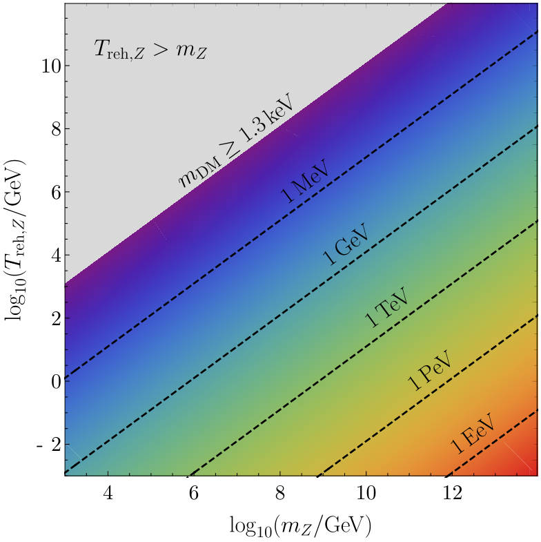
while (3.22) remains unchanged, except for the replacement . Note that for moduli with masses , the lower bound on the DM mass is , on the range of electroweak-scale DM candidates such as the lightest neutralino. Moreover, the late decay of would ensure that the non-thermal phase space distribution (3.18) remains imprinted into this relic. This is due to the fact that most of the DM is produced around , well below the corresponding thermal decoupling (freeze-out) temperature. Fig. 6 shows the limit (3.26) in the mass vs. reheating temperature plane, excluding the model-dependent region. Note the wide range of values for .
We emphasize that this kind of constraint must be accounted for in any discussion regarding DM production in non-standard thermal histories, with an intermediate matter-dominated epoch between the end of reheating and BBN [98, 99, 100, 101, 102, 103, 104]. For a sufficiently large branching ratio of to , this non-thermal production can dominate over DM freeze-out, which would have occurred during the modified expansion history. We finally mention that it is typical of the decay of a modulus into dark matter to occur in two stages, , where is an intermediate unstable particle, such as the gravitino. This scenario is studied in detail in Section 4.2. As we show there, although the phase space distribution of and differ noticeably in their shape, the rescaled bound on is only corrected by an factor in some regimes.
Our main focus in this section is instead stabilized moduli: scalar condensates that oscillate and subsequently decay in the early Universe, while never dominating the energy budget of the Universe [105, 106, 107, 108, 109, 110, 111, 112, 113, 114, 115, 116, 117, 118, 119, 120, 121, 122, 123]. Without modifying inflation [124], this is typically achieved in model-building by introducing additional interactions that rise the mass of the modulus, increasing its decay rate, and by decreasing the amount of initial misalignment.
It is important to realize that for a subdominant decaying scalar, the post-inflationary background dynamics will be determined by either the oscillating inflaton, or by its redshifting relativistic decay products. Therefore, it is necessary to distinguish between three different scenarios: (a) the modulus begins oscillating and decays during reheating, (b) the modulus begins oscillating during reheating, but decays during radiation domination, or (c) the modulus oscillates and decays during radiation domination. We now proceed to determine the phase space distribution in all three cases, to subsequently determine the Ly- bounds and the corresponding phenomenologies. As we discuss below, the observed DM abundance can be obtained from the decay of a stabilized modulus when its energy density is much smaller than that of radiation.
3.2.1 DM phase space distribution
Case a: Oscillation and decay during reheating ()
We begin by studying the scenario in which the field begins its oscillations during the matter-dominated reheating, and fully decays before the end of reheating. Given that we follow the decay of a classical condensate, its distribution function will be of the form , where is the modulus number density (see Eq. (A.3)), and hence the DM distribution will be given by (3.5), upon replacing . The solution of Eq. (3.6), necessary to determine the cosmic-time dependence of , can be found in a straightforward way, and is given by . Moreover, the number density of the decaying is found by integration of (3.7), again replacing ,
| (3.27) |
Here the subindex ‘osc’ refers to the beginning of the oscillation of , which occurs at . Assuming, as we did for the inflaton, a quadratic minimum for the potential of , we can write , where denotes the value of at the initial misalignment. Straightforward substitution gives then
| (3.28) |
In analogy to the inflaton case, we estimate the decoupling time to be . The effect of any subsequent production is to populate the exponential tail of the distribution. Hence, in what follows we evaluate the distribution at this decoupling time, and disregard the effect of the Heaviside function. Moreover, we will always work in the limit when , as is the case even for stabilized moduli.
To evolve the distribution at later times we make use of the decoupled-regime solution (A.6). Note that in order to apply it we need to account for the redshift that occurs from the decay of to the end of reheating, and the subsequent redshift from the end of reheating to present times. Since
| (3.29) |
we can finally write, at late times,
| (3.30) |
where
| (3.31) |
and
| (3.32) |
Fig. 7 shows the form of this rescaled distribution (blue, solid curve). The low momentum power-law dependence and the exponential tail are evident. Clearly, this distribution is of the form (2.27) with and .
Case b: Oscillation during reheating, decay after reheating ()
Let us now consider the case for which starts oscillating during reheating, and its decay is not completed until the subsequent radiation domination. It is crucial to notice that when this occurs there are two possible solutions for Eq. (3.6),
| (3.33) |
Here we have assumed for simplicity a sharp transition from matter to radiation domination at , with in the former case and in the later case. This approximation necessarily leads to a discontinuity in the Hubble parameter, which will translate into a discontinuity in the distribution function . This is nothing but an artifact of our approximations, and it has minimal phenomenological consequences as we will show below.
For we have . In this case we write the number density of as follows,
| (3.34) |
and
| (3.35) |
On the other hand, if , . Therefore,
| (3.36) |
and
| (3.37) |
By substituting into (3.5) and evaluating at we obtain the distribution at decoupling. Moreover, noting that in this case the redshift occurs in the absence of intermediate entropy production, we can finally write the form of the distribution at late times in the following simplified way,
| (3.38) |
with
| (3.39) |
where denotes the background temperature at the moment of decay, and
| (3.40) |
This rescaled distribution is shown in Fig. 7 for . The analytical expression (3.40) is shown as the light green dot-dashed curve. It shows the different scaling with for and , with a jump at . As we mention above, this discontinuity is an artifact of our approximations, demonstrated by the dark green, dotted curve in this same figure, which shows the fully numerical solution, which interpolates smoothly between the two regimes. Note that for the fitting function (2.27) fails to accurately describe the distribution. Nevertheless, for , it accurately describes the DM phase space distribution for any , with and .
Case c: Oscillation and decay during radiation domination ()
For the last case we assume that the beginning of the oscillation of is delayed beyond the end of reheating, due to a rapidly decaying inflaton, a relatively light , or a combination of both. The absence of a matter-radiation crossover during oscillations, and of an intermediate entropy production regime, make this analysis straightforward. The solution of (3.6) is simply given by , and from it we obtain the following expressions for the number density in ,
| (3.41) |
and the Hubble parameter,
| (3.42) |
Substitution into (3.5) and (A.6)
| (3.43) |
with and
| (3.44) |
The resulting distribution is trivially of the form (2.27), and is shown in Fig. 7 as the red, dashed curve.
3.2.2 Power spectrum and Ly- constraints
The analytical determination of the phase space distributions in all cases allows us to map the WDM Ly- constraints to the production of DM from moduli decay. The main hurdle consists in the evaluation of the second moment of the distribution in the case when the oscillation and the decay of occur in different epochs,
| (3.45) |
Here denotes the exponential integral function. Nevertheless, we find the following to be a good approximation,
| (3.46) |
As expected, the limit on the DM mass is weakened if decays during reheating, relative to decay during radiation domination. In this case, DM is cooled down in two stages: from the redshift from to and from the subsequent redsift from the end of inflation to the present epoch.
Fig. 8 shows the transfer function for stabilized modulus decay compared to WDM with and , for the three cases discussed in this section. The overlap between NCDM and WDM is good for all shown scales, albeit a slight shift can be observed for . As Fig. 3 shows, the relative difference is in all cases . The DM masses are taken from (3.46), where the modulus mass and decay temperature are in turn chosen to be and for case (a), and for case (b), and and for case (c). These values are motivated by our discussion of the phenomenology of a strongly stabilized Polonyi-like modulus, in Sec. 3.2.3. For these choices of the mass and decay temperature both the Lyman- bound and the closure fraction bound are saturated (see Fig. 9).
3.2.3 Relic density and phenomenology
We now consider the possible phenomenological consequences of the Ly- bound on found above. We first determine the DM relic abundance from stabilized moduli decays. Integration of Eqs. (3.30), (3.38) and (3.43) provides the following expression for the late-time DM number density,
| (3.47) |
As mentioned above, the discontinuity in the phase space distribution for is not inherited by the number density, justifying our approximations. We emphasize that our results are valid only if the field does not dominate the energy budget of the Universe at any time. For the first scenario, decay before reheating, this is ensured for , since if then it will continue being so until the decay of . For the other two cases we must ensure that the energy density in radiation, , is always greater than . Since the oscillating modulus redshifts more slowly than the background radiation, it is sufficient to enforce this condition at -decay. With and , we can evaluate the scale factors explicitly to obtain that
| (3.48) |
This ratio must be if our present analysis is to be valid. Otherwise, a -dominated epoch occurs, and the bound (3.26) applies. Note that for a branching ratio , the condition is necessary to obtain the observed DM abundance. For example, saturating the Ly- bound (3.46) one obtains for cases b and c.
We now consider as a proof-of-concept example a particular realization of modulus stabilization, corresponding to a strongly stabilized Polonyi field1111 11 The Polonyi field, if left unstabilized, is an example of a problematic modulus for BBN that can arise in supergravity [125, 126, 127, 128, 129]. This field, responsible for the breaking of supersymmetry, communicates with the SM through Planck-suppressed interactions. It is also relatively light: its mass of the order of the gravitino mass, which in turn is parametrically related to the scale at which supersymmetry is broken. Moreover, typically its initial misalignment is . in supergravity, stabilized by the non-minimal addition to the Kähler potential [107, 108, 109, 110, 111, 118]. For our purposes it is sufficient to note the following values of the Polonyi modulus mass, its misalignment, and its decay rate
| (3.49) |
Here is the gravitino mass for this particular case of gravity-mediated supersymmetry breaking, and . Hence, the entropy production problem is averted by simultaneously increasing the mass well above the electroweak scale, by reducing the misalignment to deep sub-Planckian values, and by enhancing the decay rate. The dominant decay channel of is to two gravitinos, which then subsequently decay into the lightest neutralino. Although in this example this decay chain implies that the (rescaled) DM distribution will not be exactly given by the , the scaling of the Ly- constraint will be maintained up to corrections (see Section 4.2).
Fig. 9 shows the allowed parameter space for as a function of the quantity , where . Here includes the inflaton-matter (or radiation) couplings and the phase space factors of the width. This parametrization is chosen to coincide with that of [118], and is inspired by the Planck-suppressed decays which are a generic feature of supersymmetric reheating (see e.g. [130, 119]). As it can be seen, when the stabilization scale is close to the Planck scale, the modulus ceases to be strongly stabilized, and it dominates the energy budget of the Universe after inflation. This is averted for
| (3.50) |
In this figure we have also shown the domain restricted by Ly- observations. We observe that it extends the disallowed region (due to entropy production) by about an order of magnitude in . Its boundary, and the orange line for which the observed DM abundance is obtained for , are determined through the following expression,
| (3.51) |
In the parameter range shown in the figure, the Ly- and DM abundance constraints are simultaneously saturated for
| (3.52) |
assuming . For , , c.f. Fig. 8. We finish by noting that for this particular stabilization scenario, the Ly- constraint is irrelevant compared to the requirement that assuming electroweak-scale LSP masses. Nevertheless, the power spectrum bound may be relevant for alternative constructions in which the modulus mass and the DM mass are independent.
4 Freeze-in via decay
In the previous section we considered the production of DM from the decay of the spatially homogeneous condensate. We now extend our discussion to decays of particles with distributions populated above the zero-momentum mode. Specifically, we will determine the phase space distribution and the mass lower bound for DM produced from the decay of a thermalized relic, and from the decay of a non-thermalized inflaton decay product. As in all cases, we will assume that DM interactions are sufficiently suppressed to prevent it from reaching kinetic and/or chemical equilibrium. For this reason we dub this scenario freeze-in through decays [6].
4.1 Thermal decay
4.1.1 DM phase space distribution
Let us first consider the decay of a population of particles in thermal equilibrium, which decays during radiation domination totally or partially into DM. For definiteness we will assume again that the unstable particle, denoted here by , decays to DM, , via a two-body channel, .
The integration of the corresponding collision term can be performed in complete analogy to the inflaton decay scenario (see Eq. (3.1.1)). Noting in particular that, for a two-body decay, the unpolarized amplitude squared is determined solely by the masses of the initial and final state particles, we can write
| (4.1) |
where
| (4.2) |
Note that up to this point no assumptions have been made regarding the form of . For our exploration of the decay of a thermalized relic into DM, we can assume that , and substitute a thermal Bose-Einstein (BE) of Fermi-Dirac (FD) form for ,
| (4.3) |
Substitution into (4.1) yields the following collision term,
| (4.4) |
Disregarding the inverse decay process, and recalling the relation between time and temperature during radiation domination,
| (4.5) |
the solution of the transport equation (3.1) is a straightfoward application of the freeze-in solution (A.4). After some algebraic manipulation, the DM phase space distribution can be cast in the following form [131, 132]
| (4.6) |
Such expression is valid up to the decoupling temperature below which the dark matter production from the thermal bath is negligible.
A closed form for for either bosonic or fermionic is not available, and (4.6) must be integrated numerically. These distributions are presented in Fig. 10 in the limit when , by neglecting the temperature evolution of the effective degrees of freedom during production, in terms of the rescaled distribution
| (4.7) |
Here , noting that (4.5) can be extended up to recombination, where . The continuous red (blue) curve corresponds to a decaying fermion (boson) . It is worth noting that the difference between the two curves is relatively small, which suggests that a phenomenological Maxwell-Boltzmann-like fit could describe these distributions. Indeed, Fig. 10 also shows two dashed curves which correspond to the following fitting functions,
| (4.8) |
Save for the fitting factors, the functional form for this expression may trivially be obtained from (4.6) in the Maxwell-Boltzmann limit, for which [133, 134, 72]. Worth noting is the mapping of the exponential tail from the thermalized progenitor to the daughter particles. Nevertheless, the low-momentum behavior is different, manifesting the lack of thermal equilibrium in the sector. This distribution is of the form (2.27), with .
4.1.2 Power spectrum and Ly- constraints
The fact that the phase space distribution of is quasi-thermal suggests that the power spectrum should match the one of WDM. Fig. 11 attests the reliability of this matching. The leftmost set of curves shows the transfer functions for the thermal decay cases with BE or FD initial states with masses determined by Eq. (2.25), which in this case corresponds to the following rescaled bound,
| (4.9) |
Here ‘fit’ stands for both the FD and BE approximations (4.8), which differ only by a -independent numerical factor. The overlap of these transfer functions with the WDM result is evident in the whole range of scales shown in the figure, the relative deviation being at (see Fig. 3). In Fig. 11 we also show the form of if we consider a smaller DM mass, and ignore the difference in statistics. In this case, all three curves shift to the left, as expected, but the difference between them remains small. As mentioned earlier, this is the result of the relatively minimal dependence of on the spin of the decaying particle .
4.1.3 Relic density and phenomenology
In addition to the power spectrum constraint on the mass discussed above, one must address the limit from the DM abundance which determines the normalization of the distribution function. Integration of gives the following expression for the DM number density at late times, ,
| (4.10) |
Correspondingly,
| (4.11) |
Except for the number of degrees of freedom, which we consistently normalize to the SM value, the normalizations chosen in the previous equation are inspired by the decay of thermalized supersymmetric particles into light DM candidates, such as the Higgsino axino + Higgs production process in -parity violating DFSZ models [135, 136], for which
| (4.12) |
with the -term parameter , and the Peccei-Quinn scale . Similarly to the inflaton decay case, a mass-independent constraint on the branching ratio to DM from the decay of the thermalized could be derived. Nevertheless, this bound would not be universal, as the mass and width of are model dependent, as opposed to the inflaton decay case (see Eq. (3.22)).
4.2 Non-thermal decay
4.2.1 DM phase space distribution
Let us now assume that the particle whose decay produces the DM interacts very weakly with the SM and was produced via inflaton decay, but does not reach thermal equilibrium. Unlike in the previously studied thermal case, this particle cannot be assumed to be produced abundantly in the thermal plasma during the decay of the latter, Therefore, in principle the imprint that its decay leaves on its phase space distribution must be taken into account.
Disregarding the effect of Bose enhancement/Pauli blocking, and the inverse decay process, the Boltzmann equation satisfied by this non-thermal unstable relic is given by [137]
| (4.13) |
This equation can be exactly solved in the relativistic and non-relativistic regimes. In both cases the decay of proceeds exponentially in time. For this reason we will be content to approximate the evolution of as that of a free-streaming particle until its sudden decay, which occurs at
| (4.14) |
Here denotes the Hubble parameter at the time when becomes non-relativistic. We have estimated the effective lifetime as the inverse of the mean prefactor in the right-hand side of (4.13) [138].
With the previous arguments in mind, for we write the collision term for (4.1) as
| (4.15) |
where the distribution for inflaton decay products , given in terms of the 3D momentum magnitude, was defined in (3.16). In this expression stands for the branching ratio of the decay from inflaton to . Substitution into the general freeze-in solution (A.4) gives
| (4.16) |
where . The ratio
| (4.17) |
quantifies how relativistic the distribution for is at a given moment of time. In particular, we define
| (4.18) |
Extending the solution past we can write
| (4.19) |
where
| (4.20) |
Here and are the same as in (3.16) and (3.17). The rescaled distributions and can be computed by making use of the fit approximation (3.18) for . We obtain
| (4.21) | ||||
| (4.22) |
where denotes the upper incomplete gamma function.
The DM phase space distribution corresponding to the decay of a non-relativistic particle is shown in Fig. 12 as a function of and . The solid black line shows the result of the numerical integration of (4.20). The distribution grows with an almost linear universal envelope, independent of the decay rate of , until , at which point the distribution sharply decreases. This non-universality of the cutoff prevents us from constructing a reasonable fit approximation of the form (2.27) for generic values of . In the same figure, the orange dashed lines show the analytical approximation (4.21), which as can be seen is equivalent to imposing a hard cutoff at on the universal envelope.1212 12 The numerical distribution can be well fitted by substituting the function in Eq. (4.21) by a logistic function.
Fig. 13 shows the numerically computed relativistic distribution as the solid black curve, and the analytical approximation given by (4.22) as the orange, dashed curve. In the same figure a ‘fit’ approximation of the form (2.27) is also shown. This approximation is obtained by mimicking the asymptotic behavior of the gamma function at large and small , while preserving the normalization, and is given by
| (4.23) |
It is worth noting that in this case the Gaussian tail is of the same form as that of the parent unstable particle. It is important to emphasize that this distribution is obtained in the limit , as we discuss below.
Fig. 14 shows the form of the function , defined in Eq. (4.20), for several values of , ranging from to 10. Here we can appreciate the transition between the relativistic and non-relativistic decay cases. In all cases the phase space distribution peaks at , with a positive skew for a relativistic , and a negative skew for non-relativistic . For the analytical approximation (4.22) describes well the exact distribution for . For , the non-relativistic approximation (4.21) is in turn a good fit for the exact distribution for .
4.2.2 Power spectrum and Ly- constraints
For the distributions that we have derived, we can make use of (2.25) to determine the rescaling of the bound on the DM mass. For the case of a relativistic (R) decay we find that
| (4.24) |
while for the non-relativistic (NR) case,
| (4.25) |
The behavior is only correct for large but remains a reasonable approximation for . We note here that the lower bound on the NCDM mass can be many orders of magnitude larger than the corresponding WDM bound, and it increases as the reheating temperature is decreased. This is expected, as in this case the parent particle is produced from inflaton decay (see Sec. 3.1.2). The difference between the numerical and analytical results is minimal, consistent with the agreement between both curves in Fig. 12 and Fig. 13. However, the fit approximation for the relativistic case provides a relatively poor approximation to the bound, overestimating it by a factor of .
Figs. 15 and 16 show the results of the numerical evaluation of the transfer functions with CLASS [44, 45], and their comparison with the WDM case.1313 13 For the relativistic case, the small disagreement between the numerical transfer function with values from Eq. (4.24) and the corresponding WDM spectrum is also attributed to the sharp drop of the phase space distribution for , akin to a low-momentum cutoff. Such a cutoff results in a loss of numerical precision if reasonable computation times are required. For the two sets of curves shown in each figure, we use the rescaled Ly- bound (4.24) or (4.25). For the leftmost set we take and , while for the rightmost set we consider and . For the decay of a non-relativistic particle, a comparison is made between the three different choices for and . Note the overlap between the three curves, with a relative difference of (see Fig. 3, where the relative difference is plotted as a function of for ). For the decay of a relativistic particle, the agreement between the numerical and analytical results can be immediately appreciated, as well as the difference between these and the result of using the fit approximation (4.23) for the DM distribution.1414 14 The analytical expression of Eq. (4.21) is not represented in Fig. 15 as the sharp -function cannot be handled properly with CLASS as it requires the distribution function to smoothly decrease at large . Even more evident though is the difference of the NCDM transfer functions with respect to the one for WDM, of around at , c.f. Fig. 3. For the relativistic case, the distribution has a very non thermal shape, monotonically decreasing with , resulting in a power spectrum that, although not too dissimilar from the WDM case, exhibits in the figure an appreciable difference from it.
4.2.3 Relic density and phenomenology
The present relic abundance of DM is obtained from integration of (4.19). To do this we make use of the (numerical) result
| (4.26) |
At the number density has the form
| (4.27) |
Note that both expressions agree up to a different power of the number of relativistic degrees of freedom. This agreement is to be expected, as the total number of the decaying particle and its decay product must be a constant in a comoving volume. Considering for definiteness the case of a relativistic decaying particle, we determine that the present abundance is given by
| (4.28) |
As expected, is independent of the properties of , and corresponds simply to a re-scaling by degrees of freedom of the inflaton decay result (3.21).
Given this result, a universal lower bound on can be obtained, in full analogy with the inflaton decay scenario. Let us discuss it in the context of a specific model. Consider the decay chain inflaton gravitino LSP (lightest supersymmetric particle), which is generically present in supersymetric models of inflation with supersymmetry breaking mediated gravitationally [139, 140, 141, 142, 143].1515 15 In typical gauge-mediation scenarios, the gravitino can be very light, and is produced through thermal freeze-out, thus being an example of WDM [144, 145, 146, 147, 39]. Assuming a minimal supersymmetric extension of the Standard Model (MSSM), the decay rate of the spin-3/2 gravitino is [148]
| (4.29) |
Generically, . Substitution into (4.24) and (4.28) leads to the following absolute constraints on the branching ratio of the decay of the inflaton into gravitinos, independent of the DM mass: For non-relativistic decaying particles, and
| (4.30) |
while for relativistic decaying ones, and
| (4.31) |
In this (MSSM) scenario, the excluded DM masses span a phenomenologically interesting region in the parameter space of the model, as shown in Fig. 17. The exclusion region corresponds to
| (4.32) |
These bounds are or the order of the electroweak scale, and are comparable to collider and direct detection limits [149, 150]. Note that for a model-fixed LSP mass, the Lyman- constraint puts a bound on the inflaton-matter couplings. For , are excluded.
A straightforward computation shows that independently of the mean momentum of the decaying gravitino, the decay occurs at temperatures at which the LSP can be safely assumed to be decoupled from the thermal plasma, and hence preserves its non-equilibrium phase space distribution.
5 Ultraviolet freeze-in via scatterings
In this section we consider the production of light DM from scatterings in the primordial plasma. We will restrict ourselves to processes, for which the integrated effective cross section is assumed to be of the form
| (5.1) |
where is an integer and is the Mandelstam variable, related at high energies with the center of mass energy by . Although for non-negative this cross section naively violates unitarity at high energies, we assume that it merely corresponds to the low-energy effective description of a UV-complete model. The energy scale can be thought to be parametrically related to the mass of a heavy mediator. The suppression by guarantees that the primordial abundance is determined by forward processes (plasma DM) rather than by annihilations. Therefore, Pauli-blocking/Bose-enhancement for can be safely disregarded, and in the absence of other interaction channels, never reaches thermal equilibrium with the plasma. Thus, freeze-in is realized [6, 151].
Assuming no post-reheating entropy production (that is, a standard thermal history), particle production is dominated by temperatures if . This is referred to as ultraviolet (UV) freeze-in [152, 153, 49]. Moreover, for , and for a sufficiently large reheating temperature, we can safely assume that both the parent scatterers and the produced DM are ultrarelativistic at the time of production,1616 16 This justifies disregarding any dependence on thresholds. For , the masses of the scatterers play an important role to determine the lower bound on [71, 72]. if the former are in thermal equilibrium. If the parent scatterers are not in equilibrium at production time, the condition that their masses are suffices. Here we will consider both scenarios.
In order to evaluate the necessary collision terms for thermal and non-thermal production, we need to make assumptions regarding the form of the scattering amplitude. Its dependence on the angles (or Mandelstam variables ) involved in the scattering varies between different microscopic descriptions of the process. We will assume that for the scattering process , the mean, unpolarized squared scattering amplitude can be parametrized in the following way,
| (5.2) |
Integration with respect to the two-particle phase space recovers (5.1). For a different combination of , our results will generically only differ by numerical factors, which can be absorbed into the value of .1717 17 Exceptions include those cases in which finite-temperature in-medium effects are necessary to regulate infrared divergences, which arise from the exchange of massless mediators. Thermal axion production and gravitino production in low-scale supersymmetry are included in these cases [154, 155, 156, 157, 158, 159].
Under the freeze-in assumption, and with the square amplitude given by (5.2), the collision term for the production of can be written as follows,
| (5.3) |
The integration of this collision term for arbitrary can be easily done following the steps of [155, 160]. We detail these steps in Appendix A.2. As a result, we obtain Eq. (A.13), which will be the starting point of our discussion of thermal and non-thermal UV freeze-in.
5.1 Thermal freeze-in
We begin by applying the general solution (A.13) to the production of DM from thermalized scatterers, i.e. with Fermi-Dirac or Bose-Einstein distributions. As stated earlier in this section, we focus on UV freeze-in, for which the bulk of the DM relic abundance is produced during reheating. Thermal production during reheating is the dominant production channel in the absence of significant direct inflaton DM decays for in (5.1). Moreover, for higher , thermal production can dominate over non-thermal effects if the parent scatterers that couple to the dark sector are not directly produced from inflaton decay (see e.g. [161]). Given the need to compute the integrals in (A.13) in a case-by-case basis for scatterers outside of the Maxwell-Boltzmann limit, we will focus on the lowest even values of , namely . In doing so, we will recover the results of [153], showing that for , thermal production is dominated by the highest temperature during reheating, ??.1818 18 More precisely, denotes the maximum temperature of the Universe after the thermalization of the primordial plasma during reheating. In the regime where non-perturbative particle production is the subdominant decay channel for the inflaton, this , although it is smaller than the value that it would naively have assuming instantaneous thermalization [162, 163, 164].
5.1.1 DM phase space distribution
For any , the computation of the innermost integrals in (A.13) can be performed analytically (in terms of polylogarithmic functions) if the initial states have the form fermion+fermion (FF), fermion+boson (FB) or boson+boson (BB). The outermost integral is however more challenging, and we compute it numerically. The result can be written as
| (5.4) |
where we have simplified the notation assuming that the DM particles are ultrarelativistic at production, and where the functions are shown in Fig. 18 for the four values of that we consider. In the Maxwell-Boltzmann limit, . This collision term can now be substituted into the general solution (A.4) of the transport equation (3.1). In order to translate the time integral into a temperature integral, we make use of an approximate solution for the Friedmann-Boltzmann system (3.7)-(3.9), which for gives
| (5.5) |
and [153]
| (5.6) |
We have defined here as a function of up to an numerical factor that we denote by .1919 19 The factor depends on how the transition between matter and radiation domination at the end of reheating is described, which complicates the analytical determination of . Extrapolating Eq. (5.6) to yields , while substitution of at in Eq. (3.9) gives . Numerical solution of (3.7)-(3.9) reveals that at (inflaton) matter-radiation equality. For convenience we keep unspecified. Straightforward algebraic manipulation reveal the following form for the DM phase space distribution at the end of reheating,
| (5.7) |
Disregarding the residual production of DM for , we can extend this solution by means of the free streaming expression (A.6) with . Hence, at late times we can finally write
| (5.8) |
where
| (5.9) | ||||
| (5.10) |
| Scenario | Prefactor | ||||
|---|---|---|---|---|---|
| BB | 0.88 | -0.70 | 1.13 | 1.00 | |
| FB | 0.58 | -0.51 | 1.10 | 1.00 | |
| FF | 0.38 | -0.29 | 1.11 | 1.00 | |
| BB | 1.76 | -0.51 | 0.91 | 1.00 | |
| FB | 1.42 | -0.42 | 0.90 | 1.00 | |
| FF | 1.14 | -0.33 | 0.90 | 1.00 | |
| BB | 5.35 | -1.79 | 0.06 | 1.98 | |
| FB | 4.85 | -1.79 | 0.06 | 2.04 | |
| FF | 4.41 | -1.79 | 0.05 | 2.10 | |
The functions for are shown in Fig. 19. In these three cases the integral in (5.9) is dominated by the lower limit: production is peaked at [153]. Therefore the approximation can be taken, implying a loss of dependence on the maximum temperature of the relic density. In all three cases, and for all three different scatterer configurations, the low- part of the distribution grows as a power-law, while the large- part retains the exponential tail of the thermalized parent particles. Hence, phenomenological fits of the form (2.27) can be constructed in all cases, with fit parameters as shown in Table 1. To construct these fits we impose for as the fitted function is already matching well the numerical distributions. However, we left as free parameter for the case in order for the fitting function to accurately describe the distribution. Note that in none of these cases the resulting distribution function fully inherits the FD or BE distribution of the parent scatterers, as it is sometimes assumed [40].2020 20 For , a thermal distribution provides an adequate fit, although worse than a fit of the form (2.27) [165]. It is also worth noting that, although we have not attempted to obtain a closed form expression for the exact distribution, we can compute its integral analytically. Namely, integration of the Boltzmann equation (3.1) with the collision term (5.3) leads to the following evolution equation for the DM number density,
| (5.11) |
Upon integration and evaluation at , the following result is obtained, valid for ,
| (5.12) |
Here is a statistics-dependent function of ,
| (5.13) |
The case is special and must be treated separately. In this case, both limits of integration in (5.9) must be kept to obtain a finite result. This results in a dependence on of the relic density: production is in this case peaked at the maximum temperature after thermalization. This feature manifests itself noticeably in the shape of the resulting phase space distribution. Fig. 20 shows this distribution for two cases, and 50.2121 21 These relatively low values of the temperature ratio are chosen to simplify numerical integrations and the reading of the resulting plots. Additionally, low is required to match the observed DM abundance in the case of light DM. The top panel shows the distributions in a log-linear scale, in order to showcase the significant difference that the value of the temperature ratio makes in the location and amplitude of the peak of . The lower panel of this same figure, in turn, shows the same distributions in a log-log scale, to demonstrate the three different regimes in . For below the peak, the distribution increases as a power law, , while below the peak for . For , the distribution has the expected exponential tail due to the thermal nature of the scatterers. For these reasons we have not presented a fit of the form (2.27) for this () case, as it would inevitably fail to mimic at least one of the three scalings of the distribution. As mentioned in the Introduction, this is one of the cases for which the phenomenological fit is not applicable. Nevertheless, an analytical closed-form solution for the integrated distribution function is available,
| (5.14) |
where for this case,
| (5.15) |
We finish this section with a word on the relevance of quantum statistics. Despite the fact that the use of Maxwell-Boltzmann statistics for the parent scatterers will necessarily lead to errors in the DM and relic abundance, it is instructive to show how much our previous computations are simplified in this limit. As mentioned above, in this case, and therefore the corresponding integration of the collision term proceeds in a straightforward manner to give
| (5.16) |
As is increased, this approximation becomes a better fit for the distributions with the correct statistics, and in fact converges to the FB case. It can also be shown that this convergence is exponential in the case of the relic abundance.
5.1.2 Power spectrum and Ly- constraints
We now proceed to discuss the phenomenological implications of the Ly- rescaled constraints on UV freeze-in. For the low- cases, the WDM rescaling relation (2.25) leads to the following constraints on the DM mass, based on the numerical and fit distributions:
For ,
| (5.17) |
For ,
| (5.18) |
For ,
| (5.19) |
In all cases the agreement between numerics and the fits are evident, since the relative deviations are at most of a few percent. This is further confirmed by the transfer functions shown in Figs. 21 and 22. There, the three possible initial states for each value of are shown together with the corresponding WDM transfer function. In these plots, the leftmost set of curves shows for , built using the fit approximations in each case. The rightmost set of curves, in turn, correspond to , and the DM bound derived from the numerically computed distributions. All results confirm our constraint mapping procedure to a precision , as shown in Fig. 3 for the FF cases.
As we discussed above, the case with needs to be treated separately, due to its dependence on . In this case, the mapping relation (2.25) gives the following rescaling on the DM mass bound, based on the numerically determined phase space distribution shown in Fig. 20,
| (5.20) |
and
| (5.21) |
Fig. 22 shows the form of the linear transfer function for both temperature ratios and all initial configurations, compared to the WDM case. There is a noticeable deviation between the WDM transfer functions and those for this freeze-in scenario, which increases as is increased relative to , correlated with the presence of a longer power-like tail in the distribution. For , this difference is as large as at , as is shown in Fig. 3. It is worth pointing out that the Maxwell-Boltzmann approximation (5.16) can be used to estimate the DM mass bound without the need for numerical computations. From it, we obtain .
5.1.3 Relic density and phenomenology
For , the DM number density and the abundance can be computed analytically by means of (5.11), and result in the following expressions,
| (5.22) |
and
| (5.23) |
For , the late-time DM number density and the present DM relic abundance can be found by integration, and are given by
| (5.24) |
and
| (5.25) |
Similarly to the inflaton decay scenario, the Ly- constraint on the DM mass and the DM relic abundance can be combined, in this case to exclude values of the pairs . Fig. 23 shows the excluded parameter space in the plane, for . To construct this plot we have taken the parameter to be 1, and neglected the contribution from the internal degrees of freedom of the annihilating SM particles and the scattering products. The thickness of the boundary lines, at which the bounds are saturated, corresponds to the difference between the possible initial state quantum statistics. As we discussed earlier, this difference is reduced as is increased. Annihilations with a steeper dependence on the center of mass energy allow for a wider range of values for the scale than processes with a low values of . Notice that this scale cannot be taken much below the inflaton mass by construction. Indeed, in this case the effective-field-theory approach used to describe the DM-SM scattering amplitude would cease to be valid for processes involving the most energetic SM particles produced in the early universe.
The bounds tend to converge for larger values of the reheating temperature. For the special case the maximum temperature of the universe is taken to be the temperature at thermalization, which is dependent on the decay rate and therefore on the reheating temperature, . This functional relation can be obtained by substituting in (5.6) the thermalization time-scale (5.33), which we discuss in more detail in the following section.
It is outside of the scope of our study to provide a detailed account of the implications of our analysis for the many DM models for which the UV thermal freeze-in mechanism is the dominant production channel. Moreover, for many of these constructions, the physics that gives rise to the suppression by the scale for the cross section leads to electroweak-scale DM candidates, as in Grand Unification constructions () [19, 20], or super-heavy DM candidates, as is the case of gravitino DM from high-scale supersymmetry models () [166, 167, 168]. Nevertheless, we now identify a few scenarios for which is viable for the various thermal freeze-in cases that we have discussed above. A well known example of light DM with freeze-in is axino DM, with a production cross section suppressed by the Peccei-Quinn scale, [169, 170, 171, 172, 173, 174, 175, 136].
Light DM produced from UV freeze-in can take the form of a spin-3/2 particle (the “raritron”) [161]. In a SM extension that contains a right-handed and/or sterile neutrino with mass , the following Lagrangian determines the DM interactions,
| (5.26) |
where denotes the raritron, the field strength tensor, and the SM Higgs doublet. When the term proportional to dominates raritron production, the processes , and populate the DM energy density during reheating, with , i.e. . On the other hand, if the coupling dominates, , that is . We elaborate on the interplay between thermal and non-thermal effects for the case in Section 5.2.3.
In scenarios inspired by modified gravity, SM-DM interactions can be mediated by a massive spin-2 particle [23, 24],
| (5.27) |
where is the SM (DM) energy-momentum tensor and some energy scale. Scalar, fermion or vector light DM can be produced through thermal freeze-in during reheating. For a heavy mediator, , , realizing . For a lighter mediator, , , i.e. .
We finish this section by briefly addressing the more exotic scenarios, arising e.g. in vector non-Abelian DM constructions with SM-DM interactions mediated by a heavy [21]. For these cases, (5.16) is a good approximation for the phase space distribution. A straightforward computation reveals that the “plateau” behaviour observed for is also present, with and below and at the plateau, respectively. It can be verified that the lower bound on the DM mass is suppressed with respect to the WDM case by powers of the ratio of the reheating temperature and the maximum temperature,
| (5.28) |
These limits must be complemented with the DM density bound, which in these scenarios reads
| (5.29) |
Note the inteplay of the scale and the maximum and reheating temperatures. The requirement that narrows down the available parameter space for a given , disfavoring DM masses near the bound (5.28).
5.2 Non-thermal freeze-in
In the previous section we have addressed the production of DM in UV-dominated freeze-in models, exploiting the fact that reheating is not an instantaneous process, as it involves a continuous transfer of inflaton energy density into its relativistic decay products. The thermalization process, during which elastic and inelastic scatterings in the primordial plasma bring it into kinetic and chemical equilibrium is also non-instantaneous. In typical perturbative reheating scenarios, thermalization is reached after the end of inflation, but well before the end of reheating, if it is mediated by (SM) gauge interactions [162, 163, 164]. As it was found in [49, 176], even if this non-thermal (or “pre-thermal”) window may be relatively narrow, the bulk of the DM abundance may be produced during this time interval, provided that the production scattering cross section is a sufficiently steep function of energy. More concretely, if in (5.1), the inflaton decay products, with momenta , can copiously produce DM particles, which will eventually dominate the DM density budget despite their dilution by entropy production during the late stages of reheating. In what follows we will consider only the lowest case with even for which this pre-thermal production can dominate, that is .
5.2.1 DM phase space distribution
Assuming that the initial state particles necessary for DM production are produced directly from inflaton decay, their distribution before thermalization can be approximated by Eq. (3.11). This distribution is highly non-thermal, peaked at momenta , with a cutoff at . Nevertheless, due to its power-law nature, it allows a closed form computation of the collision term. For the interested reader, this calculation is presented in Appendix A.3. Moreover, integration of the transport equation by means of (A.4) can also be performed analytically. The resulting phase space distribution at the thermalization time , when the interactions between the scatterers become sufficiently efficient to bring the plasma into thermal equilibrium, is given by
| (5.30) |
where
| (5.31) |
Fig. 24 shows the momentum dependence of the rescaled distribution for the non-thermal freeze-in scenario. At low momentum the DM inherits the power-law dependence of the parent scatterers, c.f. Eq. (3.11). At higher momentum, , a peak in the distribution appears, and for larger momenta the distribution decays faster than an exponential, finally vanishing at . Although we have at our disposal the exact form for the phase space distribution, it is nevertheless instructive to verify that a fit of the form (2.27) can be constructed:
| (5.32) |
This fit is also shown in Fig. 24.
In order to extend the distribution to later times, we require to know the thermalization time-scale and the expansion history from to . Denoting by the gauge coupling responsible for the thermalization of the (SM) inflaton decay products, the thermalization time-scale can be approximated as follows [162, 163, 164]
| (5.33) |
With the scale factor during reheating being we finally have
| (5.34) |
for . Here
| (5.35) |
and was defined in (5.6).
5.2.2 Power spectrum and Ly- constraints
The analytical expression for the DM phase space distribution for non-thermal freeze-in allows us to obtain the rescaled bound of the DM mass from Eq. (2.25). It is given by
| (5.36) |
where, for completeness, we have also included the bound obtained by using the fit approximation (5.32). Their agreement is excellent. Note here that, for the fiducial values and , the lower bound on the DM mass is one order of magnitude smaller than for WDM, and can be decreased by increasing the reheating temperature. Unlike the case of production from inflaton decay, where a hot spectrum could be obtained for large masses due to a reduced momentum redshift and a large momentum at production, in this case a colder spectrum is obtained due to the redshift that occurs between and , in addition to the redshift from to ; despite having at production.
Fig. 25 shows the transfer function for non-thermal freeze-in corresponding to the rescaled DM masses (5.36). Two sets of parameters are explored, one with and (right), and with and (left). Both cases overlap with the reference WDM for all the range of scales shown, with a relative difference below the percent level (c.f. Fig. 3), once again demonstrating the validity of our rescaling program.
5.2.3 Relic density and phenomenology
The DM number density at late times can be easily calculated given that
| (5.37) |
It is given by the following expression, for ,
| (5.38) |
In turn, the DM abundance has the following form,
| (5.39) |
If the decay of the inflaton to the parent scatterers is subdominant with respect to other channels, the previous expression is reduced by the corresponding branching ratios, .
Combining the DM abundance and mass constraints, we can obtain a bound on the reheating temperature analogous to that for thermal freeze-in. In this case, the bound takes the form
| (5.40) |
As we mentioned in Section 5.1.3, freeze-in with is realized for scattering processes involving neutrinos for the spin-3/2 raritron. With the interactions mediated dominantly by the first term of (5.26), and under the assumption that the inflaton predominantly decays to Higgs bosons, the thermal and non-thermal relic abundances can be written as
| (5.41) |
and
| (5.42) |
For the DM energy density is mostly comprised of non-thermally produced raritrons. Fig. 26 illustrates the different domains in the parameter space where freeze-in production can occur either thermally or non-thermally. For definiteness we have fixed the branching ratio to neutrinos to . We observe that for the production is dominated by thermal effects, which are most efficient around . The Ly- bound in this case is independent of the inflationary parameters, and it is given by (5.19). On the other hand, for lower reheating temperatures freeze-in occurs before thermalization is complete. The limit on the mass is therefore given by (5.36) and is -dependent. We finally note the region in the botton right corner, in which the unstable raritron would decay faster to photons than experimentally allowed. We refer the interested reader to [161] for further details.
6 Light, but not too light, dark matter
In our exploration of non-equilibrium DM production scenarios we have focused on WDM mimickers: DM which is sufficiently relativistic during structure formation to leave a detectable imprint in the matter power spectrum at scales below their free-streaming horizon, yet heavy enough to be indistinguishable from CDM at late times. Such a DM candidate may, in principle, contribute significantly to the number of effective relativistic species, , at recombination or BBN. It is for this reason that we evaluate this contribution in this section. Well after DM decoupling, the total energy density in the Universe can be written as
| (6.1) |
where denotes the energy density of photons, is the effective neutrino temperature, after electron-positron annihilation, and the dots include all other contributions to , such as that of baryons. In the SM, . In order to determine the contribution of DM to one could naively think of placing its energy density inside the brackets. However, the equation of state of our DM candidates lies in between that for radiation and pressureless dust (and varies in time). Hence, as it is sometimes done [177, 178, 54], we separate its energy density into relativistic and non-relativistic parts, , and absorb only the former into the factor multiplying in (6.1).2222 22 This (artificial) splitting has the effect of suppressing the mass- and time-dependent contribution to , which, if dominant, would signal the non-relativistic nature of the DM. With this, we can then write
| (6.2) |
The contribution to depends on the ratio . As expected, for a given , decreasing this ratio increases . Hence, the maximal contribution to the number of relativistic degrees of freedom for a given DM scenario is obtained by saturating the Ly- constraint, which by virtue of (2.25) fixes the value of the mass to ratio up to ,
| (6.3) |
where
| (6.4) |
For all the DM production mechanisms that we consider in this work the geometric and arithmetic means of are approximately . The largest value of () is 3.4 (1.7) corresponding to the thermal freeze-in case, while the smallest is 0.3 (0.2) for the non-thermal decay case. With this in mind, we can immediately verify that DM with the lowest allowed mass will be relativistic at , as . Hence,
| (6.5) |
well below the constraining power of BBN computations, for which [179, 180]. On the other hand, at , , so that DM is mostly non-relativistic, and contributes negligibly to , , far below the current and projected detectability thresholds [47, 181, 182]. We can then conclude that for none of the production scenarios explored in this work does DM significantly contributes to the amount of non-photonic relativistic species.
7 Conclusions
We have investigated the imprint on the matter power spectrum at small scales of Non-Cold Dark Matter (NCDM, i.e. a DM species with a non-vanishing equation of state parameter ) produced in an out-of-equilibrium state. The ratio of the matter spectrum for NCDM to that in CDM features a cutoff at large Fourier modes. Rather generically, the cutoff scale, i.e. the free-streaming horizon, depends only on . The Lyman- forest constraint on the Warm Dark Matter mass can be translated into a constraint on , being . By comparing the theoretical value of for a given NCDM model with a non-thermal phase space distribution to , we can map the constraint on to the DM mass in the NCDM model. The key result of this paper, which we have illustrated with many examples, is that our mapping procedure allows to translate the Lyman- bound on to non-equlibrium NCDM scenarios without performing a numerically costly computation of the power spectrum for each model. All that is necessary to obtain the (lower) bound on the DM mass is to determine the present DM momentum dispersion and the first two moments of the corresponding distribution function.
To test our formalism we have considered several NCDM production mechanisms. In all of them, the assumption of DM decoupling immediately after production is implicit, ensuring that its phase space distribution is preserved until later times, up to redshift effects. The scenarios that we have considered correspond to DM production from scalar condensates (inflaton, moduli), thermalized and non-thermalized particles, and thermal and non-thermal freeze-in. In each case we have computed the DM phase space distribution either analytically or numerically by means of the Boltzmann equation and computed numerically the linear matter power spectrum using the CLASS code. We compared our results with the WDM linear power spectrum (assuming a fermionic WDM benchmark candidate), showing a good agreement with our matching procedure on the Lyman- bound on . Our matching procedure is performed with a relative precision of for most of the scenarios whereas for the least precise cases, over the range of Fourier wavenumbers of interest for Lyman- data. Such a precise matching highlights one of our main conclusion that the linear transfer function, for all the cases considered in this work, is essentially controlled by the single parameter .
Phase space distributions. For all but two of the scenarios considered in the present work, we have shown that the DM phase space distribution can be well fitted by a generalized distribution of the form
| (7.1) |
with constant and , as required for the DM number density to be finite. The only scenarios in which this fitting fails are for thermal freeze-in production with a SM-DM scattering cross section and , for DM production from strongly stabilized moduli decay, when the inflaton and modulus decay rates are comparable, and for the decay of a non-thermalized particle with . For the rest of the scenarios the values of the parameters and are summarized in Table 2.
| Scenario | Figure | Section | ||||
|---|---|---|---|---|---|---|
| Inflaton decay | -3/2 | 0.74 | 1.00 | 4 | 3.1.1 | |
| Moduli decay | during reheating | -3/2 | 1.00 | 3/2 | 7 | 3.2.1 |
| after reheating | -1.00 | 1.00 | 2.00 | 7 | 3.2.1 | |
| Thermal decay | -1/2 | 1.00 | 1.00 | 10 | 4.1.1 | |
| Non-thermal decay | non-relativistic | - | - | - | 12 | 4.2.1 |
| relativistic | -5/2 | 0.74 | 2.00 | 13 | 4.2.1 | |
| UV Freeze-in () | BB | -0.70 | 1.13 | 1.00 | 19 | 5.1.1 |
| FB | -0.51 | 1.10 | 1.00 | 19 | 5.1.1 | |
| FF | -0.29 | 1.11 | 1.00 | 19 | 5.1.1 | |
| UV Freeze-in () | BB | -0.51 | 0.91 | 1.00 | 19 | 5.1.1 |
| FB | -0.42 | 0.90 | 1.00 | 19 | 5.1.1 | |
| FF | -0.33 | 0.90 | 1.00 | 19 | 5.1.1 | |
| UV Freeze-in () | BB | -1.79 | 0.06 | 1.98 | 19 | 5.1.1 |
| FB | -1.79 | 0.06 | 2.04 | 19 | 5.1.1 | |
| FF | -1.79 | 0.05 | 2.10 | 19 | 5.1.1 | |
| UV Freeze-in () | BB | - | - | - | 20 | 5.1.1 |
| FB | - | - | - | 20 | 5.1.1 | |
| FF | - | - | - | 20 | 5.1.1 | |
| Non-thermal UV Freeze-in | -3/2 | 2.5 | 2.6 | 24 | 5.2.1 | |
For the decay of a scalar condensate, the form of the distribution is determined by the expansion rate. If the decay occurs during a period with a background equation of state , then at low momentum. On the other hand, the exponential decay of the condensate makes at large momentum. For a stabilized modulus the combination of both regimes results into (7.1).2323 23 Unless its decay occurs close to the end of reheating. For inflaton and non-stabilized moduli, the low momentum part of the distribution is populated during the matter-like oscillations of the field, with , while the exponential tail is populated during the subsequent radiation domination, with .
In the case of thermal decays, the integrated thermal distribution of the progenitor particles leads to an enhanced distribution at low momentum, , while preserving the thermal exponential tail. An analogous effect is present in the decay of a (relativistic) non-thermalized relic produced from the decay of the inflaton. Here the shift to lower momenta corresponds to , while the Gaussian tail is preserved. More interesting is the decay of a non-equilibrated non-relativistic relic. In this case we find that the phase space distribution is skewed toward large momentum, with a sharp cutoff dependent on the inflaton and decaying particle masses and widths.
Thermal freeze-in production during reheating encompasses a variety of scenarios that can be distinguished by the nature of the scattering particles that produce DM, which can be any combination of fermions and bosons, and by the dependence of the production cross section on the center of mass energy. In all cases, the statistics of the scatterers manifests itself mostly as an overall normalization of the distribution function, and only mildly through the shape of the distribution, as it can be seen in Table 2. Moreover, the role of statistics is greatly reduced for a steeper energy dependence of the cross section. Regarding this dependence, for , a shift of the thermal distribution to lower momenta is observed, similar to thermal decays. At , the shift is greater, and the thermal exponential tail is lost. For , the distribution depends now on two scales: the reheating temperature and the maximum temperature after thermalization . The result is a distribution with a peak with a location and amplitude inversely dependent on the ratio , that increases as below this peak, and decreases as for momenta larger than the peak and smaller than , beyond which the distribution acquires an exponential suppression.
If the DM parent scatterers are directly produced from inflaton decay, for the DM relic abundance can be produced prior to the thermalization of the primordial plasma. We considered the case, obtaining a closed form expression for the phase space distribution. At low momentum the distribution inherits the power-law increase of the parent scatterers, , while for a sharp decrease is observed, with .
Ly- constraints. Given the parametrization (7.1), our re-scaling of the WDM Ly- constraint on the DM mass can be written as
| (7.2) |
where denotes the mean DM momentum at present time. The previous expression can be read as follows: the non-thermal shape of the phase space distribution represents, in most cases, an correction to the DM mass bound. It is the overall normalization of the distribution what mostly contributes to increasing or decreasing this bound. This normalization depends on the production mechanism, the mean energy of the parent fields, and the expansion history from DM decoupling to the present epoch.
As it can be expected, for all thermal production mechanisms, the resulting Ly- bound is only mildly corrected with respect to that for WDM. From thermal decays, depending on whether the decaying particle is a fermion or a boson, respectively. For thermal scatterings, we also see a small spread, with for , for , and for . Even for , we obtain for .
For the decay of scalar condensates we find a significant amount of rescaling of the Ly- bounds. For unstabilized moduli or inflaton decay, the constraint is proportional to the field mass, and inversely proportional to its reheating temperature. If we restrict this ratio to be larger than one, we obtain that can be as low as or as large as , as shown in Fig. 6. For an inflaton of mass , for . For stabilized moduli, which by assumption never dominate the energy density of the Universe, the DM mass bound depends on the ratio of the modulus and the background temperature at the time of its decay. If the modulus decays during reheating the mass bound depends also on the ratio of its decay rate to that of the inflaton. This scenario is model dependent. For the stabilized Polonyi example that we discuss in Section 3.2.3, the lower bound on the DM mass ranges from if the modulus decays during radiation domination, to if it decays during reheating.
If DM is produced from the decay of a non-thermalized inflaton decay product, , the lower bound on its mass depends on whether the intermediate particle decays while being relativistic or non-relativistic. In the former case, DM inherits a hard distribution with . The result is a Ly- bound almost identical to that of the inflaton decay case, except for a reduction of by a factor of 3. On the other hand, if the decaying particle is non-relativistic at the time of decay, the phase space distribution of DM is highly non-thermal, and the Ly- bound on its mass depends on the ratio of the decaying mass to the temperature at which it decays, .
When DM is produced from the scattering of non-thermalized inflaton decay products, as in the non-thermal freeze-in case, it also inherits the hard momentum distribution. However, in this case the bound becomes on the thermalization timescale, as the DM momentum can be significantly redshifted away from the thermalization epoch to the end of reheating due to entropy production. Notably, this implies that for this scenario the DM mass bound can be significantly reduced relative to the WDM case. The result is a relatively complicated function of the inflaton mass, the reheating temperature and the gauge coupling that mediates the interactions that thermalize the plasma, as shown in Eq. (5.36). This results in for .
Phenomenological implications. A lower bound on the DM mass can have far reaching consequences for non-equilibrium DM model building. For thermal freeze-out, only sub-keV particle DM candidates can be ruled out from Ly- forest observations. For non-equilibrated DM, the constraint can be powerful enough to rule out DM candidates, and hence SM extensions, above the electroweak scale.
In the case of inflaton decay, the wide range for means that the suppression of structure at small scales can in principle occur for DM masses well above the electroweak scale if the reheating temperature is sufficiently low. Moreover, combining the power spectrum and DM relic abundance constraints, we have found the absolute bound for the branching ratio of the decay of the inflaton to DM, which is independent on the inflaton mass and the reheating temperature. Similar conclusions are found for the decay of an unstable modulus into DM. For the case of stabilized moduli, we do not attempt to arrive at a generic conclusion, due to the model dependence of the DM bounds. Nevertheless, we have explored the parameter space of a strongly stabilized Polonyi modulus, finding that Ly- observations provide a stronger constraint than entropy production bounds.
For thermal decays, we computed in general, and briefly discussed axino production from thermal decays. For non-thermal decays, we have computed the DM relic abundance in general, and we have applied it to the particular decay chain inflaton gravitino LSP. For a gravitino, its decay occurs while it is relativistic when , and non-relativistic for . In the former case the limit on the LSP mass grows as the inversely with the reheating temperature, excluding for and bounding the branching ratio of the inflaton gravitino process to . For a non-relativistic decay, the Ly- bound is independent of the reheating temperature, , while the branching ratio bound is dependent on the reheating temperature, being for .
Our exploration of UV thermal freeze-in has resulted in precise expressions for the DM abundance for any initial state. We have also recovered the dependence on of the relic density for scattering with . Moreover, we have provided provided bounds on the reheating temperature given scale that controls the suppression of the scattering cross section. These bounds can be seen in Fig. 23. We have also briefly discussed extensions of the SM model, such as those containing spin-3/2 and massive spin-2 particles, for which keV NCDM can be produced, for all values of considered in this work. Finally, for non-thermal DM we found a generic expression for , and applied our formalism to the production of light, non-supersymmetric, spin-3/2 particles. We observed the interplay between thermal and non-thermal effects, which are dependent on the branching ratio of the inflaton to neutrinos.
constraints. Dark matter particles that remain warm at late times would have been relativistic at early times, potentially providing a large contribution to the number of non-photonic relativistic species . We have applied our re-scaling formalism to this question, finding that for all scenarios, the Ly- bound corresponds to an NCDM contribution of at BBN, and at recombination, well below all current and projected limits.
Other WDM bounds. The procedure we have presented for mapping Ly- WDM mass lower bounds onto constraints on the parameters of NCDM models with different shapes of the velocity distribution can also be applied to bounds coming from other data, provided that the dependence on the velocity distribution is encoded in the linear transfer function. As an example, in Section 2.2 we have discussed that this should be the case for WDM bounds inferred from counting the number of Milky Way satellite galaxies and comparing the result with the predictions from N-body simulations. These bounds are sensitive to the total mass of the Milky Way halo and to the physics of reionization. If these are independent of the velocity distribution of dark matter, which is a reasonable assumption, our method also applies to these limits.
As a final note, we emphasize that this work is not meant to be encyclopedic, and exhaust all possible non-equilibrium DM production mechanisms. Our goal has been to provide a general formalism to rescale the Ly- WDM mass bound, that is suitable for its application in less conventional scenarios.
Acknowledgments
We thank M. Garny, T. Konstandin, V. Poulin and P. Quilez for interesting discussions. We thank Ayuki Kamada for pointing out references [72] and [136] after the first version of the present work appeared on the arXiv. We also thank L. Lopez Honorez for pointing out relevant bibliography. The work of GB is funded by a Contrato de Atracción de Talento (Modalidad 1) de la Comunidad de Madrid (Spain), with number 2017-T1/TIC-5520, by MINECO (Spain) under contract FPA2016-78022-P, MCIU (Spain) through contract PGC2018-096646-A-I00. The work of MP and MG was supported by the Spanish Agencia Estatal de Investigación through the grants FPA2015-65929-P (MINECO/FEDER, UE), PGC2018-095161-B-I00, and Red Consolider MultiDark FPA2017-90566-REDC. All three authors are supported by the IFT Centro de Excelencia Severo Ochoa Grant SEV-2016-0597. MP thanks the Paris-Saclay Particle Symposium 2019 for support of the P2I and SPU research departments and the P2IO Laboratory of Excellence (program “Investissements d’avenir” ANR-11-IDEX-0003-01 Paris-Saclay and ANR-10-LABX-0038), as well as IPhT. MG would like to thank CNRS and the Laboratoire de Physique des 2 Infinis Irène Joliot-Curie for their hospitality and financial support while completing this work.
Appendix A The Boltzmann equation in an expanding universe
A.1 Generalities
In a Friedmann-Robertson-Walker Universe the phase space distribution of a given species is spatially homogeneous and isotropic. The distribution function can be expressed in terms of the norm of the 3-momentum and time, i.e. , or equivalently in terms of time and the energy where denotes the mass of the species .
The evolution equation for the distribution is given by
| (A.1) |
where is the collision term. If we are tracking the phase space density of a particle , then the collision term for the process is given by
| (A.2) |
where , , , , and , , , , are the phase space densities of species of 3-momentum and their internal degrees of freedom, respectively; the blocking and stimulated emission factors are for bosons and for fermions. The number density of particle is given by
| (A.3) |
In the case of an always out-of-equilibrium relic , due typically to the combination of a feeble coupling to other fields and a small density, the annihilation process will be negligible with respect to the production process, and the first term inside the brackets of Eq. (A.2) can be disregarded. Moreover, in this limit Bose condensation or Fermi degeneracy will be absent, and one may approximate . As a consequence, the collision term is independent of . Therefore, if the phase space distributions of all other particles involved in the interaction are known, the transport equation can be integrated to yield the following general solution,
| (A.4) |
where is the initial time at which the number density of vanishes. In this expression, the functional is a function of momentum and time.
Consider now the evolution of the distribution function for a particle that becomes effectively non-interacting at the time , and which inherits a distribution of the form , whose form is determined by interactions at . The corresponding Boltzmann equation at will have the form
| (A.5) |
The general solution for this equation, with initial distribution , is
| (A.6) |
It suffices to find the form of in terms of the comoving momentum to know the form of the distribution at any later time.
A.2 Freeze-in via scatterings
In this Appendix we derive a simplified expression for the freeze-in collision term (5.3) of a DM species , namely
| (A.7) |
which allows a straightforward evaluation once the phase space distribution of the parent scatterers is known. This procedure follows the steps presented in [155, 160]. We begin by introducing the auxiliary momentum to write the two innermost integrals in the following way
| (A.8) |
Next, we specialize to the following coordinate system,
| (A.9) | ||||
so that
| (A.10) | ||||
Substitution yields
| (A.11) |
From the outermost integral in (A.7) we can evaluate the polar angle integral as follows
| (A.12) |
Here is assumed to be given by (A.10) after evaluating the Dirac delta distributions in (A.11). If we denote for simplicity , we can finally write
| (A.13) |
Given the distribution functions for the scatterers, the previous expression can be integrated, either analytically or numerically.
A.3 Non-thermal freeze-in
In this Appendix we find a closed form for the collision term for non-thermal freeze-in discussed in Section 5.2. This requires the knowledge of the initial state distribution functions. For scatterers produced directly from inflaton decay these distributions have the form (3.11) before thermalization. Substitution into (A.13) leads to the following expression for the collision term,
| (A.14) |
Specializing to , and replacing for notational simplicity for the ultrarelativistic , integration yields the following result
| (A.15) |
\@glotype@symbols@title
References
- [1] XENON collaboration, E. Aprile et al., Dark Matter Search Results from a One Ton-Year Exposure of XENON1T, Phys. Rev. Lett. 121 (2018) 111302, [1805.12562].
- [2] M. Escudero, A. Berlin, D. Hooper and M.-X. Lin, Toward (Finally!) Ruling Out Z and Higgs Mediated Dark Matter Models, JCAP 12 (2016) 029, [1609.09079].
- [3] G. Arcadi, M. Dutra, P. Ghosh, M. Lindner, Y. Mambrini, M. Pierre et al., The waning of the WIMP? A review of models, searches, and constraints, Eur. Phys. J. C 78 (2018) 203, [1703.07364].
- [4] G. Arcadi, A. Djouadi and M. Raidal, Dark Matter through the Higgs portal, Phys. Rept. 842 (2020) 1–180, [1903.03616].
- [5] N. Bernal, M. Heikinheimo, T. Tenkanen, K. Tuominen and V. Vaskonen, The Dawn of FIMP Dark Matter: A Review of Models and Constraints, Int. J. Mod. Phys. A 32 (2017) 1730023, [1706.07442].
- [6] L. J. Hall, K. Jedamzik, J. March-Russell and S. M. West, Freeze-In Production of FIMP Dark Matter, JHEP 03 (2010) 080, [0911.1120].
- [7] X. Chu, T. Hambye and M. H. Tytgat, The Four Basic Ways of Creating Dark Matter Through a Portal, JCAP 05 (2012) 034, [1112.0493].
- [8] T. Hambye, M. H. Tytgat, J. Vandecasteele and L. Vanderheyden, Dark matter from dark photons: a taxonomy of dark matter production, Phys. Rev. D 100 (2019) 095018, [1908.09864].
- [9] E. Kuflik, M. Perelstein, N. R.-L. Lorier and Y.-D. Tsai, Elastically Decoupling Dark Matter, Phys. Rev. Lett. 116 (2016) 221302, [1512.04545].
- [10] E. Kuflik, M. Perelstein, N. R.-L. Lorier and Y.-D. Tsai, Phenomenology of ELDER Dark Matter, JHEP 08 (2017) 078, [1706.05381].
- [11] Y. Hochberg, E. Kuflik, T. Volansky and J. G. Wacker, Mechanism for Thermal Relic Dark Matter of Strongly Interacting Massive Particles, Phys. Rev. Lett. 113 (2014) 171301, [1402.5143].
- [12] J. R. Ellis, J. S. Hagelin, D. V. Nanopoulos, K. A. Olive and M. Srednicki, Supersymmetric Relics from the Big Bang, Nucl. Phys. B238 (1984) 453–476.
- [13] H. Pagels and J. R. Primack, Supersymmetry, Cosmology and New TeV Physics, Phys. Rev. Lett. 48 (1982) 223.
- [14] D. V. Nanopoulos, K. A. Olive and M. Srednicki, After Primordial Inflation, Phys. Lett. 127B (1983) 30–34.
- [15] M. Yu. Khlopov and A. D. Linde, Is It Easy to Save the Gravitino?, Phys. Lett. 138B (1984) 265–268.
- [16] J. L. Feng, S. Su and F. Takayama, Supergravity with a gravitino LSP, Phys. Rev. D70 (2004) 075019, [hep-ph/0404231].
- [17] F. D. Steffen, Gravitino dark matter and cosmological constraints, JCAP 0609 (2006) 001, [hep-ph/0605306].
- [18] L. Covi, J. Hasenkamp, S. Pokorski and J. Roberts, Gravitino Dark Matter and general neutralino NLSP, JHEP 11 (2009) 003, [0908.3399].
- [19] Y. Mambrini, K. A. Olive, J. Quevillon and B. Zaldivar, Gauge Coupling Unification and Nonequilibrium Thermal Dark Matter, Phys. Rev. Lett. 110 (2013) 241306, [1302.4438].
- [20] Y. Mambrini, N. Nagata, K. A. Olive, J. Quevillon and J. Zheng, Dark matter and gauge coupling unification in nonsupersymmetric SO(10) grand unified models, Phys. Rev. D91 (2015) 095010, [1502.06929].
- [21] G. Bhattacharyya, M. Dutra, Y. Mambrini and M. Pierre, Freezing-in dark matter through a heavy invisible , Phys. Rev. D 98 (2018) 035038, [1806.00016].
- [22] M. Garny, A. Palessandro, M. Sandora and M. S. Sloth, Theory and Phenomenology of Planckian Interacting Massive Particles as Dark Matter, JCAP 02 (2018) 027, [1709.09688].
- [23] N. Bernal, M. Dutra, Y. Mambrini, K. Olive, M. Peloso and M. Pierre, Spin-2 Portal Dark Matter, Phys. Rev. D 97 (2018) 115020, [1803.01866].
- [24] P. Anastasopoulos, K. Kaneta, Y. Mambrini and M. Pierre, Energy-Momentum portal to dark matter and emergent gravity, 2007.06534.
- [25] P. Brax, K. Kaneta, Y. Mambrini and M. Pierre, Disformal Dark Matter, 2011.11647.
- [26] Y. Hochberg, E. Kuflik and H. Murayama, SIMP Spectroscopy, JHEP 05 (2016) 090, [1512.07917].
- [27] S.-M. Choi, Y. Hochberg, E. Kuflik, H. M. Lee, Y. Mambrini, H. Murayama et al., Vector SIMP dark matter, JHEP 10 (2017) 162, [1707.01434].
- [28] N. Bernal, C. Garcia-Cely and R. Rosenfeld, WIMP and SIMP Dark Matter from the Spontaneous Breaking of a Global Group, JCAP 04 (2015) 012, [1501.01973].
- [29] Y. Hochberg, E. Kuflik, R. Mcgehee, H. Murayama and K. Schutz, Strongly interacting massive particles through the axion portal, Phys. Rev. D 98 (2018) 115031, [1806.10139].
- [30] S.-M. Choi and H. M. Lee, Resonant SIMP dark matter, Phys. Lett. B 758 (2016) 47–53, [1601.03566].
- [31] S.-M. Choi, H. M. Lee, Y. Mambrini and M. Pierre, Vector SIMP dark matter with approximate custodial symmetry, JHEP 07 (2019) 049, [1904.04109].
- [32] W. J. G. de Blok, The core-cusp problem, Advances in Astronomy 2010 (2010) 1–14.
- [33] M. Viel, G. D. Becker, J. S. Bolton and M. G. Haehnelt, Warm dark matter as a solution to the small scale crisis: New constraints from high redshift Lyman- forest data, Phys. Rev. D 88 (2013) 043502, [1306.2314].
- [34] J. S. Bullock and M. Boylan-Kolchin, Small-Scale Challenges to the CDM Paradigm, Ann. Rev. Astron. Astrophys. 55 (2017) 343–387, [1707.04256].
- [35] N. Blinov, C. Keith and D. Hooper, Warm Decaying Dark Matter and the Hubble Tension, JCAP 06 (2020) 005, [2004.06114].
- [36] S. Heimersheim, N. Schoneberg, D. C. Hooper and J. Lesgourgues, Cannibalism hinders growth: Cannibal Dark Matter and the tension, 2008.08486.
- [37] G. F. Abellan, R. Murgia, V. Poulin and J. Lavalle, Hints for decaying dark matter from measurements, 2008.09615.
- [38] V. K. Narayanan, D. N. Spergel, R. Dave and C.-P. Ma, Constraints on the mass of warm dark matter particles and the shape of the linear power spectrum from the Ly forest, Astrophys. J. Lett. 543 (2000) L103–L106, [astro-ph/0005095].
- [39] M. Viel, J. Lesgourgues, M. G. Haehnelt, S. Matarrese and A. Riotto, Constraining warm dark matter candidates including sterile neutrinos and light gravitinos with WMAP and the Lyman-alpha forest, Phys. Rev. D 71 (2005) 063534, [astro-ph/0501562].
- [40] J. Baur, N. Palanque-Delabrouille, C. Yèche, C. Magneville and M. Viel, Lyman-alpha Forests cool Warm Dark Matter, JCAP 08 (2016) 012, [1512.01981].
- [41] V. Iršič et al., New Constraints on the free-streaming of warm dark matter from intermediate and small scale Lyman- forest data, Phys. Rev. D 96 (2017) 023522, [1702.01764].
- [42] N. Palanque-Delabrouille, C. Yèche, N. Schöneberg, J. Lesgourgues, M. Walther, S. Chabanier et al., Hints, neutrino bounds and WDM constraints from SDSS DR14 Lyman- and Planck full-survey data, JCAP 04 (2020) 038, [1911.09073].
- [43] A. Garzilli, O. Ruchayskiy, A. Magalich and A. Boyarsky, How warm is too warm? Towards robust Lyman- forest bounds on warm dark matter, 1912.09397.
- [44] D. Blas, J. Lesgourgues and T. Tram, The Cosmic Linear Anisotropy Solving System (CLASS) II: Approximation schemes, JCAP 07 (2011) 034, [1104.2933].
- [45] J. Lesgourgues and T. Tram, The Cosmic Linear Anisotropy Solving System (CLASS) IV: efficient implementation of non-cold relics, JCAP 09 (2011) 032, [1104.2935].
- [46] K. Kaneta, Y. Mambrini and K. A. Olive, Radiative production of nonthermal dark matter, Phys. Rev. D 99 (2019) 063508, [1901.04449].
- [47] Planck collaboration, N. Aghanim et al., Planck 2018 results. VI. Cosmological parameters, 1807.06209.
- [48] J. Ellis, M. A. G. García, D. V. Nanopoulos and K. A. Olive, Calculations of Inflaton Decays and Reheating: with Applications to No-Scale Inflation Models, JCAP 1507 (2015) 050, [1505.06986].
- [49] M. A. Garcia and M. A. Amin, Prethermalization production of dark matter, Phys. Rev. D 98 (2018) 103504, [1806.01865].
- [50] C.-P. Ma and E. Bertschinger, Cosmological perturbation theory in the synchronous and conformal Newtonian gauges, Astrophys. J. 455 (1995) 7–25, [astro-ph/9506072].
- [51] M. Shoji and E. Komatsu, Massive Neutrinos in Cosmology: Analytic Solutions and Fluid Approximation, Phys. Rev. D 81 (2010) 123516, [1003.0942].
- [52] M. Kunz, S. Nesseris and I. Sawicki, Constraints on dark-matter properties from large-scale structure, Phys. Rev. D 94 (2016) 023510, [1604.05701].
- [53] O. Lennon, J. March-Russell, R. Petrossian-Byrne and H. Tillim, Black Hole Genesis of Dark Matter, JCAP 04 (2018) 009, [1712.07664].
- [54] I. Baldes, Q. Decant, D. C. Hooper and L. Lopez-Honorez, Non-Cold Dark Matter from Primordial Black Hole Evaporation, JCAP 08 (2020) 045, [2004.14773].
- [55] G. Ballesteros and J. Lesgourgues, Dark energy with non-adiabatic sound speed: initial conditions and detectability, JCAP 10 (2010) 014, [1004.5509].
- [56] P. Bode, J. P. Ostriker and N. Turok, Halo formation in warm dark matter models, Astrophys. J. 556 (2001) 93–107, [astro-ph/0010389].
- [57] S. H. Hansen, J. Lesgourgues, S. Pastor and J. Silk, Constraining the window on sterile neutrinos as warm dark matter, Mon. Not. Roy. Astron. Soc. 333 (2002) 544–546, [astro-ph/0106108].
- [58] S. López et al, Xq-100: A legacy survey of one hundred 3.5 z 4.5 quasars observed with vlt/x-shooter, 1607.08776.
- [59] V. Iršič et al, The Lyman forest power spectrum from the XQ-100 Legacy Survey, Mon. Not. Roy. Astron. Soc. 466 (2017) 4332–4345, [1702.01761].
- [60] G. Bernstein et al.Proc. SPIE, 4485, 453 (2002) .
- [61] S. Vogt et al., HIRES: the high-resolution echelle spectrometer on the Keck 10-m Telescope, Proc. SPIE Int. Soc. Opt. Eng. 2198 (1994) 362.
- [62] N. Palanque-Delabrouille et al., The one-dimensional Ly-alpha forest power spectrum from BOSS, Astron. Astrophys. 559 (2013) A85, [1306.5896].
- [63] S. Chabanier et al., The one-dimensional power spectrum from the SDSS DR14 Ly forests, JCAP 07 (2019) 017, [1812.03554].
- [64] J. Witstok, E. Puchwein, G. Kulkarni, R. Smit and M. G. Haehnelt, Prospects for Observing the Cosmic Web in Lyman-{\alpha} Emission, 1905.06954.
- [65] R. Murgia, A. Merle, M. Viel, M. Totzauer and A. Schneider, "Non-cold" dark matter at small scales: a general approach, JCAP 11 (2017) 046, [1704.07838].
- [66] R. Murgia, V. Iršič and M. Viel, Novel constraints on noncold, nonthermal dark matter from Lyman- forest data, Phys. Rev. D 98 (2018) 083540, [1806.08371].
- [67] R. Kennedy, C. Frenk, S. Cole and A. Benson, Constraining the warm dark matter particle mass with Milky Way satellites, Mon. Not. Roy. Astron. Soc. 442 (2014) 2487–2495, [1310.7739].
- [68] O. Newton, M. Leo, M. Cautun, A. Jenkins, C. S. Frenk, M. R. Lovell et al., Constraints on the properties of warm dark matter using the satellite galaxies of the Milky Way, 2011.08865.
- [69] S. Colombi, S. Dodelson and L. M. Widrow, Large scale structure tests of warm dark matter, Astrophys. J. 458 (1996) 1, [astro-ph/9505029].
- [70] A. Kamada, N. Yoshida, K. Kohri and T. Takahashi, Structure of Dark Matter Halos in Warm Dark Matter models and in models with Long-Lived Charged Massive Particles, JCAP 03 (2013) 008, [1301.2744].
- [71] K. J. Bae, R. Jinno, A. Kamada and K. Yanagi, Fingerprint matching of beyond-WIMP dark matter: neural network approach, JCAP 03 (2020) 042, [1906.09141].
- [72] A. Kamada and K. Yanagi, Constraining FIMP from the structure formation of the Universe: analytic mapping from , JCAP 11 (2019) 029, [1907.04558].
- [73] S. Ilić, M. Kopp, C. Skordis and D. B. Thomas, Dark Matter properties through cosmic history, 2004.09572.
- [74] M. Garny, T. Konstandin, L. Sagunski and S. Tulin, Lyman- forest constraints on interacting dark sectors, JCAP 09 (2018) 011, [1805.12203].
- [75] C. Dvorkin, T. Lin and K. Schutz, The cosmology of sub-MeV dark matter freeze-in, 2011.08186.
- [76] C. Dvorkin, T. Lin and K. Schutz, Making dark matter out of light: freeze-in from plasma effects, Phys. Rev. D 99 (2019) 115009, [1902.08623].
- [77] T. Moroi and W. Yin, Light Dark Matter from Inflaton Decay, 2011.09475.
- [78] M. S. Turner, Coherent Scalar Field Oscillations in an Expanding Universe, Phys. Rev. D 28 (1983) 1243.
- [79] J. Ellis, M. A. G. García, D. V. Nanopoulos, K. A. Olive and M. Peloso, Post-Inflationary Gravitino Production Revisited, JCAP 1603 (2016) 008, [1512.05701].
- [80] Particle Data Group collaboration, M. Tanabashi et al., Review of Particle Physics, Phys. Rev. D98 (2018) 030001.
- [81] Y. Shtanov, J. H. Traschen and R. H. Brandenberger, Universe reheating after inflation, Phys. Rev. D51 (1995) 5438–5455, [hep-ph/9407247].
- [82] K. Ichikawa, T. Suyama, T. Takahashi and M. Yamaguchi, Primordial Curvature Fluctuation and Its Non-Gaussianity in Models with Modulated Reheating, Phys. Rev. D78 (2008) 063545, [0807.3988].
- [83] M. A. Garcia, K. Kaneta, Y. Mambrini and K. A. Olive, Reheating and Post-inflationary Production of Dark Matter, Phys. Rev. D 101 (2020) 123507, [2004.08404].
- [84] L. Kofman, A. Linde and A. Starobinsky, Towards the Theory of Reheating after Inflation, Phys. Rev. D56 (1997) 3258–3295, [hep-ph/9704452].
- [85] P. B. Greene, L. Kofman, A. D. Linde and A. A. Starobinsky, Structure of resonance in preheating after inflation, Phys. Rev. D56 (1997) 6175–6192, [hep-ph/9705347].
- [86] G. N. Felder, L. Kofman and A. D. Linde, Instant preheating, Phys. Rev. D59 (1999) 123523, [hep-ph/9812289].
- [87] M. A. Amin, M. P. Hertzberg, D. I. Kaiser and J. Karouby, Nonperturbative Dynamics Of Reheating After Inflation: A Review, Int. J. Mod. Phys. D 24 (2015) 1530003, [1410.3808].
- [88] K. D. Lozanov and M. A. Amin, Equation of State and Duration to Radiation Domination after Inflation, Phys. Rev. Lett. 119 (2017) 061301, [1608.01213].
- [89] K. D. Lozanov and M. A. Amin, Self-resonance after inflation: oscillons, transients and radiation domination, Phys. Rev. D97 (2018) 023533, [1710.06851].
- [90] G. Coughlan, W. Fischler, E. W. Kolb, S. Raby and G. G. Ross, Cosmological Problems for the Polonyi Potential, Phys. Lett. B 131 (1983) 59–64.
- [91] J. R. Ellis, D. V. Nanopoulos and M. Quiros, On the Axion, Dilaton, Polonyi, Gravitino and Shadow Matter Problems in Supergravity and Superstring Models, Phys. Lett. B 174 (1986) 176–182.
- [92] T. Banks, D. B. Kaplan and A. E. Nelson, Cosmological implications of dynamical supersymmetry breaking, Phys. Rev. D 49 (1994) 779–787, [hep-ph/9308292].
- [93] B. de Carlos, J. Casas, F. Quevedo and E. Roulet, Model independent properties and cosmological implications of the dilaton and moduli sectors of 4-d strings, Phys. Lett. B 318 (1993) 447–456, [hep-ph/9308325].
- [94] T. Banks, M. Berkooz, S. Shenker, G. W. Moore and P. Steinhardt, Modular cosmology, Phys. Rev. D 52 (1995) 3548–3562, [hep-th/9503114].
- [95] T. Banks, M. Berkooz and P. Steinhardt, The Cosmological moduli problem, supersymmetry breaking, and stability in postinflationary cosmology, Phys. Rev. D 52 (1995) 705–716, [hep-th/9501053].
- [96] B. D. Fields, K. A. Olive, T.-H. Yeh and C. Young, Big-Bang Nucleosynthesis After Planck, JCAP 03 (2020) 010, [1912.01132].
- [97] T. Hasegawa, N. Hiroshima, K. Kohri, R. S. Hansen, T. Tram and S. Hannestad, MeV-scale reheating temperature and thermalization of oscillating neutrinos by radiative and hadronic decays of massive particles, JCAP 12 (2019) 012, [1908.10189].
- [98] S. Watson, Reevaluating the Cosmological Origin of Dark Matter, vol. 21, pp. 305–324. 2010. 0912.3003.
- [99] G. Kane, K. Sinha and S. Watson, Cosmological Moduli and the Post-Inflationary Universe: A Critical Review, Int. J. Mod. Phys. D 24 (2015) 1530022, [1502.07746].
- [100] L. Aparicio, M. Cicoli, B. Dutta, F. Muia and F. Quevedo, Light Higgsino Dark Matter from Non-thermal Cosmology, JHEP 11 (2016) 038, [1607.00004].
- [101] I. R. Waldstein, A. L. Erickcek and C. Ilie, Quasidecoupled state for dark matter in nonstandard thermal histories, Phys. Rev. D 95 (2017) 123531, [1609.05927].
- [102] B. S. Acharya, M. Fairbairn and E. Hardy, Glueball dark matter in non-standard cosmologies, JHEP 07 (2017) 100, [1704.01804].
- [103] M. Drees and F. Hajkarim, Dark Matter Production in an Early Matter Dominated Era, JCAP 02 (2018) 057, [1711.05007].
- [104] R. Allahverdi and J. K. Osiński, Nonthermal dark matter from modified early matter domination, Phys. Rev. D 99 (2019) 083517, [1812.10522].
- [105] M. Grana, Flux compactifications in string theory: A Comprehensive review, Phys. Rept. 423 (2006) 91–158, [hep-th/0509003].
- [106] M. R. Douglas and S. Kachru, Flux compactification, Rev. Mod. Phys. 79 (2007) 733–796, [hep-th/0610102].
- [107] M. Dine, R. Kitano, A. Morisse and Y. Shirman, Moduli decays and gravitinos, Phys. Rev. D 73 (2006) 123518, [hep-ph/0604140].
- [108] R. Kitano, Gravitational Gauge Mediation, Phys. Lett. B 641 (2006) 203–207, [hep-ph/0607090].
- [109] R. Kallosh and A. D. Linde, O’KKLT, JHEP 02 (2007) 002, [hep-th/0611183].
- [110] H. Abe, T. Higaki and T. Kobayashi, More about F-term uplifting, Phys. Rev. D 76 (2007) 105003, [0707.2671].
- [111] J. Fan, M. Reece and L.-T. Wang, Mitigating Moduli Messes in Low-Scale SUSY Breaking, JHEP 09 (2011) 126, [1106.6044].
- [112] E. Dudas, C. Papineau and S. Pokorski, Moduli stabilization and uplifting with dynamically generated F-terms, JHEP 02 (2007) 028, [hep-th/0610297].
- [113] H. Abe, T. Higaki, T. Kobayashi and Y. Omura, Moduli stabilization, F-term uplifting and soft supersymmetry breaking terms, Phys. Rev. D 75 (2007) 025019, [hep-th/0611024].
- [114] A. Linde, Y. Mambrini and K. A. Olive, Supersymmetry Breaking due to Moduli Stabilization in String Theory, Phys. Rev. D 85 (2012) 066005, [1111.1465].
- [115] E. Dudas, A. Linde, Y. Mambrini, A. Mustafayev and K. A. Olive, Strong moduli stabilization and phenomenology, Eur. Phys. J. C 73 (2013) 2268, [1209.0499].
- [116] J. L. Evans, M. Ibe, K. A. Olive and T. T. Yanagida, Universality in Pure Gravity Mediation, Eur. Phys. J. C 73 (2013) 2468, [1302.5346].
- [117] M. A. Garcia and K. A. Olive, Affleck-Dine Baryogenesis and Inflation in Supergravity with Strongly Stabilized Moduli, JCAP 09 (2013) 007, [1306.6119].
- [118] J. L. Evans, M. A. Garcia and K. A. Olive, The Moduli and Gravitino (non)-Problems in Models with Strongly Stabilized Moduli, JCAP 03 (2014) 022, [1311.0052].
- [119] J. Ellis, M. A. G. Garcia, D. V. Nanopoulos and K. A. Olive, Phenomenological Aspects of No-Scale Inflation Models, JCAP 10 (2015) 003, [1503.08867].
- [120] E. Dudas, T. Gherghetta, Y. Mambrini and K. A. Olive, Inflation and High-Scale Supersymmetry with an EeV Gravitino, Phys. Rev. D 96 (2017) 115032, [1710.07341].
- [121] J. Ellis, D. V. Nanopoulos, K. A. Olive and S. Verner, Unified no-scale model of modulus fixing, inflation, supersymmetry breaking, and dark energy, Phys. Rev. D 100 (2019) 025009, [1903.05267].
- [122] K. Kaneta, Y. Mambrini, K. A. Olive and S. Verner, Inflation and Leptogenesis in High-Scale Supersymmetry, Phys. Rev. D 101 (2020) 015002, [1911.02463].
- [123] J. Ellis, D. V. Nanopoulos, K. A. Olive and S. Verner, Phenomenology and Cosmology of No-Scale Attractor Models of Inflation, JCAP 08 (2020) 037, [2004.00643].
- [124] L. Randall and S. D. Thomas, Solving the cosmological moduli problem with weak scale inflation, Nucl. Phys. B 449 (1995) 229–247, [hep-ph/9407248].
- [125] J. Polonyi, Generalization of the Massive Scalar Multiplet Coupling to the Supergravity, .
- [126] A. S. Goncharov, A. D. Linde and M. I. Vysotsky, Cosmological problems for spontaneously broken supergravity, Phys. Lett. B 147 (1984) 279–283.
- [127] M. Kawasaki, T. Moroi and T. Yanagida, Constraint on the reheating temperature from the decay of the Polonyi field, Phys. Lett. B 370 (1996) 52–58, [hep-ph/9509399].
- [128] M. Endo, K. Hamaguchi and F. Takahashi, Moduli-induced gravitino problem, Phys. Rev. Lett. 96 (2006) 211301, [hep-ph/0602061].
- [129] S. Nakamura and M. Yamaguchi, Gravitino production from heavy moduli decay and cosmological moduli problem revived, Phys. Lett. B 638 (2006) 389–395, [hep-ph/0602081].
- [130] M. Endo, K. Kadota, K. A. Olive, F. Takahashi and T. Yanagida, The Decay of the Inflaton in No-scale Supergravity, JCAP 02 (2007) 018, [hep-ph/0612263].
- [131] M. Shaposhnikov and I. Tkachev, The nuMSM, inflation, and dark matter, Phys. Lett. B 639 (2006) 414–417, [hep-ph/0604236].
- [132] K. Petraki and A. Kusenko, Dark-matter sterile neutrinos in models with a gauge singlet in the Higgs sector, Phys. Rev. D 77 (2008) 065014, [0711.4646].
- [133] J. Heeck and D. Teresi, Cold keV dark matter from decays and scatterings, Phys. Rev. D 96 (2017) 035018, [1706.09909].
- [134] S. Boulebnane, J. Heeck, A. Nguyen and D. Teresi, Cold light dark matter in extended seesaw models, JCAP 04 (2018) 006, [1709.07283].
- [135] K. J. Bae, E. J. Chun and S. H. Im, Cosmology of the DFSZ axino, JCAP 03 (2012) 013, [1111.5962].
- [136] K. J. Bae, A. Kamada, S. P. Liew and K. Yanagi, Light axinos from freeze-in: production processes, phase space distributions, and Ly- forest constraints, JCAP 01 (2018) 054, [1707.06418].
- [137] M. Kawasaki, G. Steigman and H.-S. Kang, Cosmological evolution of an early decaying particle, Nucl. Phys. B 403 (1993) 671–706.
- [138] Z. Chacko, A. Dev, P. Du, V. Poulin and Y. Tsai, Cosmological Limits on the Neutrino Mass and Lifetime, JHEP 04 (2020) 020, [1909.05275].
- [139] R. Kallosh, L. Kofman, A. D. Linde and A. Van Proeyen, Gravitino production after inflation, Phys. Rev. D 61 (2000) 103503, [hep-th/9907124].
- [140] G. Giudice, I. Tkachev and A. Riotto, Nonthermal production of dangerous relics in the early universe, JHEP 08 (1999) 009, [hep-ph/9907510].
- [141] H. P. Nilles, M. Peloso and L. Sorbo, Nonthermal production of gravitinos and inflatinos, Phys. Rev. Lett. 87 (2001) 051302, [hep-ph/0102264].
- [142] H. P. Nilles, K. A. Olive and M. Peloso, The Inflatino problem in supergravity inflationary models, Phys. Lett. B 522 (2001) 304–314, [hep-ph/0107212].
- [143] J. Ellis, M. A. G. Garcia, D. V. Nanopoulos, K. A. Olive and M. Peloso, Post-Inflationary Gravitino Production Revisited, JCAP 03 (2016) 008, [1512.05701].
- [144] J. Bond, A. Szalay and M. S. Turner, Formation of Galaxies in a Gravitino Dominated Universe, Phys. Rev. Lett. 48 (1982) 1636.
- [145] E. Pierpaoli, S. Borgani, A. Masiero and M. Yamaguchi, The Formation of cosmic structures in a light gravitino dominated universe, Phys. Rev. D 57 (1998) 2089–2100, [astro-ph/9709047].
- [146] E. A. Baltz and H. Murayama, Gravitino warm dark matter with entropy production, JHEP 05 (2003) 067, [astro-ph/0108172].
- [147] M. Fujii and T. Yanagida, Natural gravitino dark matter and thermal leptogenesis in gauge mediated supersymmetry breaking models, Phys. Lett. B 549 (2002) 273–283, [hep-ph/0208191].
- [148] T. Moroi, Effects of the gravitino on the inflationary universe. PhD thesis, Tohoku U., 1995. hep-ph/9503210.
- [149] R. K. Barman, G. Bélanger, B. Bhattacherjee, R. Godbole, D. Sengupta and X. Tata, Current bounds and future prospects of light neutralino dark matter in NMSSM, 2006.07854.
- [150] R. Kumar Barman, G. Belanger and R. M. Godbole, Status of low mass LSP in SUSY, 2010.11674.
- [151] J. McDonald, Thermally generated gauge singlet scalars as selfinteracting dark matter, Phys. Rev. Lett. 88 (2002) 091304, [hep-ph/0106249].
- [152] F. Elahi, C. Kolda and J. Unwin, UltraViolet Freeze-in, JHEP 03 (2015) 048, [1410.6157].
- [153] M. A. G. Garcia, Y. Mambrini, K. A. Olive and M. Peloso, Enhancement of the Dark Matter Abundance Before Reheating: Applications to Gravitino Dark Matter, Phys. Rev. D 96 (2017) 103510, [1709.01549].
- [154] E. Braaten and T. C. Yuan, Calculation of screening in a hot plasma, Phys. Rev. Lett. 66 (1991) 2183–2186.
- [155] M. Bolz, A. Brandenburg and W. Buchmuller, Thermal production of gravitinos, Nucl. Phys. B606 (2001) 518–544, [hep-ph/0012052].
- [156] J. Pradler and F. D. Steffen, Thermal gravitino production and collider tests of leptogenesis, Phys. Rev. D 75 (2007) 023509, [hep-ph/0608344].
- [157] V. S. Rychkov and A. Strumia, Thermal production of gravitinos, Phys. Rev. D 75 (2007) 075011, [hep-ph/0701104].
- [158] H. Eberl, I. D. Gialamas and V. C. Spanos, Gravitino thermal production revisited, 2010.14621.
- [159] A. Salvio, A. Strumia and W. Xue, Thermal axion production, JCAP 01 (2014) 011, [1310.6982].
- [160] M. A. Garcia Garcia, No-Scale Inflation. PhD thesis, Minnesota U., 2016.
- [161] M. A. Garcia, Y. Mambrini, K. A. Olive and S. Verner, The case for decaying spin-3/2 dark matter, 2006.03325.
- [162] K. Harigaya, M. Kawasaki, K. Mukaida and M. Yamada, Dark Matter Production in Late Time Reheating, Phys. Rev. D 89 (2014) 083532, [1402.2846].
- [163] K. Harigaya and K. Mukaida, Thermalization after/during Reheating, JHEP 05 (2014) 006, [1312.3097].
- [164] K. Mukaida and M. Yamada, Thermalization Process after Inflation and Effective Potential of Scalar Field, JCAP 02 (2016) 003, [1506.07661].
- [165] J. McDonald, Warm Dark Matter via Ultra-Violet Freeze-In: Reheating Temperature and Non-Thermal Distribution for Fermionic Higgs Portal Dark Matter, JCAP 08 (2016) 035, [1512.06422].
- [166] K. Benakli, Y. Chen, E. Dudas and Y. Mambrini, Minimal model of gravitino dark matter, Phys. Rev. D 95 (2017) 095002, [1701.06574].
- [167] E. Dudas, Y. Mambrini and K. Olive, Case for an EeV Gravitino, Phys. Rev. Lett. 119 (2017) 051801, [1704.03008].
- [168] E. Dudas, T. Gherghetta, K. Kaneta, Y. Mambrini and K. A. Olive, Gravitino decay in high scale supersymmetry with R -parity violation, Phys. Rev. D 98 (2018) 015030, [1805.07342].
- [169] J. E. Kim, A. Masiero and D. V. Nanopoulos, Unstable Photino Mass Bound From Cosmology, Phys. Lett. B 139 (1984) 346–350.
- [170] K. Rajagopal, M. S. Turner and F. Wilczek, Cosmological implications of axinos, Nucl. Phys. B 358 (1991) 447–470.
- [171] T. Goto and M. Yamaguchi, Is axino dark matter possible in supergravity?, Phys. Lett. B 276 (1992) 103–107.
- [172] E. Chun and A. Lukas, Axino mass in supergravity models, Phys. Lett. B 357 (1995) 43–50, [hep-ph/9503233].
- [173] A. Brandenburg and F. D. Steffen, Axino dark matter from thermal production, JCAP 08 (2004) 008, [hep-ph/0405158].
- [174] A. Strumia, Thermal production of axino Dark Matter, JHEP 06 (2010) 036, [1003.5847].
- [175] K. J. Bae, K. Choi and S. H. Im, Effective Interactions of Axion Supermultiplet and Thermal Production of Axino Dark Matter, JHEP 08 (2011) 065, [1106.2452].
- [176] K. Harigaya, K. Mukaida and M. Yamada, Dark Matter Production during the Thermalization Era, JHEP 07 (2019) 059, [1901.11027].
- [177] A. Merle and M. Totzauer, keV Sterile Neutrino Dark Matter from Singlet Scalar Decays: Basic Concepts and Subtle Features, JCAP 06 (2015) 011, [1502.01011].
- [178] S. Baumholzer, V. Brdar, P. Schwaller and A. Segner, Shining Light on the Scotogenic Model: Interplay of Colliders, Cosmology and Astrophysics, 1912.08215.
- [179] E. Lisi, S. Sarkar and F. Villante, The big bang nucleosynthesis limit on Nν, Phys. Rev. D 59 (1999) 123520, [hep-ph/9901404].
- [180] R. H. Cyburt, B. D. Fields, K. A. Olive and T.-H. Yeh, Big Bang Nucleosynthesis: 2015, Rev. Mod. Phys. 88 (2016) 015004, [1505.01076].
- [181] E. Di Valentino, A. Melchiorri and J. Silk, Cosmological constraints in extended parameter space from the Planck 2018 Legacy release, JCAP 01 (2020) 013, [1908.01391].
- [182] K. Abazajian et al., CMB-S4 Science Case, Reference Design, and Project Plan, 1907.04473.