TKUS: Mining Top- High-Utility Sequential PatternsJournal: Information Sciences
Abstract
High-utility sequential pattern mining (HUSPM) has recently emerged as a focus of intense research interest. The main task of HUSPM is to find all subsequences, within a quantitative sequential database, that have high utility with respect to a user-defined minimum utility threshold. However, it is difficult to specify the minimum utility threshold, especially when database features, which are invisible in most cases, are not understood. To handle this problem, top- HUSPM was proposed. Up to now, only very preliminary work has been conducted to capture top- HUSPs, and existing strategies require improvement in terms of running time, memory consumption, unpromising candidate filtering, and scalability. Moreover, no systematic problem statement has been defined. In this paper, we formulate the problem of top- HUSPM and propose a novel algorithm called TKUS. To improve efficiency, TKUS adopts a projection and local search mechanism and employs several schemes, including the Sequence Utility Raising, Terminate Descendants Early, and Eliminate Unpromising Items strategies, which allow it to greatly reduce the search space. Finally, experimental results demonstrate that TKUS can achieve sufficiently good top- HUSPM performance compared to state-of-the-art algorithm TKHUS-Span.
Keywords:
utility mining , sequence data , pattern mining , top- , high-utility sequence1 Introduction
We are currently in the age of big data. Sequential pattern mining (SPM), which has been very popular since it was first proposed [1] in the early 1990s, has been successfully applied to many realistic scenarios, such as bioinformatics [32], consumer behavior analysis [28], and webpage click-stream mining [14]. The goal of SPM is to extract all frequent sequences (as sequential patterns) from a sequence database with respect to a user-defined minimum threshold called "support". In recent years, multiple approaches [15, 23] have been developed to achieve this goal by efficiently discovering patterns reflecting the potential connections within items.
In a frequency-oriented pattern mining framework [15, 23], where the frequency is the only metric for a sequence, many infrequent but crucial patterns are likely to be missed. In other words, most of the patterns selected by SPM algorithms are uninformative because the frequency of a pattern does not always fully correspond to its significance (i.e., profit, interest) [29]. Consider a recommendation system in an electronics store; clearly, the main task of the system is to generate more benefits for the business. As is well known, the unit profit from the sale of luxury goods, such as large screen OLED TV, is much greater than that of everyday supplies, such as batteries; however, the former are sold in much lower volumes than the latter. In this scenario, the system will tend to emphasize the patterns that lead to the purchase of luxury goods, yielding a higher profit for revenue maximization instead of the frequent purchases of everyday supplies. To deal with this problem in the frequency-oriented pattern mining framework, the concept of utility was incorporated and high-utility itemset mining (HUIM) [18, 37] belonging to the utility-oriented framework, which considers the relative importance of items [17], was developed. HUIM has been widely researched. It has been found that although HUIM methods are able to gain valuable information in certain practical applications, they are incapable of addressing sequential databases, where each item has a timestamp. To deal with this problem, high-utility sequential pattern mining (HUSPM) [27, 38, 41] was developed, and it has become an emerging topic of interest in the domain of knowledge discovery in databases (KDD) [13, 16].

HUSPM can be applied in many common scenarios. Consider the real-life example of a consumer retail store as shown in Figure 1, where users purchase a series of items, each of which has a corresponding unit profit, at different times. These consumers’ purchasing behaviors make up a large-scale transaction database containing a large amount of underlying knowledge, which can be discovered by HUSPM, for decision-making. In contrast to other pattern mining tasks, HUSPM emerged quickly and had attracted much attention. To represent the relative importance of patterns in the HUSPM problem, each item in the mining object, called a quantitative sequence database, is associated with a positive value called internal utility, which generally represents the number of occurrences (e.g., the number of the items purchased by a customer in one visit). Moreover, each kind of item appearing in the database is associated with a special value called external utility, which indicates the item’s relative importance (e.g., the unit profit of the item). The main task of HUSPM is to find all subsequences with high utility, i.e., high-utility sequential patterns (HUSPs), in a quantitative sequential database with respect to a user-defined minimum utility threshold. Specifically, compared to the aforementioned SPM and HUIM, HUSPM considers the chronological ordering of items as well as utility values associated with them [21], which makes it a much more challenging and complex problem. Many researchers have proposed algorithms [20, 41, 43] with novel pruning strategies and data structures to efficiently mine HUSPs.
However, HUSPM has a limitation in identifying HUSPs that contain valuable information: it is difficult for users to specify the minimum utility threshold, especially when they are not familiar with the database’s features, such as the average number of items per itemset, total number of sequences, and distribution of utilities, which are customarily invisible to the user. For example, if the threshold is set to a too small value, we may discover too many HUSPs with unimportant and redundant information, whereas if the threshold is too large, we may capture only a few HUSPs that cannot provide sufficient information. Furthermore, given the same threshold, one database may yield millions of HUSPs, whereas another may yield none. It is time-consuming for decision makers to fine-tune the threshold to extract the proper number of patterns for their intended purpose. An interesting but difficult question arises from this: how do we mine an appropriate number of HUSPs? Top- HUSPM was proposed to answer this question [39]. For instance, Figure 1 can be considered as a motivated real-world application of top- utility mining. In general, users are more inclined to find out the top- profitable products instead of hundreds of thousands of results in retail store. There is a need to analyze sales data to establish sales strategies related to retail benefits such as inventory preparation, product arrangement, and promotion. If there are three available promotion positions on the shelf, then top-3 HUSPM technology can be used to discover the three patterns with the highest utility. Assume one of the patterns is {ham cheese}, {milk}, decision-makers can put ham and cheese on sale and then arrange milk into the promotion position for cross-marketing based on the mining results. Furthermore, it is necessary to perform a rapid analysis with respect to huge sales databases during non-opening hours for their smooth running according to plan [26]. With no requirement for a predefined minimum utility threshold, top- HUSPM selects patterns with the top- highest utilities; it is inspired by top- SPM [31] and top- HUIM [35]. Different from classic HUSPM, top- HUSPM is simpler and more user-friendly because setting the value of , the number of desired HUSPs, is more straightforward than specifying the minimum utility threshold which requires domain knowledge.
In practice, top- HUSPM can play a significant role in many real-life applications, such as web log mining [3], gene regulation analysis in bioinformatics [46], mobile computing [27], and cross-marketing in retail stores [39]. Some typical challenges faced by top- HUSPM are listed here.
- •
Frequency of patterns in a frequency-oriented framework are monotone, but the download closure property is not held in the utility-oriented framework. Therefore, it is computationally infeasible to reduce the search space with existing SPM pruning strategies.
- •
Compared to top- HUIM, top- HUSPM is intrinsically better equipped to face a critical combinatorial explosion of the search space. This is because the sequential ordering of items leads to various possibilities of concatenation in a quantitative sequential database. This means that HUSPM must check more candidates than HUIM, which can lead to high computational complexity without powerful pruning strategies.
- •
With the purpose of guaranteeing algorithm completeness, i.e., missing no top- pattern, the minimum utility threshold must be increased from a very low value (very close or equal to zero) because the threshold is not specified in advance. Increasing the threshold as fast as possible with efficient strategies is very challenging in top- HUSPM.
Up to date, only very preliminary work [34, 39, 46] has been conducted to capture top- HUSPs. The research topic is still at a very early stage of development, and existing strategies require significant improvements in terms of running time, memory consumption, unpromising candidates filtering, and scalability. Moreover, no systematic problem statement is defined. Therefore, in this paper, we formulate the problem of top- HUSPM and propose a novel algorithm called TKUS. The major contributions of this study can be summarized as follows:
- •
We address the concept of top- HUSP by considering not only frequency but also utility value. We also formulate the problem of top- HUSPM. In particular, important notations and concepts of top- HUSPM are defined.
- •
With the purpose of overcoming the challenges mentioned earlier, a novel algorithm called TKUS is proposed. To ensure that all top- HUSPs are found, we investigate the Sequence Utility Raising (SUR) strategy to increase the minimum utility threshold quickly. For further efficiency improvement, we adopt two utility upper bounds and design two companion pruning strategies: Terminate Descendants Early (TDE) and Eliminate Unpromising Items (EUI).
- •
Extensive experiments using various algorithms on both real-world and synthetic datasets demonstrate that the proposed TKUS has excellent performance in terms of runtime, memory usage, unpromising candidate filtering, and scalability. In particular, experimental results comparing our proposed scheme with state-of-the-art algorithm TKHUS-Span demonstrate that TKUS achieves sufficiently good performance for top- HUSPM compared to TKHUS-Span.
The remainder of this paper is organized as follows. Related work is briefly reviewed in Section 2. Then, the top- HUSPM problem is formulated in Section 3 alongside related definitions. The proposed TKUS algorithm is presented with several strategies and data structures in Section 4. Experimental results are presented and evaluated in Section 5. Finally, Section 6 concludes the paper, and future work is also discussed.
2 Related Work
All research work related to this topic can be divided into three categories: (1) SPM algorithms, (2) HUSPM algorithms, and (3) key algorithms for mining top-k high-utility patterns.
2.1 Sequential Pattern Mining
Agrawal and Srikant [1] presented the first definition of SPM when considering customer consumption records. They also presented a simple algorithm called AprioriAll based on the Apriori property [2]. Resembling AprioriAll in its mining principle, GSP, which greatly outperforms AprioriAll, was introduced by Srikant and Agrawal [28]. However, the drawback of GSP is that it traverses the original database repeatedly to calculate the support of candidate patterns, which incurs very high computational costs. Later, an alternative algorithm called SPADE [40] with a vertical database representation is developed to resolve the repetitive scanning problem. SPADE is able to decompose the original search space into smaller pieces that are independently solved according to combinatorial properties; this efficiently reduces the amount of scanning required. The excellent search schemes result in only three database scans, or even one single scan in the case of SPADE, which minimizes the I/O costs. Similar to SPADE in adopting a vertical database, SPAM [6] can extract very long sequential patterns with a novel depth-first search strategy. As is well known, algorithms will generate a large number of candidates when handling dense datasets because of combinatorial explosion, making them ineffective. Therefore, Yang et al. [36] developed LAPIN using a straightforward but innovative idea that the last occurrence position of an item determines whether to continue concatenating candidates or not. All of the aforementioned algorithms can be considered Apriori-based algorithms.
Note that these algorithms have a disadvantage of generating many unpromising candidates that have no possibility of appearing in the database, similar to other Apriori-based algorithms. To solve this problem, a series of pattern growth algorithms have been proposed. For instance, the high-efficiency FreeSpan, which was developed by Han et al. [22], adopts projected sequential databases built recursively by frequent items to grow pattern fragments. For further improvement, they proposed an improved version called PrefixSpan [23] with two projection strategies called level-by-level projection and bi-level projection. PrefixSpan projects only corresponding postfix subsequences into the projected database, which can greatly decrease the scope of scanning, allowing it to run fast, especially when the desired sequential patterns are numerous and/or long. As a parallelized version of PrefixSpan utilizing MapReduce, Sequence-Growth [24] adopts a lexicographical order to construct candidates with a breadth-wide support-based approach called lazy mining. Moreover, some efficient data structures, such as Web access pattern tree (WAP-tree) [25] and its preorder linked and position coded version [12], have been proposed to compress databases and improve efficiency.
However, pattern growth SPM algorithms have the crucial limitation that recursively building projected databases incurs high computational costs. Consequently, several early pruning strategies have been designed to avoid constructing projected storing structures of unpromising sequences. For example, DISC-all [8] adopts a novel pruning strategy called DISC to remove unpromising patterns early based on sequences of the same length. Subsequently, Chen [7] proposed a novel data structure called UpDown Directed Acyclic Graph (UDDAG), which results in fewer levels of recursion and faster pattern growth when constructing projected databases. UDDAG scales up much better than PrefixSpan and can be extended to applications with large search spaces. More details on SPM can be found in literature reviews [15, 19].
2.2 High-Utility Sequential Pattern Mining
The most important metric of SPM algorithms is frequency. However, frequency does not directly correspond to significance under any circumstances. To address this problem, SPM was generalized to HUSPM [4], whose goal is to find all HUSPs in a quantitative sequential database with respect to a user-defined minimum utility threshold. With not only a utility attached to each item but also a timestamp, HUSPM has played a key role in various applications [3, 27, 46]. Up to now, multiple HUSPM algorithms have been developed [4, 27, 38, 41], and it has become easy to obtain HUSPs using various optimization methods, such as efficient pruning strategies and highly compressed data representations. Ahmed et al. [4] were the first to incorporate the concept of utility into SPM. Along with defining the problem, they designed a new mining framework to find a complete set of HUSPs, where both internal and external utilities are considered. Furthermore, they proposed two two-phase algorithms called Utility Level (UL) [4] and Utility Span (US) [4] based on candidate generation and pattern growth approaches, respectively, adopting an upper bound called SWU. Compared to the straightforward UL algorithm, US generates no candidates in the mining process.
There are two main drawbacks to the aforementioned algorithms. One is that algorithms generate many sequences with high SWU values, which consumes considerable main memory in the first phase. The other is that scanning the database to calculate the utility of candidates incurs very high computational costs. To address these problems, subsequent studies [38, 34] have adopted a prefixed tree, where each node denotes a candidate sequence (except the root, which is null), and its child nodes can be extended from it by one extension operation. One exception to this is the one-phase algorithm UM-Span [27], which is applied in the real-life situation of planning mobile commerce environments. Due to the high complexity of sequential mobile transactions, tree-based algorithms have poor performance in such a scenario because they must construct a complex tree structure. UM-Span improves efficiency and can overcome the bottleneck of utility mining because it avoids additional scans to identify HUSPs by using a projected database-based approach.
All aforementioned HUSPM algorithms adopt the upper bound SWU, which is very loose and still generates a large number of candidate sequences. In view of this, Yin et al. [38] designed a generic pattern selection framework and introduced an efficient algorithm called USpan, which utilizes two pruning strategies (width and depth) and a tree-based structure called the lexicographic -sequence tree (LQS-Tree) to represent the search space. The width pruning strategy uses SWU to remove unpromising items, whereas the depth pruning strategy uses the SPU upper bound to stop USpan from going deeper by identifying tree nodes. However, USpan may miss some HUSPs because SPU sometimes filters promising candidates. The HuspExt [5] and HUS-Span [34] algorithms are extensions of USpan devised to improve the mining efficiency. The HuspExt algorithm adopts a tight upper bound CRoM to eliminate candidate items early. In HUS-Span, Wang et al. [34] designed two tighter utility upper bounds, PEU and RSU, to remove unpromising patterns early and significantly reduce the search space. Recently, for further performance improvement, several algorithms have been proposed for HUSPM. For example, HUS-UT [43] adopts an efficient data structure called a utility table to facilitate the utility calculation; a parallel version called HUS-Par was also proposed. In addition, the novel data structures of utility-array and UL-list were proposed for ProUM [20] and HUSP-ULL [21], respectively, to quickly discover HUSPs.
Currently, there is an emergence of interesting extensions generalized from HUSPM. For example, Dinh et al. [10] designed a post-processing algorithm called PHUSPM, which can discover HUSPs periodically appearing in a quantitative sequential database. Adopting the special PBS and TSWU strategies, an efficient algorithm called MHUH [42] was proposed for extracting high-utility hierarchical sequential patterns. In the domain of privacy preservation, Zhang et al. [44] developed a hiding HUSPs algorithm called FH-HUSP, which can protect personal private data based on dynamic programming and several efficient strategies. More recent HUSPM works are referenced in related surveys [17, 29].
2.3 Top- Utility Pattern Mining
Although aforementioned algorithms can efficiently find patterns, it is difficult for users to specify a proper minimum utility threshold. Top--based algorithms [31, 33, 34, 35] address this problem by providing users an opportunity to determine the desired number of patterns directly rather than considering the threshold.
Wu et al. [35] first proposed an top- HUIM algorithm for mining top- high-utility itemsets without setting the minimum utility threshold. They also incorporated several novel strategies for pruning the search space to achieve high efficiency. The study inspired a lot of works focusing on top- HUIM. Heungmo et al. [26] developed an efficient algorithm REPT with highly decreased candidates. For further efficiency, Vincent et al. [30] designed the first two-phase algorithm TKU with five strategies and the first one-phase algorithm TKO integrating the novel strategies. After that, kHMC [11] relying on a novel co-occurrence pruning technique named EUCPT to avoid performing costly join operations for calculating the utilities of itemsets was designed. Moreover, several extension problem were proposed, such as discovering top- HUIs over data streams [45] and identifying top- on-shelf HUIs [9].
There are only a few top- HUSPM algorithms that dealing with sequence data. TUS [39] is the first algorithm for top- HUSPM, and it discovers patterns without the minimum threshold by extending on their preliminary work of USpan. With the purpose of raising the minimum utility threshold quickly to reduce the search space as much as possible, TUS adopts three strategies in different stages of the mining process. As with the USpan algorithm [38] utilizing the SPU upper bound and corresponding pruning strategy, TUS is clearly also an incomplete algorithm, which means that it may miss some top- HUSPs under some circumstances. Besides, Wang et al. [34] further developed the TKHUS-Span algorithm, which has three versions: BFS strategy-based, DFS strategy-based, and hybrid search strategy-based, based on the HUS-Span algorithm. TKHUS-Span adopting the BFS strategy has better performance than other algorithms, including TUS, whereas that with the hybrid search strategy performs the best with limited memory space.
Applying top- HUSPM to a realistic scenario, Zihayat et al. [46] formulated a new problem as an extension of top- HUSPM: extracting the top- gene regulation-related patterns over time from a microarray dataset. They developed a novel utility model referring to a series of a priori professional knowledge on a specific disease from a biological investigation. They also designed a novel and problem-specific algorithm called TU-SEQ for mining the top- high-utility gene regulation sequential patterns with the ItemUtilList vertical data structure and PES strategy. The development of top- HUSPM is not yet mature. In particular, the only complete top- HUSPM method without missing any top- HUSPs, TKHUS-Span [34], has much room for improvement, particularly in terms of efficiency. This motivates us to develop the more suitable data structure and more effective pruning strategies to address the problem of top- HUSPM.
3 Preliminaries and Problem Formulation
In this section, we briefly introduce the basic definitions and principles required for the remainder of the paper. We also adopt some definitions from prior research for clearer expression of the research issue. Finally, the problem definition of top- HUSPM is formalized.
3.1 Notations and Concepts
| SID | Quantitative sequence |
| {(a:2) (c:3)}, {(a:3) (b:1) (c:2)}, {(e:3)} | |
| {(a:3) (d:2)}, {(a:1) (e:3)}, {(b:5) (c:2) (d:1) (e:1)}, {(b:1) (d:5)} | |
| {(d:2) (e:2)}, {(a:1) (b:3)}, {(a:2) (d:4) (e:1)}, {(f:1)} | |
| {(f:2)}, {(a:1) (d:3)} {(d:2)} {(a:2)} |
| Item | a | b | c | d | e | f |
| External utility | $5 | $4 | $2 | $1 | $3 | $5 |
Let = {, , , } be a set of possibly appearing and distinct items. An itemset is a nonempty set containing one or more items of , that is, . The size of itemset is represented by . A sequence = , , , is an ordered list of itemsets. Note that each element (i.e., itemset) can be unordered and satisfies , where . Without loss of generality, all items in one itemset are sorted alphabetically. The length of is = , called an -sequence, and the size of is . We say that : , , …, is the subsequence of , denoted as , if there exists integers such that . For example, a sequence = {c}, {a b} is the subsequence of {a c}, {a b c d}, {b}, and is called a 3-sequence because its length and size are three and two, respectively.
Definition 1 (quantitative sequence)
A quantitative item (-item) is a tuple (:) consisting of an item () and a positive number representing the internal utility value (e.g., quantity) of . A quantitative itemset (-itemset) with -items is denoted as {(:) (:)(:}, which can be regarded as an itemset with quantities. A quantitative sequence (-sequence), denoted as , , …, , is an ordered list of -itemsets, where .
For example, {c}, {a b} is a sequence, while {(e:6)}, {(f:1) (c:3)} is a -sequence, where each item is assigned a quantity.
Definition 2 (quantitative sequence database)
A -sequence database contains a set of pairs (SID, QS), where SID is the unique identifier of a -sequence QS. Moreover, each kind of item in is associated with an external utility value (e.g., profit), all of which compose a utility table.
3.2 Utility Calculation
In this subsection, we define a series of utility calculation functions. The -item utility, denoted as , which is the quantitative measure for (:) within the th -itemset of a -sequence , is defined as = , where and are the corresponding internal utility in this occurrence and external utility of the item , respectively. The -itemset utility is equal to the sum of the utilities of the -items it contains. Analogously, the utility of a -sequence (-sequence database) is the sum of the utilities of the -itemsets (-sequences) it contains.
For instance, consider the -item within the 1st -itemset of in Table 1; its utility can be calculated as = 2 $5 = $10. Then, we have that the utility of the 1st -itemset of is $16 ($10 + $6), and the utility of the -sequence , described as , is $48 (= $16 + $23 + $9); the overall utility of the -sequence database in Table 1 is = $48 + $68 + $42 + $30 = $188.
Definition 3 (match)
Given an itemset : and -itemset : {:) (:)(:)}, we say that matches if and only if = and = for . Similarly, given a sequence : , , , and -sequence : , , …, , matches , denoted as if and only if = and matches , where .
For example, {a c} matches the 1st -itemset of , and {a c}, {a b c}, {e} matches .
Definition 4 (contain)
Given itemsets (-itemsets) and , we say that contains (i.e., is contained in ), denoted as , if and only if is a subset of . Strictly speaking, the concept of "contain" slightly differs between an itemset and -itemset.
For example, {a b} is contained in {a b c}, whereas {(a:1) (e:2)} is contained in {(a:1) (b:3) (e:2)} and {(a:1) (e:2) (f:2)} but not in {(a:3) (b:2) (e:2)}. We formalize the calculation of itemset utility as = , where is contained in the th itemset of a -sequence . For example, in Table 1, {a c}, 2, = (a, 2, ) + (c, 2, ) = $15 + $4 = $19.
Definition 5 (instance)
Given a sequence : and -sequence : , where , we say that has an instance , denoted as at position : if and only if there exists an integer sequence such that , where is a -sequence.
For example, has an instance {a}, {e} at positions : 1, 3 and : 2, 3. In the remainder of this paper, for the sake of convenience, is used to indicate .
Definition 6 (sequence utility function)
In addition, the utility of a sequence : , , , in a -sequence : , , , at position : , , , can be represented as , where = . In some cases, a sequence may appear in more than once; the set of all positions of is denoted as . Let denote the utility of in , and choose the maximum value as the utility, which is defined as = . The utility of in a -sequence database can be defined as = .
For example, in Table 1, has an instance {a}, {b c} at position: 1, 2; then, we can calculate ({a}, {b c}, 1, 2, = $10 + $8 = $18. For example, in Table 1, has four instances of : {a}, {b}, = {1, 3, 1, 4, 2, 3, 2, 4}; (, 1, 3, ) = $15 + $20 = $35, = max{$35, $19, $25, $9} = $35, and = $14 + $35 + $0 + $0 = $49. More details on how to calculate the utility value can be found in Ref. [17].
Definition 7 (top- high-utility sequential pattern)
In a -sequence database , we define a sequence as a top- HUSP if there exist less than sequences whose utility values are higher than that of .
Problem statement. Given a -sequence database and user-defined parameter in advance, the goal of top- HUSPM is to identify the complete set of top- HUSPs.
Conventional HUSPM aims to find the patterns whose utilities are no less than the minimum utility threshold minutil in database . Clearly, we can conclude that top- HUSPM, where the minimum utility threshold minutil can be represented as minutil = min, where is the complete set of top- HUSPs instead of being specified by the user, is an extension of conventional HUSPM.
4 Proposed TKUS Algorithm
Based on the aforementioned concepts, we developed an algorithm called TKUS for efficiently discovering top- HUSPs without specifying a minimum utility threshold. Without loss of generality, we formalize the following definitions and theorems under the context of a number of desired patterns , a -sequence database including a series of -sequences, and a utility table.
4.1 Projection and Local Search Mechanism
One of the main problems in the domain of data mining is that fundamental technologies repeatedly scan the database to discover knowledge. This issue also exists in HUSPM, which requires multiple database scans to calculate the utility of candidates. This can incur very high costs, especially for large database, even if some optimizations (e.g., Apriori property [2]) are performed to reduce the cost. To address this problem, we design a projection and local search mechanism, which only scans the original database once, and recursively constructs projected databases. This greatly limits the size of the scan space, especially when calculating the utility value of a long candidate, which contains so many items. To facilitate the presentation of algorithm, we present the following essential definitions.
Definition 8 (extension)
The common operation of "extension", which includes -Extension and -Extension, is performed by many pattern mining algorithms. Given an -sequence , the -Extension of sequence involves appending an item belonging to to the last itemset of , which becomes a (+1)-sequence , also denoted as . Similarly, the -Extension of sequence involves appending the itemset only consisting of the item at the end of , which also becomes a (+1)-sequence , represented as .
As an extended version of the lexicographic sequence tree [6], the LQS-Tree structure [38, 20] is widely used in HUSPM to represent the search space. In this tree structure, the root is a null sequence, denoted as , whereas each of other nodes represents a candidate along with its utility. As its name implies, all children of a node are arranged in alphabetical order. The parent–child node relationship follows the regularity that children are either -Extension or -Extension sequences of their parent.
As mentioned in Section 3.2, the utility of a sequence in a -sequence is the maximum utility of all instances. However, the process of utility calculation may lead to long execution time for calculating multiple instances in one -sequence. Take a sequence : {a}, { b} and in Table 1 as an example. First, we must find the positions of all instances of in : = {1, 3, 1, 4, 2, 3, 2, 4}. Then, we compute the utility of each instance and determine the maximum of the utilities of all instances, represented as = max{$35, $19, $25, $9} = $35. Thus, we adopt the utility chain data structure composed of utility lists to greatly reduce the calculation cost based on Ref. [34]. We discuss the details of utility chain in the following.
Definition 9 (extension position)
Assume a sequence has an instance at position in a -sequence with the extension position ; the last item in is called the extension item. Note that different instances in one -sequence can have the same extension position.
Assume the set of extension positions of in is {}; then, the utility of at extension position in the current -sequence, denoted as , is defined as = max{(t, , s) and }, where is the set of positions with extension position .
According to the concept of extension position, we define the remaining utility [38] of at extension position in as = , where indicates that the position of item is after the extension position .
Consider the example in Table 1, where {a}, {b} has instances at positions 2, 4 and 1, 4 in ; the extension positions of the two instances are both 4, and b is the extension item. Then, we can calculate ({a}, {b}, 4, ) = {$19, $9} = $19 and ({a}, {b}, 4, ) = $4 + $1 + $3 + $4 + $5 = $17.
Definition 10 (pivot)
Assuming that the set of extension positions of a sequence in a -sequence is , is called the pivot of in [38].
Based on the pivot concept, the remaining utility of in is denoted as and defined as = . The pivot utility of in , denoted as , is defined as = .
For example, consider the sequence {a}, {b} and in Table 1. We can calculate the remaining utility and pivot utility as ({a}, {b}, ) = ({a}, {b}, 3, ) = $17 and ({a}, {b}, ) = ({a}, {b}, 3, ) = $35, where 3 is the pivot.
According to the concepts defined in this subsection, we designed the projected database to represent the necessary information of each sequence. As shown by the example in Figure 2, a projected database is composed of an information table and a utility chain consisting of a head table and multiple utility lists [34]. The information table includes two key pieces of information: the sequence itself and the prefix extension utility (PEU) [34] value of the sequence in the projected database. The details are described in Section 4.3, but here we focus on the utility chain.
To facilitate the introduction of the projected database concept, we suppose a sequence has multiple instances at extension positions = in the -sequence , and we assume there are -sequences, including , containing in the database . Each utility list is a set of elements with size of , which correspond to extension positions of in . The th element contains the three following fields: 1) ItemsetID, which is the th extension position , 2) Utility, which is the utility value of at the th extension position , and 3) RestUtility, which is the remaining utility of at the th extension position . The head table stores two fields, SID and PEU, which record the identifier of and PEU value of in , respectively. There are rows in the head table, each of which corresponds to a utility list.

The projected database of the sequence {a}, {e} for the example in Table 1 is shown in Figure 2. The sequence : {a}, {e} is contained in , , and ; hence, the head table has three rows that correspond to three utility lists. In , has multiple instances at extension positions 2 and 3, = $24, = $37, = $18, and = $9. Therefore, the second utility list is formed by two elements: (2, $24, $37) and (3, $18, $9).
Clearly, information included in the projected database of the sequence is precise and complete because the projected database of the -sequence is built based on the parameter-free local search operation of -sequences instead of a total scan of the whole original database. The TKUS algorithm adopts the projection and local search mechanism, which limits the scan space recursively by constructing a projected database of the current candidate and extending it. This divide-and-conquer concept greatly reduces the high costs of scanning, especially for a large database.
4.2 Sequence Utility Raising Strategy
As discussed in Section 1, to guarantee all top- patterns are found, TKUS employs a variable minutil, which is increased from a very low value (close or equal to zero), as the threshold because the minimum utility threshold is not specified ahead of the mining process, which leads to more candidates being generated and the performance of the algorithm being degraded. To handle this problem, we propose the novel Sequence Utility Raising (SUR) strategy to raise the minimum utility threshold as fast as possible.
Definition 11 (SUR strategy)
Given a -sequence database , let TKList = {} be the set of all 1-, 2-, and -sequences contained in , where () is the sequence with the th highest utility value in TKList, denoted as . We can safely increase the variable minutil to , where is the desired input number of patterns, before the mining task.
Now, we prove that TKUS will not miss any top- HUSPs with the SUR strategy.
Proof 1
Let be the set of HUSPs when the minimum utility threshold is set to minutil. It is obvious that , where . Suppose we increase the variable minutil to before the mining task; the set of sequences contained in but not contained in , denoted as , will not be discovered as unpromising candidates because their utility values are all lower than . For each sequence in , there must be at least sequences (e.g., sequences from to in TKList) whose utility values are not lower than the utility of in database . Therefore, according to Definition 7, no sequences in are top- HUSPs and neglecting them does not affect the correctness of the results. Thus, TKUS will not miss any top- HUSPs with the SUR strategy.
For example, in Table 1, given = 4, the utility values of all 1-, 2-, and -sequences can be calculated easily in one database scan: ({a}) = $50, ( {b}) = $36, {c}) = $10, ({c}, {d}) = $9, ({a d}) = $39, ({f}, {a d} {d} {a} = $30, etc. As a result, we get the four sequences with the highest utility values ({a}, { a} = $75, ({a d}, {a e}, {b c d e}, {b d} = $68, ({a}, {e}) = $56, and ({a}) = $50, and minutil increases to 50. It is clear that the SUR strategy generates the least unpromising candidates possible because it effectively increases the current minimum utility threshold to a rational level in advance.
4.3 Upper Bounds and Corresponding Pruning Strategies
Due to the monotonicity in the frequency-oriented framework [21], it is computationally infeasible to reduce the search space by taking advantage of existing SPM upper bounds. In addition, compared with top- HUIM [35], top- HUSPM intrinsically deals with a critical combinatorial explosion of the search space and computational complexity better. This is because inherent time order embedding in items leads to various possibilities of concatenation in the -sequence database. To address this problem, several upper bounds have been proposed: sequence-weighted utilization (SWU), sequence-projected utilization (SPU), and sequence extension utility (SEU); details are presented as follows. The basic principle of these upper bounds is to greatly reduce the search space by following the downward closure property, which is able to accelerate the mining process.
Suppose is a sequence and is a -sequence database. Here, we briefly introduce the three upper bounds. SWU, SPU, and SEU of in are defined as SWU = [38], SPU = [38], and SEU = [20], respectively. However, SPU in not a true upper bound, which leads some real HUSPs being eliminated when pruning with it. The proof of this can be found in Ref. [20]. Therefore, the first top- HUSPM algorithm TUS [39], which adopts the SPU upper bound, may miss some top- HUSPs and return the wrong experimental results. More details of the downward closure property of an upper bound can also be found in Ref. [20]. SWU and SEU overestimate the utility of candidates and can limit the search to a reasonable scope. To further speed up the mining process, we adopt the tighter upper bounds of PEU and RSU, which were proposed in Ref. [34].
Definition 12 (PEU upper bound [34])
The PEU of a sequence at position in a -sequence , denoted as , is defined as
Based on , the PEU of in the -sequence is defined as = , where is one position of in . Moreover, the overall PEU value of the sequence in a -sequence database is the sum of the PEUs of in each -sequence, which is denoted as and defined as = .
For example, consider the sequence : {a}, {e} in Figure 2, where has two instances in . PEU(, 1, 3, and PEU(, 2, 3, are both equal to $0 because is $0. In addition, has three instances in , and we have = {$61, $27, $17} = $61. Finally, the PEU of any sequence extended by can be calculated as follows: = = $0 + $61 + $13 = $74.
Theorem 1
Given two sequences and and a -sequence database , suppose is a prefix of . We have [34].
Proof 2
Because is a prefix of , let = , where . Assume is contained in a -sequence . The utility of in can be divided into two parts denoted as = , where is one of the extension positions of in , and is the utility of an instance of in with the first item after position . Clearly, ; then, we have
Because , we have = = in a database .
Based on the aforementioned proof, we can draw the conclusion that the utilities of all sequences that can be extended from are lower than a given value if the PEU of is lower than that value. Thus, we have the following TDE pruning strategy.
Definition 13 (TDE pruning strategy)
In the TKUS algorithm, let and minutil be a candidate and the current minimum utility threshold, respectively. Assume that the node in the LQS-tree denotes the candidate . If , then TKUS need not check its descendants; in other words, TKUS can terminate the present iteration from node .
Clearly, the TDE pruning strategy is a depth-based strategy and can prevent scanning deep but unpromising nodes in the LQS-tree. Significantly, it is a safe strategy because the PEU upper bound has the downward closure property; hence, any descendant of the node denoting cannot be a desired top- HUSP. Consider the sequence : {a}, {e} for the example in Table 1. We have calculated the PEU value of in Figure 2, where = $74. Suppose the minimum utility threshold has already been increased to 80 (i.e., minutil = 80); then, the algorithm terminates at the node representing and stops searching its descendants according to the TDE pruning strategy.
Definition 14 (RSU upper bound [34])
Suppose is a sequence that can be extended to the sequence through one -Extension or -Extension operation. In other words, the node representing is the parent of the node representing in the LQS-tree. The RSU of in a -sequence , denoted as , is defined as
Then, the RSU of in database can be denoted as and defined as = .
Consider the example in Table 1. Suppose : {a}, {e}, {f} and : {a}, {e}. It is clear that only contains both and . According to Definition 18, we have RSU = RSU = $0, because and contain but do not contain , and RSU = PEU = $61. Finally, the RSU of is RSU = $61.
Theorem 2
Given two sequences and and a -sequence database , assume is a prefix of or . We have [34].
Proof 3
Suppose is a sequence that can be extended to through one -Extension or -Extension operation. is also a prefix of because is a prefix of or = . Given a -sequence containing , we obtain according to the proof of Theorem 1. Based on Definition 13, we have . Finally, we have , so we can conclude that in database .
Different from the PEU upper bound, RSU is an overestimation of both its descendant and itself. Now, we have the following EUI pruning strategy.
Definition 15 (EUI pruning strategy)
In the TKUS procedure, let and minutil be a candidate and the current minimum utility threshold, respectively. Assume the set : consists of all items that can be extended to to form . Suppose is extended to forming ; if , then TKUS can be stopped from exploring node .
It should be noted that EUI is a width-based pruning strategy, which is able to stop TKUS from scanning a new branch in the LQS-tree. The EUI strategy is also a safe strategy, ensuring that all top- HUSPs are obtained. This is because the RSU upper bound is monotonous, so any descendants of and itself cannot be contained in the set of top- HUSPs. Consider the sequence : {a}, {e} and one of its -Extension items f in Table 1 as an instance. We calculated the RSU value of = = {a}, {e}, {f} in Figure 2, where = $61. Suppose the minimum utility threshold has been increased to $65 (i.e., minutil = $65); the algorithm prunes the node representing without calculating its utility value, as well as its descendants according to the EUI pruning strategy.
4.4 Proposed TKUS algorithm
Based on the data structure and some aforementioned strategies, the proposed TKUS algorithm is described as follows. The algorithmic form of the TKUS algorithm is given in Algorithm 1 and Algorithm 2, which represent the main and recursive procedures, respectively.
In the beginning of the mining process, the TKUS algorithm adopts the variable minutil to store the current minimum utility threshold (Line 1). It first scans the -sequence database to calculate the utility values of all 1-sequences (i.e., items) and 2-sequences, store the utility values of all -sequences, and construct the projected databases of all 1-sequences (Line 2). Then, following the SUR strategy, it increases minutil to the th highest utility value from the utility values obtained before (Lines 3–4). In addition, it engages a sorted list called TKList with a fixed size of to maintain the top- HUSPs on-the-fly (Line 5). In addition, for each 1-sequence, if its utility value is greater than minutil, the TKList data structure is updated (Lines 6–8). After that, adopting the TDE strategy, TKUS recursively builds projected databases and searches locally by traversing the LQS-tree with the depth-first search strategy (Lines 9–11).
As shown in Algorithm 2, the Projection-TKUS procedure follows a width-first search to enumerate sequences, which can be generated by the prefix according to the projection and local search mechanism. The algorithm regards each input sequence as a prefix and scans the projected database to find items that can be extended (Line 1). It is worth noting that the RSU value of each extension sequence is calculated simultaneously during scanning. Items in ilist will be processed in the following way (Lines 2–10). For the extended sequence , TKUS checks whether it could be a top- HUSP or a prefix of a top- HUSP using the EUI strategy (Lines 4–5). Then, TKUS builds the projected database of to reduce the search space (Line 6). Meanwhile, the utility value of is calculated when searching the space locally. If the utility value of is greater than minutil, TKUS updates the TKList and minutil because may be a top- HUSP (Lines 7–10). Similarly, TKUS addresses each item in slist analogous to the aforementioned procedure (Lines 11–19). After the extension operation, TKUS sorts seqlist, the list of all generated sequences whose RSU values are larger than minutil, in descending order according to PEU (Line 20). This is because the utility values of a sequence’s descendants are intuitively more likely to be higher than those of lower-utility ones. Finally, if the PEU of the sequence in seqlist is greater than the minimum utility threshold minutil, then the Projection-TKUS is applied recursively to discover the top- HUSPs by considering the descendants of the sequence (Lines 21–23).
5 Experiments
To assess the performance of the proposed TKUS algorithm, we conducted experiments implemented in Java and developed in IntelliJ IDEA2019. All experiments were performed on a personal computer equipped with a 3.8 GHz Intel Core i7-10700K CPU, 32 GB RAM, and 64-bit Windows 10 operating system. Specifically, the TKUS algorithm was evaluated against the state-of-the-art TKHUS-Span algorithm [34]. The only other existing top- HUSPM algorithm, TUS [39], was not evaluated because it is incapable of ensuring the discovery of all top- HUSPs, as discussed in Section 4.3. Details of the experiments are given in the following.
5.1 Datasets and Data Preprocessing
To evaluate the performance of the algorithms, we first verified TKUS on six datasets, including five real-world datasets. We used two publicly available real-world e-commerce datasets, which are generated from a series of purchase records, in our experiments. In addition, we utilized three linguistic datasets, which can be easily transformed by an article or a book. These datasets represent the main categories of data with varied features that are typically encountered in real-world scenarios.
Moreover, we used a synthetic dataset called Syn80K, where each -itemset contains more -items on average. The features of the used datasets are listed in Table 3 and Table 4. Note that the Yoochoose dataset is available at the RecSys website11 1 https://recsys.acm.org/recsys15/challenge/, whereas the other four datasets can be obtained from the open-source data mining library22 2 http://www.philippe-fournier-viger.com/spmf/. More details about datasets we used can be found in Ref. [20].
| Feature | Description |
| number of -sequences | |
| number of different items | |
| AVG() | average length of -sequence |
| MAX() | maximum length of -sequence |
| AVG() | average number of -itemsets per -sequence |
| AVG() | average number of -items per -itemset |
| Dataset | AVG(S) | MAX(S) | AVG(Sequence) | AVG(Itemset) | ||
| Bible | 36369 | 13905 | 21.64 | 100 | 17.85 | 1.0 |
| Leviathan | 5834 | 9025 | 33.81 | 100 | 26.34 | 1.0 |
| Sign | 730 | 267 | 52 | 94 | 51.99 | 1.0 |
| Yoochoose | 234300 | 16004 | 1.13 | 21 | 2.11 | 1.97 |
| Kosarak | 10000 | 10094 | 8.14 | 608 | 8.14 | 1.0 |
| Syn80K | 79718 | 7584 | 6.19 | 18 | 26.69 | 4.32 |
Bible is a conversion of the Bible into a dataset, where each word can be seen as an item, while each sentence is regarded as a sequence.
Leviathan is a conversion of the novel Leviathan by Thomas Hobbes. The generation method is similar to that of the previous dataset, where we adopt a digital item to replace a special word.
Sign is a sign language utterance dataset created by the National Center for Sign Language and Gesture Resources at Boston University. Each utterance has a connection with a segment of video.
Yoochoose is a very large dataset from an e-commerce site. Each click-stream of e-commodities is transformed to a transaction, which sometimes ends in a purchase event. Each record has five fields: Session ID, Timestamp, Item ID, Price, and Quantity.
Kosarak is also a click-stream dataset from a Hungarian online news portal. Some records in this dataset have extremely high lengths, which increases the mining difficulty.
5.2 Effectiveness Analysis
| Dataset | Result | ||||
| Bible = 200 | Time | 888 | 936 | / | 2,028 |
| Memory | 4,247 | 3,634 | / | 2,748 | |
| Candidate | 17,059 | 18,540 | / | 19,462 | |
| Leviathan = 500 | Time | 339 | 346 | 1,090 | 542 |
| Memory | 2,893 | 3,089 | 2,963 | 3,071 | |
| Candidate | 40,918 | 42,048 | 37,348,596 | 40,918 | |
| Sign = 500 | Time | 193 | 190 | 3,147 | 231 |
| Memory | 2,682 | 3,669 | 2,013 | 2,846 | |
| Candidate | 193,477 | 194,895 | 164,174,202 | 193,477 | |
| Yoochoose = 8000 | Time | 35 | 22 | 23 | 27 |
| Memory | 2,780 | 3,579 | 2,146 | 2,351 | |
| Candidate | 180,641 | 281,419 | 832,550 | 204,694 | |
| Kosarak = 9 | Time | 13 | 15 | / | 23 |
| Memory | 2,279 | 3,540 | / | 2,293 | |
| Candidate | 2,001 | 2,470 | / | 2,001 | |
| Syn80K = 200 | Time | 839 | 936 | / | 3,267 |
| Memory | 5,483 | 5,982 | / | 4,184 | |
| Candidate | 972,569 | 1,004,164 | / | 972,569 |

In this subsection, to analyze the effects of several designed mining strategies, the number of candidates and performance are evaluated in terms of running time and memory consumption of the algorithms. Moreover, for a fair comparison, we adopted TKUS as the backbone algorithm for effectiveness evaluation. We investigated the proposed variants to examine the impact of each of SUR, TDE, and EUI. The three variants , , are the TKUS algorithm without the corresponding pruning techniques. We conducted the experiments on six datasets with set to 200, 500, 500, 8000, 9, and 200, respective to the order they were introduced in. The results are listed in Table 5. To better visualize the results, we also illustrate the performance of the three variants and TKUS itself in Figure 3. It is clear that the variants of TKUS cannot achieve very good performance in most cases. On the Yoochoose dataset, the two variants have a slightly better performance because scanning many small projected databases to calculate the PEU and RSU values may be time-consuming for frequent disk I/O accesses. It is also clear that TKUS benefits most from the TDE strategy because generates the most candidates and could not even return the top- HUSPs in the limited running time (i.e., three hours) on the Bible, Kosarak, and Syn80K datasets. It is worth noting that we compared the results returned by TKUS and its three variants; as expected, the results are the same in the same scenarios, which proves that none of the mining strategies result in missing any top- HUSPs and ensures the completeness of the TKUS algorithm. In summary, it can be concluded that the three strategies all contribute to the efficiency of TKUS owing to the proposed method outperforming each individually.
5.3 Candidate and Minimum Utility Threshold Analysis
| Dataset | Result | ||||||
| Bible | 100 | 200 | 500 | 1000 | 2000 | 3000 | |
| TKHUS-Span | 9,091 | 18,540 | 45,796 | 90,824 | 180,052 | 274,127 | |
| TKUS | 8,405 | 17,059 | 40,887 | 80,567 | 163,659 | 246,976 | |
| SSSR | 7.55% | 7.99% | 10.72% | 11.29% | 9.10% | 9.90% | |
| Leviathan | 100 | 200 | 500 | 1000 | 2000 | 3000 | |
| TKHUS-Span | 10,921 | 19,304 | 42,048 | 77,281 | 145,570 | 216,208 | |
| TKUS | 10,859 | 18,972 | 40,918 | 74,655 | 138,846 | 203,741 | |
| SSSR | 0.57% | 1.72% | 2.69% | 3.40% | 4.62% | 5.77% | |
| Sign | 100 | 200 | 500 | 1000 | 2000 | 3000 | |
| TKHUS-Span | 90,988 | 125,252 | 194,895 | 280,759 | 458,508 | 693,456 | |
| TKUS | 90,759 | 124,699 | 193,477 | 276,074 | 407,596 | 524,255 | |
| SSSR | 0.25% | 0.44% | 0.73% | 1.67% | 11.10% | 24.40% | |
| Yoochoose | 2000 | 4000 | 6000 | 8000 | 10000 | 12000 | |
| TKHUS-Span | 4,994 | 56,299 | 173,900 | 281,419 | 381,123 | 482,225 | |
| TKUS | 4,329 | 47,856 | 97,820 | 180,641 | 314,307 | 431,406 | |
| SSSR | 13.32% | 15.00% | 43.75% | 35.81% | 17.53% | 17.53% | |
| Kosarak | 9 | 10 | 11 | 12 | 13 | 14 | |
| TKHUS-Span | 2,470 | 3,358 | 3,751 | 4,542 | 142,502 | 387,811 | |
| TKUS | 2,001 | 2,821 | 3,123 | 3,757 | 5,183 | 6,022 | |
| SSSR | 18.99% | 15.99% | 16.74% | 17.28% | 96.36% | 98.45% | |
| Syn80K | 100 | 200 | 500 | 1000 | 2000 | 3000 | |
| TKHUS-Span | 355,442 | 1,004,164 | 3,133,862 | 5,836,250 | 9,584,865 | 12,783,180 | |
| TKUS | 341,889 | 972,569 | 2,993,034 | 5,782,992 | 9,583,074 | 12,782,996 | |
| SSSR | 3.81% | 3.15% | 4.49% | 0.91% | 0.02% | 0.01% |

First, the numbers of candidates of the two algorithms are evaluated, which is a crucial measure of the search space. The results are listed in Table 6. To better visualize the results, we also illustrate related results in Figure 4 with the final minimum utility thresholds. In particular, we also define a novel metric called search space shrinkage rate (SSSR) to evaluate how much TKUS can reduce the search space compared to TKHUS-Span. Given a -sequence dataset and desired number of HUSPs , assume that and are the numbers of candidates generated in the mining processes of TKHUS-Span and TKUS, respectively. The SSSR value is define as = .
From a macro perspective, it is clear that the number of candidates mainly depends on the characters of the datasets. More specially, the more -sequences or longer the average -sequence, the more candidates will be generated by the algorithms. In addition, the quantity of candidates becomes larger with increasing . Moreover, TKUS generates less candidates than TKHUS-Span in all cases because the projection and local search mechanism as well as the three mining strategies make a vital contribution to reducing the search space and improving the efficiency. In terms of the SSSR metric, TKUS has better performance than TKHUS-Span, especially on the Bible, Leviathan, Yoochoose, and Kosarak datasets because the metric values are all larger than 5%. Surprisingly, our designed TKUS can avoid scanning more than 98 percent of the search space of TKHUS-Span on the Kosarak dataset when setting to 14. Furthermore, as shown in Figure 3, the final minimum utility threshold shows a decline following the increasing of in all datasets. In summary, we can conclude that the developed local search mechanism and strategies greatly limit the scope of scanning and reduce the number of candidates significantly.
5.4 Efficiency Analysis
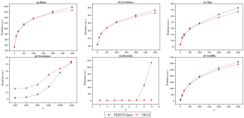
The efficiency of the algorithm is measured by its execution time considering not only the running time used by the CPU but also the access time required for disk input/output. The execution times of the TKHUS-Span algorithm compared to the proposed TKUS under different on the six datasets are shown in Figure 5. From the experimental results, it can be seen that the TKUS algorithm performs better overall for all datasets. In particular, with increasing on the Kosarak dataset, the execution time of TKHUS-Span dramatically increases when becomes greater than 12, whereas that of TKUS remains relatively stable. This is expected as the proposed strategies help to improve the efficiency of TKUS. However, the two algorithms take negligible time to finish top- HUSPM with a comparatively small value of . Moreover, TKUS has bad performance on the Yoochoose dataset, and we speculate that the massive calculations of 1- and 2-sequences ahead of the mining incurred very high computational costs. On the other four datasets, the execution time increases with increasing , where the growth curve clearly resembles a logarithmic function. The difference is that TKHUS-Span requires more running time with the same value of , and the gap grows with increasing . This demonstrates that the developed projection and local search mechanism and several strategies play a key role in improving the performance.
5.5 Memory Evaluation
Moreover, TKUS outperforms TKHUS-Span generally in terms of memory usage. The results for the memory usage are illustrated in Figure 6. It can clearly be seen that TKUS has better performance than TKHUS-Span in terms of memory usage in most cases. As can be seen from the results on Kosarak and Syn80k, the memory consumed by TKUS is less than that by TKHUS-Span in all instances because the proposed TKUS is able to avoid handling a large number of candidates in the mining process. In addition, there are few cases in the first four datasets where TKUS utilizes more memory, which is probably because TKUS requires more storage space to save the utility and PEU values of all 1- and 2-sequences with the SUR strategy. In general, the memory consumed becomes larger with increasing . However, there are some exceptions. Consider the example in Figure 6; the memory usage on the Yoochoose dataset is only slightly less than before when setting = 10000. As another example, on the dataset Sign, the memory consumption sharply decreases as passes 1000. On the whole, TKUS adopts efficient strategies to significantly improve performance in terms of memory usage. Nonetheless, TKUS still has much room for improvement in terms of memory consumption, especially for large .

5.6 Scalability
We conducted experiments to evaluate the scalability of TKUS on a synthetic database. We increased its data size through duplication with the purpose of obtaining a series of datasets with different sizes varying from 10K to 120K. The experimental results in terms of execution time and memory with set to 500 are shown in Figure 7. It is clear that TKHUS-Span has a worse performance than TKUS on the two metrics. As can be seen, the execution time increases linearly as the number of -sequences contained in the databases grows. On the dataset with 120K size, the execution times of the two algorithms are less than those on the dataset with 80K -sequences. In terms of memory usage, there is also a slight decrease when the algorithm addresses the dataset with 120K size because its unique distribution of utility values leads the SUR strategy to increase the minimum utility threshold significantly. From Figure 7, we can conclude that the TKUS algorithm is scalable to large-scale datasets because the running time and memory consumption are almost linearly related to dataset size.

6 Conclusions
In this paper, we first defined some key notations and concepts of SPM and formulated the problem of top- HUSPM. To handle top- HUSPM efficiently, we then proposed a novel algorithm called TKUS. For further efficiency improvement, TKUS adopts a projection and local search mechanism and follows several strategies, including SUR, TDE, and EUI, which are able to greatly reduce the search space and speed up the mining process. Finally, we conducted substantial experiments on six datasets with varied characteristics. The experimental results show that TKUS has good performance in terms of execution time, number of candidates, scalability, and more. We can conclude that TKUS is able to increase the minimum utility threshold quickly and extract the top- HUSPs efficiently. Our future work will apply the proposed TKUS algorithm to big data. For example, several extensions of the TKUS algorithm can be considered, such as adopting parallel techniques, such as Hadoop, to increase its speed.
Acknowledgment
Thanks for the anonymous reviewers for their insightful comments, which improved the quality of this paper. This research was partially supported by the National Natural Science Foundation of China (Grant No. 62002136), Natural Science Foundation of Guangdong Province, China (Grant No. 2020A1515010970), and Shenzhen Research Council (Grant No. GJHZ20180928155209705)
References
References
- [1] Rakesh Agrawal and Ramakrishnan Srikant. Mining sequential patterns. In Proceedings of the 11-th International Conference on Data Engineering, pages 3–14. IEEE, 1995.
- [2] Rakesh Agrawal, Ramakrishnan Srikant, et al. Fast algorithms for mining association rules. In Proceedings of the 20th International Conference on Very Large Data Bases, volume 1215, pages 487–499, 1994.
- [3] Chowdhury Farhan Ahmed, Syed Khairuzzaman Tanbeer, and Byeong-Soo Jeong. Mining high utility web access sequences in dynamic web log data. In 11th ACIS International Conference on Software Engineering, Artificial Intelligence, Networking and Parallel/Distributed Computing, pages 76–81. IEEE, 2010.
- [4] Chowdhury Farhan Ahmed, Syed Khairuzzaman Tanbeer, and Byeong-Soo Jeong. A novel approach for mining high-utility sequential patterns in sequence databases. ETRI journal, 32(5):676–686, 2010.
- [5] Oznur Kirmemis Alkan and Pinar Karagoz. CRoM and HuspExt: Improving efficiency of high utility sequential pattern extraction. IEEE Transactions on Knowledge and Data Engineering, 27(10):2645–2657, 2015.
- [6] Jay Ayres, Jason Flannick, Johannes Gehrke, and Tomi Yiu. Sequential pattern mining using a bitmap representation. In Proceedings of the 8th ACM SIGKDD International Conference on Knowledge Discovery and Data Mining, pages 429–435, 2002.
- [7] Jinlin Chen. An updown directed acyclic graph approach for sequential pattern mining. IEEE Transactions on Knowledge and Data Engineering, 22(7):913–928, 2009.
- [8] Ding-Ying Chiu, Yi-Hung Wu, and Arbee LP Chen. An efficient algorithm for mining frequent sequences by a new strategy without support counting. In Proceedings of the 20th International Conference on Data Engineering, pages 375–386. IEEE, 2004.
- [9] Thu-Lan Dam, Kenli Li, Philippe Fournier-Viger, and Quang-Huy Duong. An efficient algorithm for mining top-k on-shelf high utility itemsets. Knowledge and Information Systems, 52(3):621–655, 2017.
- [10] Tai Dinh, Van-Nam Huynh, and Bac Le. Mining periodic high utility sequential patterns. In Asian Conference on Intelligent Information and Database Systems, pages 545–555. Springer, 2017.
- [11] Quang-Huy Duong, Bo Liao, Philippe Fournier-Viger, and Thu-Lan Dam. An efficient algorithm for mining the top-k high utility itemsets, using novel threshold raising and pruning strategies. Knowledge-Based Systems, 104:106–122, 2016.
- [12] CI Ezeife, Yi Lu, and Yi Liu. PLWAP sequential mining: open source code. In Proceedings of the 1st International Workshop on Open Source Data Mining: Frequent Pattern Mining Implementations, pages 26–35, 2005.
- [13] Usama Fayyad, Gregory Piatetsky-Shapiro, and Padhraic Smyth. From data mining to knowledge discovery in databases. AI magazine, 17(3):37–37, 1996.
- [14] Philippe Fournier-Viger, Ted Gueniche, and Vincent S Tseng. Using partially-ordered sequential rules to generate more accurate sequence prediction. In International Conference on Advanced Data Mining and Applications, pages 431–442. Springer, 2012.
- [15] Philippe Fournier-Viger, Jerry Chun-Wei Lin, Rage Uday Kiran, Yun Sing Koh, and Rincy Thomas. A survey of sequential pattern mining. Data Science and Pattern Recognition, 1(1):54–77, 2017.
- [16] William J Frawley, Gregory Piatetsky-Shapiro, and Christopher J Matheus. Knowledge discovery in databases: An overview. AI magazine, 13(3):57–57, 1992.
- [17] Wensheng Gan, Chun-Wei Lin, Philippe Fournier-Viger, Han-Chieh Chao, Vincent Tseng, and Philip S Yu. A survey of utility-oriented pattern mining. IEEE Transactions on Knowledge and Data Engineering, page DOI: 10.1109/TKDE.2019.2942594, 2019.
- [18] Wensheng Gan, Jerry Chun-Wei Lin, Philippe Fournier-Viger, Han-Chieh Chao, Tzung-Pei Hong, and Hamido Fujita. A survey of incremental high-utility itemset mining. Wiley Interdisciplinary Reviews: Data Mining and Knowledge Discovery, 8(2):e1242, 2018.
- [19] Wensheng Gan, Jerry Chun-Wei Lin, Philippe Fournier-Viger, Han-Chieh Chao, and Philip S Yu. A survey of parallel sequential pattern mining. ACM Transactions on Knowledge Discovery from Data, 13(3):1–34, 2019.
- [20] Wensheng Gan, Jerry Chun-Wei Lin, Jiexiong Zhang, Han-Chieh Chao, Hamido Fujita, and Philip S Yu. ProUM: Projection-based utility mining on sequence data. Information Sciences, 513:222–240, 2020.
- [21] Wensheng Gan, Jerry Chun-Wei Lin, Jiexiong Zhang, Philippe Fournier-Viger, Han-Chieh Chao, and Philip S Yu. Fast utility mining on sequence data. IEEE Transactions on Cybernetics, 2020.
- [22] Jiawei Han, Jian Pei, Behzad Mortazavi-Asl, Qiming Chen, Umeshwar Dayal, and Mei-Chun Hsu. FreeSpan: frequent pattern-projected sequential pattern mining. In Proceedings of the 6-th ACM SIGKDD International Conference on Knowledge Discovery and Data Mining, pages 355–359, 2000.
- [23] Jiawei Han, Jian Pei, Behzad Mortazavi-Asl, Helen Pinto, Qiming Chen, Umeshwar Dayal, and Meichun Hsu. PrefixSpan: Mining sequential patterns efficiently by prefix-projected pattern growth. In Proceedings of the 17th International Conference on Data Engineering, pages 215–224. IEEE Washington, DC, USA, 2001.
- [24] Yen-Hui Liang and Shiow-Yang Wu. Sequence-Growth: A scalable and effective frequent itemset mining algorithm for big data based on mapreduce framework. In IEEE International Congress on Big Data, pages 393–400. IEEE, 2015.
- [25] Jian Pei, Jiawei Han, Behzad Mortazavi-Asl, and Hua Zhu. Mining access patterns efficiently from web logs. In Pacific-Asia Conference on Knowledge Discovery and Data Mining, pages 396–407. Springer, 2000.
- [26] Heungmo Ryang and Unil Yun. Top-k high utility pattern mining with effective threshold raising strategies. Knowledge-Based Systems, 76:109–126, 2015.
- [27] Bai-En Shie, Hui-Fang Hsiao, Vincent S Tseng, and Philip S Yu. Mining high utility mobile sequential patterns in mobile commerce environments. In Proceeding of the International Conference on Database Systems for Advanced Applications, pages 224–238. Springer, 2011.
- [28] Ramakrishnan Srikant and Rakesh Agrawal. Mining sequential patterns: Generalizations and performance improvements. In Proceeding of the International Conference on Extending Database Technology, pages 1–17. Springer, 1996.
- [29] Tin Truong-Chi and Philippe Fournier-Viger. A survey of high utility sequential pattern mining. In High-Utility Pattern Mining, pages 97–129. Springer, 2019.
- [30] Vincent S Tseng, Cheng-Wei Wu, Philippe Fournier-Viger, and S Yu Philip. Efficient algorithms for mining top-k high utility itemsets. IEEE Transactions on Knowledge and data engineering, 28(1):54–67, 2015.
- [31] Petre Tzvetkov, Xifeng Yan, and Jiawei Han. TSP: Mining top- closed sequential patterns. Knowledge and Information Systems, 7(4):438–457, 2005.
- [32] Jianyong Wang, Jiawei Han, and Chun Li. Frequent closed sequence mining without candidate maintenance. IEEE Transactions on Knowledge and Data Engineering, 19(8):1042–1056, 2007.
- [33] Jianyong Wang, Jiawei Han, Ying Lu, and Petre Tzvetkov. TFP: An efficient algorithm for mining top- frequent closed itemsets. IEEE Transactions on Knowledge and Data Engineering, 17(5):652–663, 2005.
- [34] Jun-Zhe Wang, Jiun-Long Huang, and Yi-Cheng Chen. On efficiently mining high utility sequential patterns. Knowledge and Information Systems, 49(2):597–627, 2016.
- [35] Cheng Wei Wu, Bai-En Shie, Vincent S Tseng, and Philip S Yu. Mining top- high utility itemsets. In Proceedings of the 18th ACM SIGKDD International Conference on Knowledge Discovery and Data Mining, pages 78–86, 2012.
- [36] Zhenglu Yang, Yitong Wang, and Masaru Kitsuregawa. LAPIN: effective sequential pattern mining algorithms by last position induction for dense databases. In International Conference on Database Systems for Advanced Applications, pages 1020–1023. Springer, 2007.
- [37] Hong Yao, Howard J Hamilton, and Cory J Butz. A foundational approach to mining itemset utilities from databases. In Proceedings of the 2004 SIAM International Conference on Data Mining, pages 482–486. SIAM, 2004.
- [38] Junfu Yin, Zhigang Zheng, and Longbing Cao. USpan: an efficient algorithm for mining high utility sequential patterns. In Proceedings of the 18th ACM SIGKDD International Conference on Knowledge Discovery and Data Mining, pages 660–668, 2012.
- [39] Junfu Yin, Zhigang Zheng, Longbing Cao, Yin Song, and Wei Wei. Efficiently mining top- high utility sequential patterns. In IEEE 13th International Conference on Data Mining, pages 1259–1264. IEEE, 2013.
- [40] Mohammed J Zaki. SPADE: An efficient algorithm for mining frequent sequences. Machine Learning, 42(1-2):31–60, 2001.
- [41] Chuankai Zhang, Yiwen Zu, Junli Nie, and Linzi Du. Two efficient algorithms for mining high utility sequential patterns. In IEEE Intl Conf on Parallel & Distributed Processing with Applications, Big Data & Cloud Computing, Sustainable Computing & Communications, Social Computing & Networking, pages 905–911. IEEE, 2019.
- [42] Chunkai Zhang, Zilin Du, and Yiwen Zu. An efficient algorithm for extracting high-utility hierarchical sequential patterns. Wireless Communications and Mobile Computing, 2020, 2020.
- [43] Chunkai Zhang and Yiwen Zu. An efficient parallel high utility sequential pattern mining algorithm. In IEEE 21st International Conference on High Performance Computing and Communications; IEEE 17th International Conference on Smart City; IEEE 5th International Conference on Data Science and Systems, pages 2798–2803. IEEE, 2019.
- [44] Chunkai Zhang, Yiwen Zu, Junli Nie, Linzi Du, Jingqi Du, Siyuan Hong, and Wenping Wu. A fast algorithm for hiding high utility sequential patterns. In IEEE Intl Conf on Parallel & Distributed Processing with Applications, Big Data & Cloud Computing, Sustainable Computing & Communications, Social Computing & Networking, pages 1316–1322. IEEE, 2019.
- [45] Morteza Zihayat and Aijun An. Mining top-k high utility patterns over data streams. Information Sciences, 285:138–161, 2014.
- [46] Morteza Zihayat, Heidar Davoudi, and Aijun An. Top- utility-based gene regulation sequential pattern discovery. In IEEE International Conference on Bioinformatics and Biomedicine, pages 266–273. IEEE, 2016.