Analytical representation for amplitudes and differential cross section of pp elastic scattering at 13 TeV
Abstract
With analytical representation for the pp scattering amplitudes introduced and tested at lower energies, a description of high precision is given of the data at = 13 TeV for all values of the momentum transfer, with explicit identification of the real and imaginary parts. In both and coordinates the amplitudes have terms identified as of non-perturbative and perturbative nature, with distinction of their influences in forward and large ranges and in central and peripheral regions respectively. In the forward range, the role of the Coulomb-nuclear interference phase is investigated. The energy dependence of the parameters of the amplitudes are reviewed and updated, revealing a possible emergence of a peculiar behavior of elastic and inelastic profiles in b-space for central collisions, which seems to be enhanced quickly at higher energies. Some other models are also briefly discussed in comparison, including the above mentioned behavior in b-space.
Keywords:
pp elastic scattering; hadronic amplitudesI Introduction
Totem Collaboration in LHC has produced two sets of data data on elastic pp scattering at =13 TeV in separate publications Totem_13_1; Totem_13_2; Totem_13_3, covering the following ranges
- •
Set I - , with N=138 points Totem_13_1 ;
- •
Set II - , with N=290 points Totem_13_2 .
With respect to systematic errors, the two sets of measurement are presented with very different features: errors of about 5 for I and less than 1 (except for the first 11 points) for Set II. The situation, illustrated in Fig.1, influences the analysis of the data. The very large systematic errors in Set I indicates the necessity of special care on its use for the determination of the forward scattering structure.
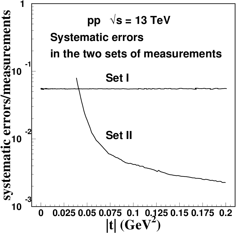
There are 56 points of small in Set I, up to , where Set II starts, and thus there is a basis of 56 + 290 = 346 data points to perform a global description of the 13 TeV data. We also build a combined file merging the points of the common range, with a total of 138+290=428 points that are used in an overall test.
The data of Set I have been studied PLB2019 with forms of amplitudes restricted to small values. The treatment of this range requires detailed account of the Coulomb-nuclear interference, and it was shown that the model-independent determination of the amplitude in these representations is unreliable with the present data alone, due to the small value of the parameter and to the assumption of a model for the treatment of the Coulomb-nuclear interference phase that needs to be tested at such high energies. In the forward direction the real part contributes to only about 1% of the observed , and it is necessary to have a well-inspired extraction of the imaginary part, requiring data of very regular behaviour, to allow the determination of the properties of the real part, such as the parameter and the amplitude slope.
Putting all information together, we achieve a unified treatment of 428 data points, identifying analytically the real and imaginary parts (with 4 parameters each) of the complex elastic amplitude, with remarkable values with statistical and systematic errors added in quadrature and calculated with statistical errors only. Everywhere in the present text is a short for . The graphical representation of this result is shown in Fig.2. The present treatment is similar to previous work that was very effective at lower energies 1.8 - 1.96 TeV of Fermilab KFK_1 and 7-8 TeV of LHC KFK_2; KFK_3.
The large range of Set II is coupled sensibly with the (energy independent) tail of perturbative three-gluon exchange observed at Faissler, with 39 points in the range . The first identification of the energy independence of the behaviour for large in pp elastic scattering was made in the comparison of data at = 19.6 and 27.4 GeV Conetti. The theoretical explanation for the behaviour of for large in terms of the real three-gluon exchange amplitude was given by Donnachie and Landshoff DL1. The universality is demonstrated for energies below = 62.5 GeV in Fermilab and CERN/ISR measurements flavio1; flavio2 (see figures in these two papers), showing smooth connection between the range of small and mid- combining perturbative and nonperturbative terms and the range of large of FNAL Faissler measurements dominated by three-gluon exchange. The role of the real amplitude in the large sector of pp elastic scattering is then confirmed.
The transition range from 2 to 5 gives information on the magnitude and sign of the real part of the hadronic amplitude, that is dominant for large . Unfortunately the LHC pp measurements at 7 and 8 TeV KFK_2; KFK_3 are restricted to less than , and the connection between mid and large regions remained in the non-quantitative level, although there is clear indication , as shown in Fig.6 of the 7 TeV paper KFK_2, where the data at 52.8 GeV and 7 TeV are exhibited. At 13 TeV the measurements reach almost , allowing investigation in an important extended range. Using the same representation described above, with a proper connection between the 13 TeV and the 17.4 GeV data, we obtain an analytical form embracing 467 (= 428+39) data points, with and using total errors (combined statistical and systematic) and pure statistical errors respectively.
The present work uses the amplitudes introduced in previous papers KFK_1; KFK_2; KFK_3, expressed in both and coordinates, with explicit forms for the real and imaginary amplitudes: the disentanglement of the two parts is essential for the description of the dynamics of the process. The superposition of non-perturbative and perturbative terms in both real and imaginary parts produces remarkable structure in the elastic differential cross section that faithfully reproduces the data. In the following this framework is referred to as KFK model.

In Sec.II we review the construction of the amplitudes in the KFK model, inspired on the early applications of the Stochastic Vacuum Model (SVM) to high-energy elastic scattering. The and space coordinates are analytically related, with terms representing perturbative and non-perturbative dynamics.
In Sec.III we apply the KFK amplitudes to describe in detail the forward, mid and large ranges, obtaining a unique solution valid with high precision for all , as shown in Fig.2. Separate attention is given to an extension of the representation to the range of high measured at 27.4 GeV Faissler and also to the small range of Set I re-examining the role of the Coulomb-nuclear interference phase PLB2019. In Sec.IV, the properties of the amplitudes in - and - coordinates are described and discussed in separate subsections. In Sec.V we insert the results of the present analysis at 13 TeV in the previous study of energy dependence of the KFK framework, updating description and predictions. There, we report a new behaviour of the profile functions in b-space in the domain of central collisions, which seems to be enhanced quickly at high energies. This observation was not possible without the present 13 TeV data. Sec.VI compares our description with other models and Sec.VII presents remarks and critical evaluation.
II KFK model : Analytical Representation of the amplitudes
The Stochastic Vacuum Model(SVM) is based on the functional integral approach Nachtmann1 to high energy scattering that relates high energy scattering with nontrivial properties of QCD vacuum Dosch; Dosch_Simonov. The central element is the gauge invariant Wegner-Wilson loop, and physical quantities are obtained from the vacuum expectation values of the correlations of two loops, defined in terms of coordinates in the transverse collision plane. Assuming dominance of Gaussian fluctuations in the field strengths, the calculation becomes fully analytical. Observables are written in terms of physical quantities: the value of the gluon condensate,that determines the strength of this non-perturbative dynamics, and the correlation length, that is the parameter of the loop-loop correlation function that sets the scale for the geometric dependence in -space. These quantities have values fixed by hadronic properties and by lattice calculations DiGiacomo; Meggiolaro. With analytic continuation from Euclidean to Minkowski space SVM3 gauge-invariant dipole-dipole scattering is constructed.
The amplitude of non-perturbative hadron-hadron scattering in the eikonal approximation is factorized with the product of the correlation of loops (representing elastic scattering of two colour dipoles) and the factor with the dipole contents in the light-cone wave functions of the colliding hadrons SVM; SVM1; SVM2. The overlap of the loop-loop correlation with the hadronic wave-functions of finite size leads to structure of profile function where the basic correlation parameter becomes spread, appearing with effective value that depends on the hadronic sizes and, in case of scattering amplitudes, can also be modified by the collision energy. These effective representations of the correlations proper of the QCD vacuum are not expected to be very different from the static lattice determination.
Besides hadron-hadron scattering, the concept of the loop-loop correlation was also applied to the non-perturbative exclusive photo- and electroproduction of vector mesons SVM2; Photo; Electro.
The KFK model writes analytical forms for the pp and elastic scattering amplitudes in and spaces, based on previous experience with the Stochastic Vacuum Model (SVM) SVM, using a scale (correlation) length parameter and the asymptotic (large ) behaviour of the profile function as guiding ingredients.
KFK model introduced non-perturbative and perturbative contributions flavio1; flavio2, later assumed as necessary long and short range terms in the loop-loop correlation SVM2. The effective gluon mass introduced to control the infrared range in the perturbative correlator enters in the overlap product with the proton dipole content and appears in the profile function in KFK through a simple Gaussian term as in Eq.(1).
The T-matrix element in SVM is purely imaginary, and with missing real part cannot be calculated in the full range. KFK introduces a real part that is a mirror image of the imaginary amplitude. The real part is dominant for large , and has crucial role in the dip-bump region of pp elastic scattering around 0.4-0.5 where the imaginary part passes through zero. The sophisticated dip-bump structure in requires delicate property of the real part valid in this range. Both parts must have perturbative and non-perturbative terms, and must have zeros, signs and magnitudes following theoretical principles and reproducing observations flavio1; flavio2. The zero in the real part at small predicted by a theorem by A. Martin Martin, is confirmed with the LHC data MURILO. while the imaginary part has a zero responsible for the dip-bump structure in .
The analytical forms proposed for the non-perturbative terms of the amplitudes are inspired in the behaviour of the profile function for large found in the calculation with SVM flavio1; SVM, with a combined exponential-Yukawa dependence. The Fourier transforms to -space present features that can effectively represent the data for all . As is not an observable quantity, the construction is tested in space, and parameters are fixed by experiments. Accurate description of the data is obtained with four parameters in each part of the complex amplitude.
The disentanglement of the two parts of the complex amplitude is not at all trivial. The connection with the three-gluon exchange contribution helps in the identification of the sign and magnitude of the real part, and an additional term for perturbative three-gluon exchange is introduced separately.
The KFK model has been investigated at several energies, and the energy dependence of the parameters comes out smooth, with simple parametrization KFK_1; KFK_2; KFK_3.
II.1 Impact parameter representation
The amplitudes in the Stochastic Vacuum Model SVM are originally constructed through -space profile functions, that give insight for geometric aspects of the collision, playing role in the eikonal representation, where unitarity constraints have interesting formulation. The dimensionless amplitudes of the pure nuclear interaction are written in the form
| (1) |
with a Gaussian term meant to be of perturbative nature and a characteristic non-perturbative shape function
| (2) |
The label indicates either the real or the imaginary part of the complex amplitude.
The quantity , called correlation length, represents properties of the QCD vacuum, where it sets the scale for the loop-loop correlation, with determination in static (Euclidean space) lattice calculation DiGiacomo as 0.25-0.30 fm. After analytic continuation to Minkowski space and overlap with the hadronic wave functions, the non-perturbative scale appears in profile functions of hadron-hadron scattering, with effective value modified inside this range. In the present work for pp scatering at 13 TeV we find the value
| (3) |
The parameters with units in and dimensionless are functions of the energy. They are determined for TeV with high precision in Sec.III, leading to explicit analytical expressions for the imaginary and real amplitudes. The Gaussian form of the first term in Eq.(1) corresponds to the perturbative part of the loop-loop correlation introduced in developments of SVM, following results suggested by lattice calculations. The second term, referred to as shape function, corresponds to contributions from non-perturbative loop-loop correlation function. It is zero at , , and is normalized as
| (4) |
Eq.(1) represents a parametrized formulation of the profile function based on the SVM proposal. The perturbative and non-perturbative terms of the amplitudes are dominant for small and large respectively. For large , corresponding to peripheral collisions, the amplitudes fall down with a exponential-Yukawa-like tail,
| (5) |
that reflects the correlations of loops at large distances. This asymptotic behaviour inspired the construction of the shape function for Eq.(1).
II.2 -space representation
In the classical limit the variable is connected with the impact parameter, but it is not directly observable, and the treatment of data is made in space. One advantage of the shape function in KFK is that there is explicit analytic Fourier transformation for the amplitudes in Eqs.(1,2), so that the scattering properties can be studied directly in both frameworks.
In our normalization the elastic differential cross section is written
| (6) | |||||
with and in units, and
The complete amplitudes , contain the nuclear and the Coulomb parts as
| (7) |
and
| (8) |
where is the fine-structure constant, is the interference phase (CNI) and is related with the proton form factor
| (9) |
for the ppp collisions. The proton form factor is taken as
| (10) |
where GeV2.
We recall the new measurements of the proton radius proton_radius and changes in the proton form factor proton_formfactor. These changes in the electromagnetic and hadronic structure of the proton may become important for the analysis of forward elastic scattering, when their quality improves. As it has been proved PLB2019, this is not the case at the present, and we use the quantities as written above.
The expressions and represent the nuclear amplitudes for the terms written in Eq.(1). The non-perturbative shape functions in -space obtained by Fourier transforms are written
| (11) | |||||
with the property
| (12) |
Use is made of the integration formula
| (13) |
In addition to the Fourier transform of the perturbative part in Eq.(1) we introduce in the real part a term representing the perturbative three-gluon exchange DL1; flavio1 that appears in the large region, and the complete nuclear amplitudes are then written
| (14) | |||
with , and where the Kronecker delta symbol is introduced so that contributes only to the real part. Eqs.(11,14) constitute the KFK model for the pp and elastic amplitudes in space.
The limits of the amplitudes for small give the total cross section (optical theorem), the ratio of the real to imaginary amplitudes and the slopes at through
| (15) | |||||
| (16) |
and
| (17) | |||||
The tail term , producing a universal (not energy dependent) form for large in was studied in the analysis of the experiments at CERN-ISR, CERN-SPS flavio1, 1.8 TeV KFK_3 and 7 TeV KFK_1. To restrict this contribution to the large region, we create a connection factor, writing
| (18) |
where the last two factors cut-off this term smoothly in the domain from 2 to 5.5 , and the signs refer to the pp and p amplitudes respectively. The detailed form of the factor in Eq.(18) must be adequate for the description of the data for values in the transition range connecting the experimental points Faissler at . In Sec.III, the proposed parameters are
| (19) | |||
The peculiar form of Eq.(18) is explained in Subsection III.1.
III Description of the 13 data
In this section we obtain the representation of the data of Totem experiment at 13 TeV through the -space amplitudes of the KFK model written in Eqs.(11,14,18). Plots in Fig.3 show separately forward, mid and full ranges of the data of Sets I and II, described by a unique solution, with the parameters given in Table 1. Table 2 gives statistical quantities for different ranges of the data, obtained with the same unique solution. Values of are given for calculations with statistical errors and for total errors combining statistical and systematic errors in quadrature. We also inform the value for a combined set of the first 56 points of Set I with the 290 points of Set II (total 346 points), avoiding the superposition of ranges. In the last line of Table 2 we inform the result for a set of 467 points joining the 27.4 GeV data Faissler, using the real amplitude that includes the term of 3-gluon exchange as in Eqs.(14, 18), while keeping fixed the parameters of Table 1. The connection of the data of these different energies is illustrated in Subsec.III.1. In Subsec.III.2 we present specific results of an analysis for the forward data of Set I.
Observable quantities and positions of the zeros are given in Table 3.


| Imaginary Amplitude | Real Amplitude | ||||||
|---|---|---|---|---|---|---|---|
| N | range | (total) | (total) | (stat) | (stat) | Remarks |
|---|---|---|---|---|---|---|
| pts | no tail | with tail | no tail | with tail | ||
| 138 | 0.000879-0.201041 | 0.0162 | — | 1.455 | entire Set I | |
| 260 | 0.000879-0.24902 | 0.2737 | — | 4.852 | Set I(138) + Forward Set II (122) | |
| 122 | 0.0384-0.24902 | 0.5866 | — | 9.066 | Forward part of Set II | |
| 144 | 0.25643-0.89633 | 3.068 | — | 5.643 | dip-bump region in Set II | |
| 152 | 0.25643-1.15991 | 3.187 | — | 5.690 | extended dip-bump region in Set II | |
| 24 | 0.91528-3.82873 | 10.74 | 12.72 | 11.73 | 13.70 | range of highest in Set II |
| 290 | 0.0384-3.82873 | 2.326 | 2.448 | 7.052 | 7.164 | entire Set II |
| 346 | 0.000879-3.82873 | 1.943 | 2.044 | 6.142 | 6.235 | Set I(56) + Set II(290) |
| 428 | 0.000879-3.82873 | 1.567 | 1.642 | 5.186 | 5.260 | Set I(138) + Set II(290) |
| 385 | 0.000879-14.2 | — | 2.103 | — | 5.869 | Set I(56) + Set II(290) + Faissler et al (39) |
| 467 | 0.000879-14.2 | — | 1.731 | — | 5.042 | Set I(138) + Set II(290) + Faissler et al (39) |
| Imaginary Amplitude | Real Amplitude | Elast. | Inel. | Dip | ||||||
|---|---|---|---|---|---|---|---|---|---|---|
| mb | mb | mb | mb/ | |||||||
| 0.47 | 0.025 | |||||||||
III.1 Connection with measurements at
The elastic scattering data for larger than 5 have been shown to be independent of the energy in a large range of from 20 GeV to 7 TeV Faissler; Conetti; flavio1; KFK_1. The experiment at with 39 data points covering the wide range from 5.5 to 14.2 Faissler, provides important reference for the study of pp at large scattering angles. The property is demonstrated for energies below = 62.5 GeV in Fermilab and CERN/ISR measurements flavio1 (see Figures 2,3 and 10 in this paper), showing a smooth connection between the mid- range containing perturbative and nonperturbative terms and the range of large dominated by perturbative three-gluon exchange.
The universality in the energy and the dependence of form in have been interpreted by Donnachie and Landshoff DL1 as determined by the process of exchange of three gluons. This contribution is represented by the quantity introduced in Eq.(14), receiving a cut-off factor written in Eq.(18) designed to restrict the behaviour. The three-gluon contribution occurs in the range where the imaginary part is negligible, and the perturbative term is dominant. The transition from 2 to 5 is precious to inform features (signs, magnitudes) of terms of the real scattering amplitude in the large region. These features are described in Sec.IV.
As an example, the structure of the real amplitude leads to the argument that the difference in the dip regions of pp and scattering at 53 GeV Breakstone is due to the difference in the signs of the three-gluon contributions in pp and scattering, and not necessarily to the presence of an odderon element flavio1, unless it is meant that three-gluon exchange is the modern QCD name for odderon Ewerz; Levin.
At high energies, there is not sufficient experimental information for the investigation of the elastic amplitudes at high . LHC measurements at 7 and 8 TeV KFK_2; KFK_3 are restricted to less than , and the connection between mid and large regions remains in the level of clear indication, as shown in Fig.6 of the 7 TeV paper KFK_2, where the data for 52.8 GeV Nagy; Amos and 7 TeV are exhibited together.
At 13 TeV the data are more extended in , reaching nearly 4 , allowing investigation of properties of the amplitudes in the connection with FNAL data Faissler. Then we first choose the parameters for the function, that is shown Fig.4, together with the corresponding cross section in the range of the transition. In Fig.5 we show the matching of the Totem 13 TeV and ISR 52.806 GeV measurements Nagy; Amos with the data of FNAL measurements Faissler at .


Some points of high of the Totem measurements show a marked decrease in the values of , with large statistical error bars, from 45% to 60%. These points deviate meaningfully from the proposed solution, and particularly they seem not to accept easily the suggestion of connectivity with the three-gluon tail. These are only few points of poor statistics, but visually they have important influence, as shown in Figs.4 and 5. In our description, this range of is dominated by the perturbative term in the real amplitude, and serves as important test of the proposed disentanglement. In Sec.IV we show that the real part of the KFK amplitude is positive for large , and then the superposition with the also positive three-gluon term should be constructive. If the real part were negative, a dip could be formed. In the analysis of the 1.8/1.96 GeV Fermilab KFK_1 data we predicted that such dip would appear for large (the three gluon term is negative in ), but unfortunately the measurements do not reach large enough , and the prediction is not tested. Here in pp at 13 TeV, we do not have simple explanation for the decrease of in the points of largest . A connection function producing the visual shape would not be natural. This question obviously leads to the suggestion that the measurements in the large range should receive more attention.
Table 2 shows that the 24 points of with highest in Set II are described in our unique solution with comparatively large values of about 10. This is a local feature, as these points have low influence in the value for the 428 points. For a local investigation, we observe that this range is dominated by the perturbative real part, so that only the parameters and require attention. Thus, with and we obtain and , respectively using total and only statistical errors. This predicted local improvement in changing only two selected parameters is consequence of the separation of the perturbative and non-perturbative terms in the analytical form.
III.2 Specific representation of amplitudes for the 138 points of Set I
As a side information (since the main concern of the present work is with the unique global solution for all ranges), in Table 4 we show the results for the 138 points of Set I with freedom given to the and parameters, maintaining all other quantities as written and used in Tables 1 and 2. Only the non-perturbative magnitudes and are investigated in this alternative examination because these terms are dominant in the imaginary and real amplitudes for small , as shown in Sec.IV. Comparison is made of solutions with and without inclusion of the Coulomb-nuclear interference phase . The results in Table 4 may be compared with values obtained with simplified forms of amplitudes restricted to the forward scattering range PLB2019, namely with product of exponential and linear factors as
| (20) |
We again stress that the parameters , and slopes are model-dependent quantities, related to specific analytical forms of the amplitudes. The only experimental measurements are the values of at angular positions defined by values of . In particular, for the value of , it has been shown PLB2019 that the presently available data at small does not allow a conclusion about its value. Besides the insufficiency of regular data in the very forward region, the theoretical basis for the Coulomb-nuclear interference phase is uncertain.
We remark that both imaginary and real parts have zeros, so that, besides exponential slopes at least linear factors in the amplitudes are essential to represent the forward data realistically as in Eq.(20). In KFK the factorization of the logarithmic derivative with a slope as in Eq.(17) leaves a remainder that has a zero, but not a linear zero (actually the remaining factor has zero of higher order in a Taylor expansion), so that and in Eq.(17) correspond to the effective slope that includes the effect of a linear factor in the forward amplitude. The effective slope in Eq.(20) comparable to Eq.(17) is . It is also interesting to compare the value of the first real zero of the KFK model in Table 3 with the values obtained PLB2019 with Eq.(20). With , the zero at may be compared with in Table 3.
| CNI | ||||||||
|---|---|---|---|---|---|---|---|---|
| phase | mb | |||||||
| zero | 1.126 | 21.06 | 26.37 | 0.201 | ||||
| 1.121 | 21.08 | 25.96 | 0.213 |
IV Imaginary and real parts of the scattering amplitude
The analysis presented in Sec.III leads to a proposal for the disentanglement of the real and imaginary parts, that is obtained directly from the data. In this section we discuss the properties of the amplitudes and their terms, in both and coordinates.
IV.1 Amplitudes in space
Fig.6 shows the amplitudes, detailing small and large ranges. Similarly to lower energies, the imaginary and real parts have one and two zeros respectively. In the plot for large , the contribution of the the tail term is also shown, appearing as a deviation in the real amplitude visible for .
The separate perturbative and nonperturbative parts of the imaginary and real amplitudes are shown in Fig.7. The quantities. and are strong and with opposite signs in the dip-bump region, with a cancellation at , causing the dip. The existence of these two terms in is most important for the construction of the representation. The cancellation leaves room for the influence of the real amplitude that modulates the shape of the dip-bump structure. dominates (in magnitude) over in the dip-bump region, but if falls to zero more rapidly, while the perturbative real part lasts longer in . For larger than only the perturbative real part remains active, with positive sign.
As a general view, we observe that forward scattering emphasizes non-perturbative dynamics, while large scattering is dominated by perturbative terms in the real amplitude. The real part becomes negligible for , as decreases with the energy.
The magnitudes of all terms in the amplitudes vary enormously from the bump to the region = 3-4 reached by the present data. The structure in the large range that we try to access through the connection with the three-gluon exchange is important for the construction of a global picture for pp elastic scattering. This construction is confirmed by other models, as illustrated in Fig.(14).


IV.2 Amplitudes in -space
The -space dimensionless amplitudes and of Eqs.(1,2) are shown in Fig.8a,b, where we observe that there are no zeros. In general is about 10 times larger than , and it is impressive that the Fourier transforms of both have importance in the structure of the observed , with a dominance of the real part for large . The function is monotonically decreasing in , while has a maximum at with numerical value 0.131. At we have
that is slightly larger than and
At
we have
As seen in Fig.8, the non-perturbative terms , , dominate the amplitudes for large , while dominates over in the forward peak, where non-perturbative and perturbative magnitudes are in the ratio , with a ratio in the contributions to the total cross section. It is remarkable that forward elastic scattering is mainly a peripheral process of non-perturbative nature.
In terms of the amplitudes, the elastic, total and inelastic cross sections are written respectively
| (21) |
| (22) |
and
| (23) | |||||
The values of the integrated cross sections are mb, mb, mb, with ratio . The differential cross sections in -space shown in Fig.8c give a hint of the proton hadronic interaction structure in the transverse collision plane with smooth monotonous -dependence.
Unitarity imposes that . With a classical point of view, a hypothesis that the inequality is valid for all is written
| (24) |
or
| (25) |
This relation, called -space unitarity, is satisfied by our amplitudes.
The eikonal function for a given is introduced through
| (26) |
with
| (27) |
Separating real and imaginary parts
| (28) |
and
| (29) |
we obtain
| (30) |
so that the b-unitarity condition in Eq.(25) reads simply
| (31) |
With monotonic behavior of the scattering amplitudes, our solutions are restricted to the branch where . We need special care to write the expression for , because it enters the second quadrant for small . At the point where , becomes zero, and it is negative between and . To have continuity, avoiding that a calculator produces a positive value in the fourth quadrant, we must write the function with two arguments. In the form used by the Wolfram Mathematica software, we write
| (32) | |||||
In terms of the eikonal function, we have
| (33) | |||||
| (34) | |||||
| (35) |
These expressions are plotted in Fig.8, and the explicit representation for and the expression in Eq.(30) for are plotted in Fig.9.
The function is not monotonically decreasing, starting with , and presenting a maximum at with value . This property is not observed in our previous analyses at lower energies TeV, where is always monotonically decreasing function in . To detail this peculiar behaviour, and illustrate the effect of the real part, we point out that from Eqs. (28,29) together with Eq.(31) we have
| (36) |
The expression is plotted in dotted line in Fig.9a. At , where , touches . Everywhere else, the inequality holds. This happens even at the maximum of , where is slightly larger than =2.8818.
It is interesting that the differential inelastic cross section in Fig.8-c is almost fully saturated () in the central collision region up to fm. This can be seen also from the behavior of in Fig.9, where for , it is so that . In the classical picture, from the central to approximately the half overlap impact parameter, the pp system behaves as completely absorptive, leading to particle production channels. We note, however, that this does not mean that the elastic differential cross section is null, due to the wave nature of the scattering. The diffractive wave as the reflection of inelastic scattering contributes to the elastic channel with almost the same magnitude as the inelastic one inelastic one even for the extreme case of a black disk.
On the other hand, at this energy, we note that the elastic scattering profile at is rather large, exceeding the inelastic profile, which was never observed in our previous analyses. Furthermore, we also observe for the first time, a small decrease the inelastic profile near (almost invisible in Fig. 8, as direct reflection of the behavior of shown in Fig. 9). We will return to this point later.
As claimed in previous studies, in the very peripheral collisions (at this energy, ), contributions from elastic processes become negligible and inelastic processes are dominant.
Physically speaking, this part can be associated to diffractive particle production mechanism. In -space, this constitutes a rather diffused surface structure with a long tail in . We may associate such processes (forward scattering) with those from the excitation of the vacuum through the non-perturbative processes. In KFK_3 we argue that the existence of such a long tail in and vanishingly small values of for large , say , can be considered as responsible for the ratio, being significantly larger than that of a black-disk limit, namely . There, assuming the geometric scaling property for , we extrapolated this ratio to 13 TeV, predicting the value
while the present analysis gives
which is smaller, but yet definitely far from the black disk limit.


V Energy Dependence
The KFK model represented by Eqs.(1,2), or alternatively Eq. (14) in space, has been used in the description of data at several energies, and its properties and predictions in both and spaces were studied also for cosmic ray showers CR_2014.
Data of pp elastic scattering covering regularly from small to large are available in the ISR range (up to 63 GeV), and at 7 and 13 TeV in LHC Totem measurements. The comprehensive analysis of all data then available (up to =7 TeV) was made KFK_3 with a study of the energy dependence of the KFK parameters, including predictions for 13 and 14 TeV.
The 13 TeV data are more precise and cover wider range than the 7 TeV data, allowing realistic determination of the amplitudes in KFK model. This is the purpose and the achievement of the present work. The results obtained lead to revision and extension of the previous analysis, and the updated revision is presented in this section.
We stress that KFK provides a framework that is particularly important for a study of the real part, that is elusive in the forward region, becoming influent at mid and dominant after about 3 . Due to the small value of , the interplay of the electromagnetic and real part of the nuclear amplitude is very delicate. A detailed analysis of the forward data at 8 TeV TOTEM_8_TeV, accounting for the role of the real part of the hadronic amplitude in the CNI contribution, has demonstrated the importance of the hadronic model in the determination of the forward scattering parameters, leading to the values and . Particularly the value, small compared to 0.14 of COMPETE preference, anticipated the tendency that was later confirmed in measurements at 13 TeV. The value at 8 TeV affects the revision of parameters presented in this section, particularly leading to at 7 TeV, with very good . The decisive influence of the hadronic amplitudes in the study of the phase in the Coulomb-Nuclear Interference, with consequences in the evaluation of and , was also demonstrated at 13 TeV PLB2019.
Table 5 shows the optimal values of the model parameters for GeV, chosen as representative of the ISR range, together with the results of 7 TeV and 13 TeV. The table introduces an alternative notation, defining quantities through
| (37) |
that have the same units as the other six quantities , , , used instead of the dimensionless used in the text and in previous work.
| N | |||||||||||||
|---|---|---|---|---|---|---|---|---|---|---|---|---|---|
| TeV | mb | ||||||||||||
| 0.0528 | 1.39 | 97 | 0.9251 | 42.54 | 0.078 | 5.958 | 2.348 | 9.451 | 10.5778 | 0.0710 | 1.144 | 1.131 | 11.794 |
| 7 | 2.00 | 165 | 0.2957 | 98.75 | 0.115 | 13.730 | 4.100 | 22.040 | 16.3000 | 0.2572 | 1.405 | 3.856 | 15.576 |
| 13 | 2.1468 | 428 | 1.567 | 111.56 | 0.118 | 15.701 | 4.323 | 24.709 | 16.7858 | 0.2922 | 1.540 | 4.472 | 16.107 |
Using the forms instead of , the non-perturbative shape functions are written
| (38) |
Consequently, in -space the shape function obtained by Fourier Transform is written
| (39) | |||||
Using these sets of values, we updated the energy dependence of the KFK parameter values KFK_3 as
| (40) | |||
| (41) | |||
| (42) | |||
| (43) | |||
| (44) | |||
| (45) | |||
| (46) | |||
| (47) |
with in TeV and units for all quantities. These forms as functions of the energy are shown in Fig.10.
In the table we notice that the correlation length squared , serving as scale for the gluon correlations in the transverse collision plane for the nonperturbative term, has regular energy dependence, staying close to the value obtained in static lattice calculation. The KFK amplitudes for are sensitive to these values, and a representation appropriate for interpolation is
| (48) |

The slopes of the amplitudes, shown in Fig.11, can be represented by simple forms
| (50) | |||||
with units . The structure of the forward amplitude with different slopes and is crucial in the analysis of the CNI range for determination of and . The stronger real slope indicates the presence of the close zero predicted by Martin’s theorem.

It is interesting to observe the energy dependence of properties of the amplitudes in -space KFK_3; CR_2014. Fig.9 shows that at 13 TeV the elastic differential cross section at is larger than the inelastic quantity, while at lower energies the inverse is true. According to our description, the ratio elastic/inelastic at increases with the energy, with values 0.56, 0.90, 1.0, 1.06 for 52.8 GeV, 7 TeV, 10.57 TeV and 13 TeV respectively. The energy dependences are determined with data that have a wide coverage in t and permit to obtain the parameter values with excellent precision for each given energy up to 13 TeV. However, the forms have limited local validity, like Taylor expansions in up to second order, and are not adequate for extrapolation to very high energies. Nevertheless, it is tempting to compare the predictions resulting from the present analysis to, for example, a cosmic ray energy scale, as = 50 TeV.
The above mentioned ratio elastic/inelastic at increases as high as 1.56, while Eq.(49) predicts mb at 50 TeV, that is consistent with the estimated values of sigma(pA) data CR_2014. Values of some derived quantities are shown in Table 6.
Fig.12 shows the elastic, inelastic and total differential cross sections in -space for 13 and 50 TeV. In view of the study of properties of the terms of the amplitudes in subsection IV.2 we learn that this increase of the elastic cross section at is mainly due to the perturbative terms. However, we must remark that the range around is reduced in the integration, and that the inelastic cross section dominates for larger , so that the integrated inelastic is larger than the integrated elastic at all energies. The ratios are given in Table 6.
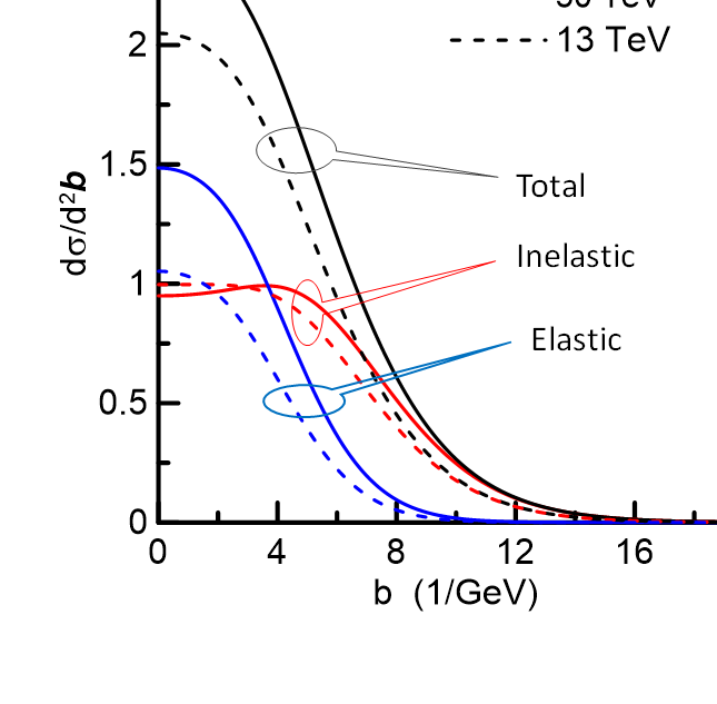
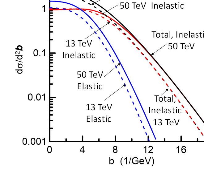
In Fig.12 we observe that the inelastic differential cross section is never saturated (namely it is always smaller than 1, with the eikonal larger than zero), while the elastic and total quantities are strongly enhanced in the region close to . For very central collisions, with the impact parameter smaller than the nucleon geometric size, inelastic processes at 50 TeV are visibly suppressed compared to the 13 TeV case. To be more precise, such suppressions of inelastic profile near already started in the 13 TeV data, although not being quite visible in the figure. However from the behavior of in Fig.9 near , together with Eq.(35), it is clear that the inelastic profile has a minimum at . as mentioned in the previous section. The ratio elastic/inelastic cross sections at increases fast because the elastic part increases and simultaneously the inelastic part decreases. For much higher energies, this tendency is more enhanced.
The concept of the impact parameter is classical and cannot be associated with a real physical observable in microscopic systems. Nevertheless, the present results suggest an image that, at ultra high energies, the two colliding protons tend to behave as two thin, inter-penetrable hard disks so that the process becomes elastic scattering dominant, decreasing the inelastic channel. This seems to occur in the -domain corresponding to the proton radius (). Such image may require the existence of some non-causal transverse correlation between the whole colliding protons, for example similar to the exclusion principle. It will be interesting to compare the elastic differential cross section for small in pp and collisions. If no such enhancement appears in , a simple idea of exclusion principle may be compatible, although sometimes the differences of scattering amplitudes in pp and are considered as signal of odderon existence. For larger our model indicates that the cloud of vacuum fluctuations around the proton dominates the process, contributing to the inelastic (particle production) channels.
These considerations show that precise data on the scattering amplitude for different values of and with wide range are necessary for the understanding of the structure of proton and of the surrounding QCD field in the collision region.
| TeV | mb | mb | mb | mb/ | |||||||
|---|---|---|---|---|---|---|---|---|---|---|---|
| 0.257 | 0.487 | 0.012 | |||||||||
| 0.279 | 0.470 | 0.026 | |||||||||
| 0.293 | 0.460 | 0.032 | |||||||||
| 0.331 | 0.442 | 0.051 |
VI Other Models
The present paper is mainly dedicated to the analysis of the dependence of pp elastic scattering measured at 13 TeV, characterized by unique statistical quality and wide coverage. These data brought surprises and oportunities for theoretical models. Several well established frameworks revised their assumptions and results. The response of the proton in the scattering process may change because Lorentz contraction puts the partons closer, and correlations (and even exclusion principle) act differently as energy increases.
In the present work KFK model gives high precision representation for all data with identification of the real and imaginary amplitudes, and shows values for separate ranges with a unique solution, both with statistical and with combined statistical and systematic errors. Although consistent and detailed, the significance of the results depends on the analytical forms used, and it is important to compare our calculations with the results obtained in different frameworks, trying to learn about the meaning of each one.
Comprehensive and competent reviews are available, discussing several aspects of pp elastic scattering, in both and variables Fiore; Pancheri. In this section we mention some specific calculations that deal with aspects related with the present work.
VI.1 Pomeron Models
Models based on Regge formalism are traditional in studies of hadronic scattering, giving connection between the and variables in forward scattering for many hadronic systems in terms of kinematical forms called Regge trajectories.
To describe the observed curvature in the diffractive peak of pp scattering, the main Pomeron trajectories must become non-linear, and modulated forms with adjustable parameters are proposed. To extend the use of Regge models up to the dip, the hadronic amplitude must have a zero, and terms of negative sign must be included in the framework. Thus the contribution of the exchange of two Pomerons DL2; DL3 is introduced, with formalism and parameters adjusted to locate the dips and estimate their heights. We are not aware that this has been achieved with good accuracy, but the conclusion of these two papers is that at 13 TeV there is not evidence for an Odderon contribution in this framework. In an alternative approach Szanyi, without two-pomeron exchanges, Pomeron and Odderon terms are added on equal foot, both with double poles and independent parameters. The very forward CNI range is not treated, but the description of the dip/bump region at 13 TeV is satisfactory ( value for this specific range is not informed), up to .
We emphasize that in this Regge framework the data for large (say ) range are not properly represented. This is evidence of the absence of knowledge of the transition from soft to hard dynamics, possibly with perturbative three-gluon exchange influencing the tail region and shows the need for more measurements.
Corresponding to these two approaches, namely two-pomeron exchange (also multi-pomeron exchanges) and added odderon exchange, the additional terms with negative sign leading to dip and bump, are accounted for equivalently in the non-perturbative shape functions of KFK, that guarantee these properties of the amplitudes.
A more recent work Godizov explores the Regge framework, introducing the tradicional soft Pomeron with nonlinear trajectory and the hard Pomeron with stronger slope. These quantities are added in an eikonal approximation. The parameters adjusted to include the 13 TeV data allow a good representation of the pp data for 7 TeV and 13 TeV, particularly for large , and the authors inform that the hard Pomeron pole is crucial in this aspect. No Odderon presence is claimed here. The space amplitudes of in this calculation are similar the KFK amplitudes.
Broilo, Luna and Menon Luna studied the energy dependence of and including the 13 TeV data in the statistical analysis of all data from reported by the Particle Data Group (PDG), investigating comparatively the contributions of powers and/or logarithms in the Pomeron exchange terms Luna. The conclusion favors the choice of the parametrization with and in , excluding power forms. At 13 TeV the parametrization leads to = 107.2 mb, that disagrees with the calculations based on , whereas leads to that agrees with KFK value for zero Coulomb interference phase.
Unfortunately, the determination of the quantities such as and based purely on the bare data of PDG is not secure, because this inclusive data basis has not been not submitted to a selection and evaluation of consistency and quality LOW_ENERGIES. Values of and are not quantities directly measured, but rather are model dependent calculations, requiring identification of the imaginary and real parts of the amplitude, and in many cases the measurements are not sufficient in range and quality for these calculations.
VI.2 Martin’s Formula for the Real Part
With basis on general principles of quantum field theory, A. Martin obtained a formula Martin_2 connecting the real and imaginary parts of the complex amplitude of pp/ elastic scattering. In principle the relation was established under restrictive conditions, as proximity of the asymptotic Froissart bound and limitation to the very forward range. The formula, that refers to the even component of crossing symmetry, includes also a scaling property incorporating energy dependence in the relation. The scaling property connecting and has been explored in several instances JDD; Kohara; Pancheri_2, describing properties of the real and imaginary amplitudes in the forward range.
Without considering Martin’s formula as a theorem with strict constraints, the relation was considered as a suggestion Menon_2 for properties of the real part of the full range data of Fermilab and ISR experiments in the energy range =19.4 - 62.5 GeV . The imaginary and real parts are fitted together, using a total of 12 parameters for each energy, with representations for real and imaginary parts connected by the formula. The numerical study includes also the 39 points of Faissler et al. measurements Faissler at 27.4 GeV, considered as universally valid for the energy range investigated. The original Martin’s real-part formula Martin_2 was used without the full scaling property, namely it is applied separately for each energy investigated, with determination of the best parameters at each energy. The fittings of the ISR data show imaginary part with one zero and real parts with two zeros, just as we obtain in KFK model.
The equation to be used is
| (51) |
Obviously , but this quantity is not predicted by the formula, that specifically predicts the dependence of the ratio once the imaginary part is given.
To reproduce this study with the 13 TeV data testing the KFK model, we do not fit freely the imaginary and real parts, but rather take as known and obtain a prediction for the real part by Martin’s formula. We then write
| (52) |
where is the KFK proposal treated in Sec.III. In Fig.13 we show KFK real amplitude normalized to one at the origin, namely we plot from KFK (solid line) and from Martin’s formula in Eq.(52), with the given imaginary ratio . The important point for the KFK model is the confirmation of the properties of the amplitudes: one zero for and two zeros for , with the real part dominant over the imaginary part after the bump. The comparative plots in Fig.13 show that differences in positions and shapes.


VI.3 BSW and Selyugin’s HEGS models

The model proposed by Bourrely, Soffer and Wu (called BSW model) BSW gives explicitly the full dependence of the elastic amplitudes and is appropriate for the comparison with the calculations in KFK. The structure of the pp and interactions studied by O. Selyugin Selyugin, based on the analysis of different sets of Parton Distribution Functions and introducing t-dependence in the Generalized Parton Distributions, called HEGS model by the author, gives good representation of data for large energy range, predicting the LHC experiment at 13 TeV. Fig.14 shows the dependences of the amplitudes predicted by these two models for 13 and 14 TeV several years before the experiments. The similarity of both BSW and HEGS models with present KFK calculations in the forms of the amplitudes reinforces the expectation of the present work, that aims at a realistic identification of the terms of the complex elastic amplitude.
VI.4 Models on the space structure of the proton
Recently, Csörgo, Pasechnik and Ster Csorgo introduced the statistical analysis of Lévy imaging method to extract the information of the colliding proton structure in a model-independent way and quantify its inelasticity profile in space, obtaining as function of . Comparing the results for different energies, they claim that a possible emergence of the ”proton hollowness” (or equivalently ”black ring”) effect at 13 TeV. Note that their inelastic profile function is practically identical with our results shown in Fig.12. The claimed ”hollowness” is also found in our . although its location and intensity are smaller. In terms of their parameters and , where is the position where becomes maximum, we have
compared to the corresponding values in Csorgo
As shown in Fig.12, our analysis predicts that at 50 TeV this ”hollowness” becomes much more enhanced.
Similar conjecture of the existence of a layer-structure in the proton, revealed in pp scattering at high energies, based on the observation that there is a range of nearly linear behaviour in , is discussed by I.M. Dremin Dremin (and references therein for related work). In contrast to the above mentioned Csorgo approach, this work deals with the elastic profile. The author claims that the enhancement of elastic component for large indicates a hard internal layer in the proton structure. This observation also qualitatively agrees with our results, where the elastic profile at 13 TeV shows a significant enhancement near . As mentioned before, our prediction for 50 GeV shows much more clearly the ”hard core” structure of the elastic profile function for central collisions. Unfortunately, a direct quantitative comparison of this work Dremin with our result is not available.
VI.5 Phillips-Barger potential model
A paper by V.P. Gonçalves and P.V.R.G. Silva PV uses the formula for the complex amplitude based on the Phillips-Barger potential model Pancheri_2; Fagundes
| (53) |
to parametrize at several energies for the full range. With six free parameters, the 13 TeV data (398 points) are fitted with with statistical errors only. This value looks similar to our value 5.186 for 428 points in Table 2. The real part in the amplitude in Eq.(53) has a pure exponential form, without zero, and is very small in magnitude for all , with a value at the origin . We understand the the treatment of the real part in the framework of this model is not simple Pancheri_2.
In most models the range of transition from to the perturbative tail stays somewhat outside their treatments, indicating need of special investigation of this region, and also of more precise measurements.
VII Final Comments
Elastic scattering is described by one single complex function depending on two kinetic variables and it is natural to expect that investigations may lead to explicit and hopefully realistic (compatible with data and with any model independent information) expressions for both parts of this function, as is attempted in the present work. Besides the amplitudes extracted from data in direct analytical form, the impact parameter representation is also explicitly given together with their eikonal representation, so that unitarity can be studied and controlled, in addition to providing physically intuitive images. We believe that the regularity in the energy dependence previously studied KFK_3 and reviewed in Sec. V adds reliability to our proposal.
Characteristic features of the disentanglement of the amplitudes here proposed are the two zeros of the real part, and the single zero of the imaginary part. Interesting support in this respect comes from the qualitative agreement of the real part in KFK with the prediction from Martin’s Real Part Formula shown in Fig.13, with the zeros and the dominant positive real part for large . Since very precise representation of the data is obtained in this work, the results suggest bridges between experiments and amplitudes that may serve as reference for other models.
The interplay of the imaginary and real amplitudes at mid values of is responsible for the dip-bump structure of the differential cross section. For large the perturbative term of the real part is dominant, while at small the imaginary non-perturbative term is stronger, occupying about 75 % of the cross section.
The Yukawa-like behaviour for large of the profile function derived from the loop-loop interaction in the Stochastic Vacuum Model, that is incorporated in the input amplitudes of KFK, is present in treatments of the pp interaction through Wilson loop correlation functions.
In the present analysis, we also studied the possible energy dependence of the model parameters and updated the earlier version KFK_3. One new finding is that at , the elastic scattering profile, increases with the incident energy very quickly beyond 13 TeV, whereas the inelastic profile decreases. These properties are also reported in Dremin and Csorgo, respectively. The dominance of elastic process at with quick energy variation predicted here, together with the increasing suppression (”hollowness”) of inelastic channel, certainly introduces a new clue for the role of proton structure in very high energy collisions. Intuitively speaking, at very high energies, the central collision of proton-proton behaves as under a hard-core elastic potential scattering, with hard-core repulsion due to Pauli’s exclusion principle. If so, naturally we expect that such behavior will not appear similarly in scattering.
Finally we remark that in KFK model, the parameters of the real and imaginary parts of the elastic amplitude are treated independently. We refer exclusively to the half-plane, so that we cannot guarantee that final amplitude is analytic when and are extended to the complex domain. This concern would impose further constraints, particularly in extrapolation to higher energies.
Questions of analyticity and crossing symmetry, with explicit inclusion of energy dependence, as in frameworks exploring scaling properties Kohara, require further study.
VIII Acknowledgements
The authors wish to thank the Brazilian agencies CNPq, CAPES and FAPERJ for financial support. Part of the present work was developed under the project INCT-FNA Proc. No. 464898/2014-5.
References
- (1) G. Antchev et al. , Totem Coll. , Eur.Phys.J. C79 (2019) no.9, 785.
- (2) G. Antchev et al. , Totem Coll., Eur.Phys.J. C79 (2019) no.10, 861.
- (3) G. Antchev et al. , Totem Coll. , Eur.Phys.J. C79 (2019) no.2, 103.
- (4) A.K.Kohara, E. Ferreira and M. Rangel , Phys. Lett. B789, 1-6 (2019).
- (5) A. K. Kohara, E. Ferreira, T. Kodama, Phys. Rev. D 87, 054024 (2013).
- (6) A. K. Kohara, E. Ferreira, T. Kodama, Eur. Phys. J. C 73, 2326 (2013).
- (7) A. K. Kohara, E. Ferreira, T. Kodama, Eur. Phys. J. C 74, 3175 (2014).
- (8) W. Faissler et al., Phys. Rev. D 23, 33 (1981).
- (9) S. Conetti et al., Phys. Rev. Lett. 41, 924 (1978).
- (10) A. Donnachie and P. V. Landshoff, Zeit. Phys. C 2, 55 (1979); Phys. Lett. B 387, 637 (1996).
- (11) E. Ferreira and F. Pereira, Phys. Rev. D 59 , 014008 (1998).
- (12) E. Ferreira and F. Pereira, Phys. Rev. D 61, 077507 (2000).
- (13) O. Nachtmann, Ann. Phys. 209,436 (1991).
- (14) H.G. Dosch, Phys. Lett. B 190, 177 (1987)
- (15) H.G. Dosch and Yu.A. Simonov, Phys. Lett. B 205,339 (1988)
- (16) H.G. Dosch, E. Ferreira, A. Kramer Phys. Rev. D 50, 1992 (1994).
- (17) E.R. Berger and O. Nachtmann, Eur. Phys. J. C 7, 459 (1999).
- (18) A.I. Shoshi, F.D. Steffen and H.J. Pirner, Nucl. Phys. A 709, 131 (2002).
- (19) A. Di Giacomo and H. Panagopoulos, Phys. Lett. B285,133 (1992) .
- (20) M. Giordano, E. Meggiolaro and N. Moretti , JHEP 09, 031 (2012).
- (21) A.I. Shoshi, F.D. Steffen, H.G. Dosch and H.J. Pirner, Phys. Rev. D 68, 074004 (2003).
- (22) H.G. Dosch and E. Ferreira, Eur. Phys. Journal C29 , 45-58 (2003).
- (23) H.G. Dosch and E. Ferreira, Eur. Phys. Jour. C52, 83-101 (2007).
- (24) A. Martin, Phys. Lett. B 404, 137 (1997).
- (25) A.K. Kohara, E. Ferreira, T. Kodama and M. Rangel, Eur. Phys. J. C 77, 877 (2017).
- (26) A. Afanasev, P.G. Blunden, D. Hasell, B.A. Raue, Prog. Part. Nucl. Phys. 95, 245-278 (2017).
- (27) M. Guidal, M.V. Polyakov, A.V. Radyusikin, M. Vanderhaeghen, Phys. Rev. D72, 054013 (2005).
- (28) A. Breakstone et al, Phys. Rev. Lett. 54, 2180(1985).
- (29) C. Ewerz, https://arxiv.org/abs/hep-ph/0306137.
- (30) Y.V. Kovchegov and E. Levin, ” Quantum Chromodynamics at High Energy ” , (Cambridge University Press, Cambridge, England, 2012);
- (31) E. Nagy et al., Nucl. Phys. B 150, 221 (1979).
- (32) N. Amos et al., Nucl. Phys. B 262, 689 (1985).
- (33) A. Kendi Kohara, E. Ferreira and T. Kodama , Jour. Phys. G 41 (2014)115003.
- (34) G. Antchev et al. (TOTEM Collaboration) Eur. Phys. J. C 76, 661 (2016).
- (35) R. Fiore, L. Jenkowszki, R. Orava, E. Predazzi, A. Produkin and O. Selyugin, Int. J. Mod. Physics A 24, 2551 (2009).
- (36) G. Pancheri and Y. N. Srivastava, Eur. Phys. J.C 77, 150 (2017).
- (37) A. Donnachie and P. V. Landshoff, Phys. Lett. B 727, 637 (2013).
- (38) A. Donnachie and P. V. Landshoff, Phys. Lett. B 798, 135008 (2019).
- (39) I. Szanyi, L. Jenkovszky, R. Schicker and V. Svintozelskyi, Nucl. Phys. A998, 121728 (2020).
- (40) A. A. Godizov, Phys. Rev. D 101, 074028 (2020); private communication is gratefully acknowledged.
- (41) M. Broilo, E.G.S. Luna and M.J. Menon, Phys. Rev. D 98, 074006 (2018).
- (42) E. Ferreira, A.K. Kohara and J. Sesma, Phys. Rev. D 98, 094029 (2018).
- (43) A. Martin, Lett. Nuovo Cim. 7, 811 (1973).
- (44) J, Dias de Deus, Nucl. Phys. B 59,231 (1973).
- (45) A.K. Kohara, J. Phys. G 46,12, 125001 (2019).
- (46) S. Pacetti, Y. Srivastava and G. Pancheri , Phys. Rev. D 99, 034014 (2019).
- (47) D.A. Fagundes and M.J. Menon , Int. J. Mod. Physics A 26, 3219 (2011).
- (48) C. Bourrely, J.M. Myers, J.Soffer and T.T. Wu , Phys. Rev.D 85, 096009 (2012).
- (49) O.V. Selyugin, Eur. Phys. J. C(2012), 72:2073 ; Phys. Rev. D 91,113003 (2015); Nucl. Phys. A 959, 116 (2017); private communication is gratefully acknowledged.
- (50) T. Csörgo, R. Pasechnik and A. Ster , Eur. Phys. J. C 79,62 (2019); Eur. Phys. J. C 80,126 (2020).
- (51) I. M. Dremin, Eur. Phys. J.C 80, 172 (2020).
- (52) V.P. Gonçalves and P.V.R.G. Silva, Eur. Phys. J. C 79, 237 (2019).
- (53) D. A. Fagundes, A. Grau, S. Pacetti, G. Pancheri, and Y. N. Srivastava, Phys.Rev. D88, 094019 (2013).