Commissioning and improvements of the instrumentation, and launch of the scientific exploitation of OARPAF, the Regional Astronomical Observatory of the Antola Park
Abstract
The oarpaf telescope is an -diameter optical telescope installed in the Antola Mount Regional Reserve, in Northern Italy. This work presents the results of the characterization of the site, as well as developments and interventions that have been implemented, with the goal of exploiting the facility for scientific and educational purposes. During the characterization of the site, an average background brightness of ( filter) – () per arcsecond squared, and a – seeing, have been measured. An estimate of the magnitude zero points for photometry is also reported. The material under commissioning includes 3 CCD detectors for which we provide the linearity range, gain, and dark current; a 31 orders échelle spectrograph with –, and a dispersion of , where is expressed in . The scientific and outreach potential of the facility is proven in different science cases, such as exoplanetary transits and active galactic nuclei variability. The determination of time delays of gravitationally lensed quasars, the microlensing phenomenon and the tracking and the study of asteroids are also discussed as prospective science cases.
keywords
telescopes, photometry, spectroscopy, echelle spectroscopy, commissioningCorresponding author: Davide Ricci, \linkabledavide.ricci@inaf.it
1 Introduction
The Regional Astronomical Observatory of the Antola Park (oarpaf), located at N, E, in the territory of Comune di Fasciaaa a https://goo.gl/maps/upEY3, is a facility situated in the Ligurian Apennines at an altitude of about m above sea level. The altitude, together with the extremely small light pollution distinctive of the area, has promoted the set up of an outreach-driven , Cassegrain-Nasmyth alt-azimuthal optical telescope, inaugurated in 2011, which is one of the few and one of the largest optical telescopes in Italy available in a public facility [1]. It also features a fully equipped 60 seats conference hall, a planetarium, a library, and guest rooms for observers.
Following the growing interest in the facility by college, master, graduate students and young researchers, the University of Genova (Italy) took charge of scientific operations under an agreement with the Antola Natural Park, who manages the facility on behalf of Comune di Fascia. An interdepartmental center was created to group researchers of the University of Genova interested in astronomy and in the related instruments and technology. The center, named ORSAbb b http://www.orsa.unige.net/index.php/en/about/, standing for Observations and Research in the Science of Astronomy, groups together researchers from the Department of Physics (DIFI), the Department of Mathematics (DIMA), the Department of Chemistry and Industrial Chemistry (DCCI), the Department of Informatics, Bioengineering, Robotics and System Engineering (DIBRIS), the Department of Telecommunications, Electric, Electronic and Naval Engineering (DITEN), and the Department for the Earth, Environment and Life Sciences (DISTAV). This “bottom-up” process, triggered by the proactive initiatives of students that engaged senior researchers and faculty members, also led to the establishment of new scientific collaborations with the National Institute for Astrophysics (INAF) and the National Institute for Nuclear Physics (INFN).
So far, the telescope was only operated locally, mainly for outreach events, and it was initially provided with a sbig stl 11000m camera (hereafter stl) and its embedded filter wheel with standard Johnson-Cousins photometric filters. This camera was used during the site characterization, commissioning, and photometric observations. By means of this setup, we obtained first scientific results in several fields[2, 3], probing the scientific potential of the facility. In addition to the stl, a flechas échelle, an optical fiber spectrograph with a atik Monochrome 11000m (hereafter atik) is also available at the observatory.
Despite the encouraging photometric results, oarpaf suffered from several problems. During the first years, the original dome showed water leakages, posing a serious risk of damaging the telescope: therefore, a new dome was installed in 2020 by the Gambato companycc c https://www.gambato.it/.
In 2017 DIFI participated in the call by the Italian Ministry for Education, University and Research (MIUR) named “Departments of Excellence”, with a project aimed at launching new research lines in astrophysics, as well as an augmented educational offer in the field. oarpaf played an important role in the project both for its scientific usage and for its adequacy to form new students in the field of observational optical astronomy. The project was fundeddd d https://www.anvur.it/attivita/dipartimenti/ and two main upgrades were planned for oarpaf: an improvement of the instrumentation and a full remotization. In particular, the instrumentation has been improved by the purchase of a lhires iii spectrograph, a Class-1 CCD sbig stx 16801 (hereafter stx), a fw7-stx filter wheel with standard, and filters, a stx-Guider, and the new ao-x module for tip-tilt correction.
The paper is organized as follows: the telescope is described in Sect. 2. We describe the steps undertaken for the site characterization using the stl in Sect. 3. Furthermore, we detail the existing and the new scientific material (Sect. 4) and how we plan to reconfigure it in a new multi-purpose instrument, with the goal of using it for scientific purposes. Then in Sect. 6 we describe the data reduction pipeline that we are currently setting up. Consequently, we introduce the remote control strategy (Sect. 7) that will complete the upgrade process. This will allow us to introduce astrophysical projects achievable with the facility (Sect. 8). Finally, we address its relevance for educational and outreach events (Sect. 9). A summary of results, as long as conclusions, are shown in Sect. 10.
2 Telescope

The oarpaf telescope (Fig. 1) is a alt-azimuthal Cassegrain-Nasmyth T0800-01 telescope manufactured by ASTELCO Systemsee e http://www.astelco.com. With an alt-azimuthal mount, the image of the sky rotates in the focal plane during the time of data acquisition then a derotator is needed to capture long-exposure images. The optical scheme comprises a primary concave parabolic, mirror made of Schott Zerodur height, and coated with Al+MgF2 with reflectivity greater than 95%, which reflects light towards a secondary convex hyperbolic mirror , also used for focusing; a comparatively small tertiary flat mirror reflects the light to one of the two Nasmyth foci of the telescope at , with a focal length of .
In fact, a peculiarity of oarpaf consists of the tertiary flat mirror that can be manually rotated using a handle to switch the Nasmyth focus between:
- •
the “observing flange”, for outreach usage, provided with a manual focuser and a set of oculars;
- •
the “scientific flange”, where a field derotator is placed. The scientific flange includes a field flattener, in order to flatten the focal plane so that not only the central point but the whole image is fully focused.
Up to now, we employed the telescope for commissioning and observation using the stl (gray box in Fig. 1) on the scientific flange, and we measure a plate scale of .
2.1 Pointing model
The telescope can move at a velocity of , and an acceleration of in order to point a field. Accurate pointing or positioning of a telescope is of paramount importance for any telescopic system in order to be productive. The telescope has various static and dynamic pointing errors: these must be compensated with the help of position measurements of reference stars. The AsTelOS proprietary software released by Astelco Systems allows users to make a new pointing model or improve an existing one by adding more measurements. The software algorithm comprises 25 coefficients, computed by measuring the offset between the instrumental position of an object and its calculated theoretical position. The pointing model was performed with about 50 stars; in the past years, since only few observations were performed due to the impossibility to operate remotely, the mechanics of the telescope were little solicited and the model proved to be stable on a range of several months. However, when the full remote control will be completed, hopefully by 2021, the duty cycle will also largely increase and we plan to redo the pointing model once per week (by remote, at that point). After refining our pointing model, we reached a pointing accuracy root mean square. Night tests showed that during a 30 minutes observation on the same target, the tracking precision is .
3 Site characterization
To allow for scientific measurements and to verify the feasibility of new ideas, it is important to characterize the site. The main measurements and calibrations have been performed using the stl and include:
1. Determination of the average sky background; 2. Determination of the typical seeing of the site; 3. Determination of the extinction coefficients and zero points.3.1 Average sky background
The largest contribution to the sky emission comes from the moonlight[4, 5], which peaks at around and decreases towards larger wavelengths becoming negligible in the near IR. Of course, the scattered moonlight strongly depends on the moon phase and changes the sky brightness by huge factors, up to 30 in the visible band. We used the stl at oarpaf to measure a typical sky brightness during a new moon phase. We find a value of of in the filter, down to in the filter.
3.2 Seeing
The distortion induced by the atmosphere is expressed by the seeing parameter. An estimate of the typical seeing at the oarpaf site was measured by determining the point spread functions of several stars, assumed to be point sources, and fitting with 2-dimensional Gaussian functions. The seeing is the average Full Width at Half Maximum (FWHM). During a typical summer night, when the seeing is expected to be the worst because of the warm conditions, we find at oarpaf using the stl a seeing of and a general range of variability of between and during the year.
3.3 Extinction and zero point

When an image is acquired, the conversion factor from counts to scientific units is not known a priori and a photometric calibration of all instruments is mandatory [6, 7]. In this respect, a series of standard stars, whose light output in various passbands of photometric systems has been carefully measured and selected by the TOPCAT program [8], are used. The stars are observed at their maximum elevation in the sky, typically at an air mass value () smaller than 1.15. The instrumental zero points are determined as a function of the color index in different passband filters. The calibrated magnitude at a defined passband centered around the wavelength is the sum of more components: , where
• is the zero point of the photometric system at a defined passband, • is the instrumental magnitude, • is the atmospheric extinction coefficient, • is the air mass at the observation time, • is a color term and the difference • is the instrumental color index from two different filters.In fact, the atmospheric extinction is a complex phenomenon to model because many effects are involved; it is more prominent in the , and filters, whereas it is much smaller in the and filters. As a first approximation, the extinction has a first order term proportional to the air mass at the time of observation, which takes into account the attenuation due to the mass of air traversed by photons, and a second order term, which takes into account its influence on the color variation. At the effective wavelength , the instrumental magnitude is related to the extra-atmosphere instrumental magnitude by Bouguer’s law , where is the extinction coefficient (measured in mag/). A fit of observed magnitudes of standard stars at different air masses allowed determining the extinction coefficients for every filter.
Results of extinction coefficient at oarpaf, calculated using the stl and the related filters, are shown in Table 1a and Fig. 2. We will repeat these operations with the stx. Once these have been determined, the zero points and the color terms can be in turn measured. We report the results in Table 1b. We verified the quality of the determination of the zero points and color terms by comparing the theoretical expected magnitudes with the calculated magnitudes for various known sources.
| () | Zero point | Color term |
|---|---|---|
| B (V) | ||
| V (B) | ||
| V (R) | ||
| R (V) | ||
| R (I) | ||
| I (R) |
| Passband filter | Extinction coefficient |
|---|---|
| B | |
| V | |
| R | |
| I |
4 Instruments commissioning
During the first phase of the observatory life, we commissioned and employed only the stl camera. In particular, main measurements and calibrations that were performed include:
1. Measurement of the dark current of the CCD; 2. Determination of the quantum efficiency of the CCD; 3. Determination of the efficiency of the photometric filters.Using the aforementioned information, an Exposure Time Calculator (ETC) was written. The ETC allows us to determine the needed exposure time for observing a given target, based on the desired signal-to-noise ratio, considering the photon flux of the source, all attenuation and distortion factors, and all background sources.
4.1 Detectors and filters
oarpaf originally had two CCDs: a stl and a atik. Both use a Kodak kai-11000 sensor with 11 million pixels, covering . In 2019, a new stx with a Class-1 CCD was purchased. This camera adopts a Kodak kaf-16801 sensor with 16 million pixels, covering . All three CCDs are equipped with Peltier coolers and can reach at least – below the ambient temperature.
We measured the plate scale of the stl on the observing flange of the telescope to be , for a Field of View of around on the long side (px). We foresee the same results to hold for the other two cameras due to the fact that the three cameras have the same pixel size. ADCs use 16 bits for the readout of the detectors, the readout time is – for the stl and the atik, down to for the new stx, and stored in FITS format by means of the software released by the manufacturer.
The quantum efficiency of the CCDs, defined as the ratio between incoming photons to converted electrons, depends on the wavelength, with a maximum of around 50% at .
The photometric filters are a set of standard Johnson-Cousins filters [9], centered around the wavelengths 360 (), 420 (), 550 (), 640 () and 790 () , respectively, with a full width at half maximum (FWHM) bandwidth of 60, 90, 85, 140 and 150 , respectively.
The readout noise was measured exploiting the dedicated software MaxImff f https://diffractionlimited.com/product/maxim-dl/ and it was found to be consistent with the declared noise at construction, of around .
The existence of a linear relation between the charge collected within each pixel and the digital number stored in the output image was verified with exposures of various duration on a uniform and constant light source: a linear relation holds up to very high counts, where a deviation from linearity is seen. Fig. 3 shows the counts in ADU as a function of the exposure time for the three CCDs. We found a good linearity range for all detectors (4 000-60 000 counts) with a gain of
- •
for the stl,
- •
for the atik, and
- •
for the stx.
The dark current was determined by means of sets of exposure dark frames at the lowest temperature that each camera could reach. We obtain:
- •
for the stl at ,
- •
for the atik, at , and
- •
for the stx, at .
In particular, we also obtain the value of for the stx at , while the temperature of the atik suggests a potential issue with the Peltier cells, which will be the object of further investigations.
Having now three CCDs, we plan to use them as follows:
- •
The stl will be switched to the new lhires iii spectrograph;
- •
The atik is used in conjunction with the flechas spectrograph.
- •
The new stx will be dedicated to high-performance photometry, replacing the stl which has been used until now, due to the fact that we want to employ a Class A, full-frame CCD for the main use of the telescope, i.e. photometric observations. Furthermore, we could pair the new camera with a on-axis STX-Guider and a tip-tilt corrector.
A preliminary study aiming at pairing these three components in a three-headed instrument[10] has recently been presented at an international conference: flat mirrors on a linear stage will allow us to select among the photometric head, the long slit spectroscopy head, and the échelle spectroscopy head.
4.2 The flechas spectrograph


oarpaf is equipped with flechas, a Fiber-Linked ECHelle Astronomical Spectrograph [11]: it is an échelle spectrograph specifically designed for class telescopes with focal ratios of to of the Astelco Systems company. The optical design is optimized for seeing conditions of around and for typical pixel sizes of most common CCDs. The expected seeing spot size determines a pin hole size of around and, in turn, yields an effective resolving power , increased to with an image slicer to suppress scintillation effects; here is defined as the ratio between a given wavelength and the minimum resolvable wavelength difference .
The wavelength range of the spectrograph optics is –, We paired the flechas with the atik. The overall efficiency of the spectrograph and the camera is shown in Fig. 6. The maximum of efficiency is at 555 .
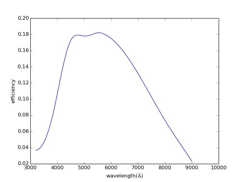
We measured the stability of flechas using an embedded Thorium-Argon (ThAr) calibration source and we find to be , at 95% confidence level over one hour.
The flechas equipped with the atik covers 31 échelle orders, as seen in Fig. 4. We measured a variable order separation from to . All orders measure about in height, exhibiting a double peak profile because of the image slicer (see Fig. 5).
The calibration in wavelength and the dispersion were obtained again by means of the ThAr lamp. The dispersion , expressed in , increases with wavelength with a linear relation of the form: , with expressed in . We found and to be and , respectively.
The spectral resolving power of flechas as a function of was determined by a Gaussian fit to the peak along the direction of dispersion (see Fig. 7), in order to measure the FWHM of the emission lines detected in the ThAr calibration spectra and averaging the FWHM over the various orders (Figs. 7 and 8).


4.3 The lhires iii spectrograph
In 2019, a Shelyak lhires iii medium-resolution was purchased. This is a long-slit spectrograph with slit width of , 1200 grooves per grism and a resolving power of according to the vendor, which will be verified in further tests, as well as the stated total efficiency of .
We decided to pair the lhires iii to the stl. In this configuration, and based on the producer’s documentation, we estimate at oarpaf a maximum observable magnitude of , for a signal-to-noise ratio of and 1 hour exposure. We also calculate a mean sampling of about , which in turn yields a mean field width of one acquisition[12] of . A micro-metric screw allows the shift of the central wavelength, so that most of the wavelength range of the stl can be in principle covered with two exposures. The Shelyak spectrograph has not been fully commissioned yet: its calibration and first usage will be presented in a different publication. We foresee the slit length on the sky to have the same size of the photometric field, so .
5 Calibrations
The calibration procedure is mainly intended to remove additive contributions to the background, such as the electronic pedestal level, the dark current, the multiplicative gain, and illumination variations across the chip. The goal of the data reduction pipeline is ideally to remove signatures of experimental distortions from the data, thus allowing us to achieve the most accurate values for the observable and to minimize the contribution of deterministic factors in the uncertainties and, at the same time, by preserving information about noise sources, so that users can evaluate the random uncertainties of the reduced data. The raw counts of a pixel in position in a CCD frame can be computed as , where is the bias value of each pixel, is the integration time, is the dark current, here expressed in ADU/pixel/s, is the sensitivity gain and is the light flux reaching the pixel including the signal from the source as well as the sky background, while is the readout noise and any other irreducible noise source of the pixels, to include information on dead or hot pixels. , and are measured from bias, dark and flat frames, respectively.
Bias frames measure the readout noise and correspond to observations without exposure to light (shutter closed) for a total integration time of 0 seconds: several frames are acquired so that a median frame can be determined with reduced statistical uncertainty. This master frame is subtracted from data during reduction. If we allow the CCD to integrate for some amount of time, without any light falling on it, there will be a signal caused by thermal excitation of electrons in the CCD: this is called dark signal and it is very sensitive to temperature.
All CCDs have non-uniformities, that is, a uniform illumination of the CCD does not yield an equal signal in each pixel (even ignoring noise). Small scale (pixel to pixel) non-uniformities (typically a few percent from one pixel to the next) are caused by slight differences in pixel sizes. Larger scale (over large fractions of the chip) non uniformities are caused by various effects, such as small variations in the silicon thickness across the chip, non-uniform illumination caused by telescope optics (vignetting). These can sum up to variations of around 10% over the chip. To measure and correct for these non-uniformities, the entire CCD is illuminated by a uniform source of light and flat field data are taken. At oarpaf, the twilight method [13] has been applied in order to acquire sky flats for photometry. The new dome also provides a setup for dome flat fields, which will be used as a backup solution.
6 Data reduction pipeline
A Python pipeline has been developed to remove the various background sources and derive a pre-treated image, as shown in Fig. 9. The development of the pipeline also foresees field solving by querying astrometry.net, and matching sources from the GAIA DR2 catalog [14, 15] in order to perform automatic aperture photometry. Field solving also overcomes errors due to the possibility of low tracking accuracy, especially on derotation. If this happens, light from a given object will not populate the same pixel for each frame. Further implementation foresees the use of a separate, on-axis guiding camera and the tip-tilt lens corrector in order to correct the pointing during frame acquisition.
Currently, data reduction pipeline is still under development. It produces light curves of stellar fields, in the form of ascii output, (tested on several exoplanetary transit targets) in fully-automatic mode, as well as complete pre-treated, astrometric-resolved fields in FITS format, containing a large number of derived parameters in the FITS Header, following a “ESO-like” standard. Long slit and échelle spectroscopy will be the next goals.
7 Remote control
Initially, the facility and the dome of the telescope were conceived to be operated only locally and manually. Consequently, the scientific usage of the telescope was limited. Of course, being able to remotely control the dome and the other instruments represents a huge advantage for the scientific exploitation of the telescope. Therefore, with the goal of remotely controlling it, we implemented a first modification towards an automated use of the dome by developing a Python script running on a Raspberry-PI to query the control center for position, and interacting with the dome by an Arduino platform. The necessary works to remotely control the dome started immediately, and the needed set of instruments was bought: these include a new weather station with rain-gauge, anemometer, hygrometer and thermometer, an all-sky camera, two IP webcams, and a new electronic system with an encoder directly interfaced to the interlock system.
This way, remote operators can monitor the weather and sky conditions at oarpaf and the possible presence of visitors; for the safety of the telescope, the dome will automatically close in case of bad weather and in case of prolonged absence of the Internet connection. A custom software framework under the Linux operating system was designed to manage all the parts.
Since remote operations must be fully reliable, a stable access to the Internet is mandatory. Unfortunately, the access link currently in use at oarpaf does not yet satisfy the necessary requirements of stability. Several actions for improving the overall quality-of-service and the service level agreements of the Internet connection are planned during 2021 by the Liguria Digitale companygg g https://www.liguriadigitale.it/. In the near future, the remote control of the facility will be obtained in two ways, described hereafter.
7.1 Ricerca
To date, a full remote control is not yet available. The newly installed dome was provided with a commercial control software, named Ricerca, developed by OmegaLabhh h http://atcr.altervista.org/ita/index.html, operating on Windows. Ricerca makes use of ASCOM drivers and can be used together with the telescope software to remotely manage the observatory and to monitor the system, the dome, and the detectors. The software interfaces with a hardware module called OCSIII, provided with relay control switches for the several mentioned subsystems, also including a screen and dome light for flat fields, which may be used for calibrations along with sky flat fields. This first remotization step will be completed before summer 2021, after the purchase of the required software licenses.
7.2 Web interface
To allow more flexibility in the framework for future development, a completely Linux-based custom control software is being set up. The latter uses top modern internet technologies to operate through commands given via a web browser, or script, through a web Application Programming Interfaces (API).
The development “from scratch” of the remotization framework for a recent observatory can involve modern solutions that do not need to rely on decades of hardware/software substrates. For this reason, we are considering to implement the front end interface using html and javascript languages via the popular Bootstrap 4 framework, whereas the V8-based technology node.js and mongodb are used for the server side development and storing purposes [12]. It already allows the control of the sbig cameras and the all-sky camera as a test benchmark and it will be implemented in order to monitor and control the dome and the telescope, as well as the weather station and the webcams, producing real-time images.
Moreover, it will allow controlling and scheduling public visits and scientific operations. In addition, it will be easily usable by schools for public events and outreach activities.
8 Science cases
The scientific reach of oarpaf is wide. Observations and preliminary results achieved during the past years demonstrate the large potential of the facility: these include observations for which small, -class telescopes, such as oarpaf, have enough sensitivity to be competitive for measurements that require long campaigns, typically not possible with big telescopes, whose observation time has to be shared among a number of projects.
The scientific potential of the telescope has been presented in several nationalii i http://events.iasfbo.inaf.it/gloria/od_programme.php and international conferences [2, 16, 17, 12] and in master-degree theses of students of the University of Genova [18, 19, 20].
In the following subsections we present such results and future prospects.
8.1 Exoplanetary transits
Planets orbiting stars other than the Sun have been first discovered in the 90s and along the years their number increased and passed 4000jj j http://exoplanet.eu. They can be detected with different experimental methods. For oarpaf, the photometric transit [21] is the most suitable method. To measure the needed light curves, we adopted the defocused photometry [22] allowing the star hosting the target exoplanet to cover many pixels, and to obtain magnitude dispersion levels that have been proved to be comparable to those of space telescopes in observatories of the same class of oarpaf, such as GROND or the Danish . The measurements thus obtained are practically unaffected by any instrumental defects, by calibration biases, and by variations of the quality of the observing night, an important aspect for measurements that can possibly last several hours. These results are indeed within the range of oarpaf, but further instrument setup issues, such as the star chasing or a tip tilt correction, have to be implemented.
At oarpaf, we observed, with the stl, the exoplanet TrES-3b using the defocused photometry technique. The observation contributed to a peer reviewed publication [3], where data also gathered at the Observatorio Astronomico Nacional de San Pedro Martir (Mexico), Observatorio de la Universidad de Monterrey (Mexico) and Telescopio Carlos Sanchez at the Observatorio del Teide (Spain) were combined (Fig. 10), thus allowing us to derive physical and orbital parameters of the planet. Other exoplanets that we observed include WASP-58b, HAT-P-3b and HAT-P-12b [19, 16]: the related data reduction is ongoing using the pipeline described in Sect. 6.
8.2 Active galactic nuclei
Active galactic nuclei are the most luminous persistent sources of electromagnetic radiation. Some of them display jets of relativistic particles and are named blazars when the jet points to the observer. It is possible to distinguish among various models for blazars by measuring the optical variability with long monitoring campaigns [11, 23, 24, 25, 26] . A feasibility test of such measurements has been performed in order to make sure that such sources can be observed at oarpaf. Considering all the characteristics of the telescope, the instruments, and the site, several observable blazars have been identified.
A very faint object, SDSS J223827.17+135432.6, with magnitude in the filter, could be observed (Fig. 11) with a large signal-to-noise ratio of around , with just of exposure time [18]. Other interesting blazar candidates that can be observed at oarpaf include 4C+41.11, MG1J021114+1051, PMNJ2227+0037: these are particularly interesting because they could also be emitters of very high energy neutrinos. It would be of particular interest to observe them in coincidence with observations in other bands, or , in order to derive a multiwavelength measurement.
For a QSO with magnitude 20, we can achieve a precision in magnitude with an exposure time of around : this was enough for the planned measurements. In the same conditions and with the same set up, achieving an uncertainty of mag may require an exposure time a factor 100 longer, which is not sustainable. However, using the stx, integrated with the AO-X system, we can improve the sensitivity: this is a possibility may be explored for measurements requiring a better precision on the magnitude.
8.3 Gravitationally lensed quasars
When a galaxy or cluster of galaxies lies between a far away quasar and the observer, it produces strong gravitational lensing: multiple images of the source quasar are observed. Since quasars typically feature variation in luminosity and color[27, 28], the various multiple images of the source show the same features in the light curve, with a time delay due to the different paths the photons travelled due to the presence of the lensing galaxy or galaxy cluster.
Time delays of gravitationally lensed quasars allows measuring the Hubble parameter [29, 30] : long campaigns, lasting years, are needed to derive time delays [31]. The feasibility of such measurements at oarpaf has been demonstrated by observing the two lensed quasars SDSS J1004+4112 and QSO 0957+561 [20], the latter shown in Fig. 12. The first is particularly suitable because it can be observed during most of the year in Northern Italy, it has a relatively large magnitude, around 18 in the band, and it features a large angular separation between the multiple images, –, permitting to easily separate and reconstruct the light curves of each image.
A novel experimental method to enhance the number of usable lensed quasarskk k A. Domi, et al., “A novel method to measure time delay of not resolved gravitationally-lensed quasars using source color variations”, in preparation. for time delay measurements by class telescope has been elaborated [20]. A collaboration with theorists of the University of Genoa has been established aimed at studying possible improvements to the relation between time delay and the Hubble parameter from a theoretical and phenomenological point of view [32, 33].
8.4 Microlensing
oarpaf is potentially suited for microlensing studies. In particular, microlensing searches can be divided into two main categories with different final goals, briefly explained hereafter.
- •
Planetary microlensing: the crowded the stellar field, the higher the probability to detect a microlensing event. The best sky regions for this activity are the galactic bulge and the Magellanic clouds, which are not accessible at oarpaf. Although, a derived technique called pixel lensing[34] can be applied in unresolved star regions such as the Andromeda galaxy. The use of the AO-X module with the stx to stabilize the image can be promising in this kind of research topic.
- •
Quasar microlensing: strongly lensed quasars, described in Sect. 8.3, are affected by the microlensing phenomenon. Specifically, massive objects in the lensing galaxy, such as stars, impact the observed multiple images of the quasar source in the form of sharp and uncorrelated brightness variations. These brightness changes are associated with the light coming from the innermost region of the quasar, passing through a pattern of caustics produced by massive objects in the lensing galaxy. It has been demonstrated [35] that microlensing provides a unique and direct observation of the internal structure of the lensed quasar. Such measurement relies on the temporal variation of high-magnification caustic crossings which vary on timescales of days to years. Moreover, multiwavelength observations provide information from distinct emission regions in the quasar. Therefore, the monitoring of strongly lensed quasars also in terms of microlensing represents a unique and comprehensive probe of active black hole structure and dynamics. This method requires resolved multiple images of the quasar. Therefore, even though this condition reduces the observational sample of the oarpaf telescope, it is still a possible measurement with resolved systems such as the ones already observed and cited in Sect. 8.3.
8.5 Asteroids

The study of objects in the asteroid belt is an interesting branch of astronomy due to the relative vicinity of such targets and the uncertainty on several of their properties and orbital parameters ll l https://nssdc.gsfc.nasa.gov/planetary/planets/asteroidpage.html. It is particularly interesting to measure light curves of the asteroids when they are in opposition, as this is the most favored configuration. Simplifying the object as an ellipsoid with 3 axes, one assumes that luminosity variations are only due to the orientation of the rotation pole with respect to the ecliptic and the shape of the ellipsoid. With good quality photometric observations, one can measure both the orientation of the rotation axis and the ratio between the major semiaxes of the ellipsoid [36]. In particular, we plan to observe the asteroid 1671 Chaika [37]: it is particularly suitable for oarpaf because of its large apparent luminosity and interesting orbital features.
9 Teaching and outreach
Since the beginning, events for schools and the general public have been organized at oarpaf, and had a big success. The astrophile association Urania is in charge of events for primary school kids and the citizens, while ORSA manages events for high-school and University students. So far, only events requiring the physical presence at the Observatory have been organized because the telescope can only be operated in local mode.
Data taken with the telescope have been used for teaching purposes in events for high school and third age students and pictures taken with the telescope have been shown in various events and festivals. Several students of the faculty of physics made use of the telescope and its instruments to perform their master degree theses, actually greatly contributing to the commissioning and the verification of the scientific potential [18, 19, 20]. We expect that, when the facility will be operated remotely, the number of events and the number of participants will significantly increase and it will also involve potential users of other time zones.
10 Conclusions
We presented the oarpaf observatory and its instrumentation. With
the current setup, we measure a plate scale of
, a pointing accuracy is of
rms, and a tracking accuracy of .
We find for the three available detectors a good linearity range
(approximately from 4 000 to above 60 000), and we give an
estimation of the gain and the dark current.
The typical brightness at oarpaf is found to be
in the filter, down to
in the filter, while the seeing
spans between – with a typical value of
.
Extinction coefficient and zero points are also calculated by the
observation of standard stars.
oarpaf instrumentation also includes an échelle and a long slit spectrograph. We find for the échelle spectrograph a order stability of , at 95% confidence level over one hour, a dispersion of the 31 orders between – with a width of and . The commissioning of the long slit spectrograph is in progress.
We foresee that the implementation of the remotization process, of the instrumentation setup, and of the scientific operations will give a valuable contribution in cutting-edge scientific topics, such as the search for exoplanets, the observation of AGNs (these two already leading to peer-reviewed publications), the measurement of gravitationally lensed quasars time delays and the study of asteroids.
Thanks to its great potential, the funding needed for the complete remotization of the facility has been obtained. Therefore, oarpaf is expected to fully operate remotely by end of 2021.
Acknowledgments
We thank the University of Genova for the financial, administrative and logistic support, in particular dr. W. Riva of the central administration, as well as all members of ORSA and the students of DIFI for their enthusiasm. We thank R. Cereseto, M. Cresta and E. Vigo of the mechanical and electronic services of DIFI and INFN-Sezione di Genova for the technical interventions on the engines of the eye of the original dome. We thank the theorists N. Alchera, M. Bonici, N. Maggiore and L. Panizzi for useful discussions and ideas, as well as C. Ayala-Loera and S. Brown-Sevilla for the collaboration with measurements of exoplanetary transits. We are grateful to L. Nicastro and E. Palazzi from INAF-OAS for their help in the beginning of the operations. We thank the Astelco Systems company for the always helpful feedback. We are deeply appreciative to Associazione Urania who made it possible to transform the dream of an observatory on the Ligurian Apennines in reality. And, of course, we deeply thank Regione Liguria, Comune di Fascia and Ente Parco Antola for the always fruitful collaboration. Fundings for the facility and instruments were provided by Regione Liguria, Programma Italia-Francia Marittimo, Comune di Fascia, Ente Parco Antola, Università di Genova, DIFI and DIBRIS,MIUR Progetto Dipartimenti di Eccellenza. Instruments for outreach events and activities for students received contributions by Piano Lauree Scientifiche (PLS) of MIUR. Individuals have received support by INAF, INFN and MIUR (FFABR). Finally, we thank the editor and the anonymous referees, whose remarks contributed to improve the paper.
References
- [1] A. Federici, P. Arduino, A. Riva, et al., “The Antola Public Observatory: a newborn European facility,” in Astronomical Society of India Conference Series, Astronomical Society of India Conference Series 7, 7 (2012).
- [2] C. Righi, “Extrasolar and Bl Lac observations at OARPAF,” Nuovo Cimento C Geophysics Space Physics C 39, 284 (2016).
- [3] D. Ricci, P. V. Sada, S. Navarro-Meza, et al., “Multi-filter Transit Observations of HAT-P-3b and TrES-3b with Multiple Northern Hemisphere Telescopes,” PASP 129, 064401 (2017).
- [4] C. E. Cramer, K. R. Lykke, J. T. Woodward, et al., “Precise measurement of lunar spectral irradiance at visible wavelengths,” Journal of research of the National Institute of Standards and Technology 118, 396–402 (2013).
- [5] A. M. Jones, S. Noll, W. Kausch, et al., “An Advanced Scattered Moonlight Model,” The Messenger 156, 31–34 (2014).
- [6] P. B. Stetson, “Some factors affecting the accuracy of stellar photometry with ccds (and some ways of dealing with them),” Highlights of Astronomy 8, 635–644 (1989).
- [7] S. B. Howell, Handbook of CCD Astronomy, Cambridge University Press (2000).
- [8] M. B. Taylor, “TOPCAT & STIL: Starlink Table/VOTable Processing Software,” in Astronomical Data Analysis Software and Systems XIV, P. Shopbell, M. Britton, and R. Ebert, Eds., Astronomical Society of the Pacific Conference Series 347, 29 (2005).
- [9] M. S. Bessell, “UBVRI passbands.,” PASP 102, 1181–1199 (1990).
- [10] L. Cabona, D. Ricci, A. Marini, et al., “Cerberus: A three-headed instrument for the OARPAF telescope,” in Society of Photo-Optical Instrumentation Engineers (SPIE) Conference Series, Society of Photo-Optical Instrumentation Engineers (SPIE) Conference Series 11447, 114475J (2020).
- [11] M. Mugrauer, G. Avila, and C. Guirao, “FLECHAS - A new échelle spectrograph at the University Observatory Jena,” Astronomische Nachrichten 335, 417 (2014).
- [12] D. Ricci, L. Cabona, A. La Camera, et al., “Technical and software upgrades completed and planned at OARPAF,” (2020).
- [13] N. D. Tyson and R. R. Gal, “An Exposure Guide for Taking Twilight Flatfields With large Format CCDs,” AJ 105, 1206 (1993).
- [14] Gaia Collaboration, T. Prusti, J. H. J. de Bruijne, et al., “The Gaia mission,” A&A 595, A1 (2016).
- [15] Gaia Collaboration, A. G. A. Brown, A. Vallenari, et al., “Gaia Data Release 2. Summary of the contents and survey properties,” A&A 616, A1 (2018).
- [16] L. Cabona, “Commissioning and photometry at the OARPAF,” in ChiantiTopics, 2nd International Focus Workshop, 2016, Use of small telescopes in the giant era 2 (2016).
- [17] D. Ricci, “Multi-filter, multi-telescope exoplanetary transit observations,” in ChiantiTopics, 2nd International Focus Workshop, 2016, Use of small telescopes in the giant era 2 (2016).
- [18] C. Righi, “Photometric variability of weak emission line quasars. a tool for understanding the actual nature of the source: blazar or qso? from instrument calibrations to science,” Master’s thesis, Università di Genova, Italy (2015).
- [19] L. Cabona, “Commissioning of the antola observatory. determination of the performances of the spectrograph and a first scientific measurement: observation of exoplanet transits,” Master’s thesis, Università di Genova, Italy (2016).
- [20] F. Nicolosi, “Commissioning of the instrumentation of OARPAF and applications to the photometry of gravitational lenses,” Master’s thesis, Università di Genova, Italy (2019).
- [21] D. Charbonneau, T. M. Brown, D. W. Latham, et al., “Detection of Planetary Transits Across a Sun-like Star,” ApJ 529, L45–L48 (2000).
- [22] J. Southworth, L. Mancini, P. Browne, et al., “High-precision photometry by telescope defocusing - V. WASP-15 and WASP-16,” MNRAS 434, 1300–1308 (2013).
- [23] T. A. Rector, J. T. Stocke, E. S. Perlman, et al., “The Properties of the X-Ray-selected EMSS Sample of BL Lacertae Objects,” AJ 120, 1626–1647 (2000).
- [24] T. A. Rector and J. T. Stocke, “The Properties of the Radio-Selected 1 Jy Sample of BL Lacertae Objects,” AJ 122, 565–584 (2001).
- [25] P. Padovani, P. Giommi, H. Landt, et al., “The Deep X-Ray Radio Blazar Survey. III. Radio Number Counts, Evolutionary Properties, and Luminosity Function of Blazars,” ApJ 662, 182–198 (2007).
- [26] P. Giommi, P. Padovani, G. Polenta, et al., “A simplified view of blazars: clearing the fog around long-standing selection effects,” MNRAS 420, 2899–2911 (2012).
- [27] D. Ricci, J. Poels, A. Elyiv, et al., “Flux and color variations of the quadruply imaged quasar HE 0435-1223,” A&A 528, A42 (2011).
- [28] D. Ricci, A. Elyiv, F. Finet, et al., “Flux and color variations of the doubly imaged quasar UM673,” A&A 551, A104 (2013).
- [29] S. Refsdal, “The gravitational lens effect,” MNRAS 128, 295 (1964).
- [30] S. H. Suyu, V. Bonvin, F. Courbin, et al., “H0LiCOW - I. H0 Lenses in COSMOGRAIL’s Wellspring: program overview,” MNRAS 468, 2590–2604 (2017).
- [31] A. Eigenbrod, F. Courbin, C. Vuissoz, et al., “COSMOGRAIL: The COSmological MOnitoring of GRAvItational Lenses. I. How to sample the light curves of gravitationally lensed quasars to measure accurate time delays,” A&A 436, 25–35 (2005).
- [32] N. Alchera, M. Bonici, and N. Maggiore, “Towards a new proposal for the time delay in gravitational lensing,” Symmetry 9, 202 (2017).
- [33] N. Alchera, M. Bonici, R. Cardinale, et al., “Analysis of the angular dependence of time delay in gravitational lensing,” Symmetry 10, 246 (2018).
- [34] S. Calchi Novati, “Pixel lensing. Microlensing towards M31,” General Relativity and Gravitation 42, 2101–2126 (2010).
- [35] L. Moustakas, M. O’Dowd, T. Anguita, et al., “Astro2020 science white paper - quasar microlensing: Revolutionizing our understanding of quasar structure and dynamics,” (2019).
- [36] A. Pospieszalska-Surdej and J. Surdej, “Determination of the pole orientation of an asteroid - The amplitude-aspect relation revisited,” A&A 149, 186–194 (1985).
- [37] A. Mainzer, T. Grav, J. Masiero, et al., “NEOWISE Studies of Spectrophotometrically Classified Asteroids: Preliminary Results,” ApJ 741, 90 (2011).
List of Tables
table.caption.3subtable.1.1subtable.1.2
List of Figures
figure.caption.1figure.caption.2figure.caption.4figure.caption.5figure.caption.6figure.caption.7figure.caption.8figure.caption.9figure.caption.10figure.caption.11figure.caption.12figure.caption.13