Distinguishing limit of Bell states for any $n$-photon $D$-dimensional hyperentanglementPreprint: APS/123-QED

Bell state measurement (BSM) is a crucial measurement in quantum mechanics, using joint orthogonal projection measurement. It enables many applications in quantum information processing, such as superdense coding (SDC) Bennett and Wiesner 1992; Mattle et al. 1996, teleportation Bennett et al. 1993; Bouwmeester et al. 1997; Boschi et al. 1998, entanglement swapping Zukowski et al. 1993; Pan et al. 1998 and quantum finger printing Buhrman et al. 2001; Horn et al. 2005. An important parameter of the quantum communication is a channel capacity (CC), which is determined by the number of distinguished Bell states by BSM Barreiro et al. 2008. However, a complete BSM with linear optics is impossible Vaidman and Yoran 1999; Lütkenhaus et al. 1999 and its optimal probability of success is only 50% Lütkenhaus et al. 1999; Calsamiglia and Lütkenhaus 2000; Calsamiglia 2002. In other words, there is an upper bound of CC for any given entangled system. As a result, the rate of quantum information between a sender (Alice) and a receiver (Bob) is limited. Many attempts have been made to establish optimal BSM schemes and achieve their limits using high-dimensional entanglement in both theory and experiments Hu et al. 2018; Wei et al. 2007; Pisenti et al. 2011; Kong et al. 2019a.

Actually, high-dimensional entanglement has many advantages over two-qubit entanglement, such as higher CC Liu et al. 2002; Grudka and Wójcik 2002 and transmission rate Cerf et al. 2002; Bruss and Macchiavello 2002. It is indeed effective to completely distinguish more than four Bell state using hybrid degrees of freedom (DOFs), such as path Hu et al. 2018 and orbital angular momentum (OAM) Kong et al. 2019b, which is called hyperentanglement. Recently, other similar BSM schemes of hyperentanglement have been demonstrated in various optical systems Dada et al. 2011; Schaeff et al. 2015; Krenn et al. 2014; Kues et al. 2017. Some special cases were proved in theory and demonstrated by experiments. Wei et al. theoretically presented that the optimal scheme divides 16 Bell states into 7 distinct groups Wei et al. 2007. Pisenti et al. showed that at most $2^{n+1}-1$ classes out of $4^{n}$ hyperentangled Bell states can be distinguished with one copy of input states Pisenti et al. 2011. Hu et al. gave a four-dimensional entanglement protocol, which exceeded the channel capacity limit of 2 for the first time Hu et al. 2018. Kong et al. produced eight eight-dimensional Bell-like states and distinguished them completely Kong et al. 2019a. This is because adding additional DOFs also enlarges Hilbert space and hence the number of Bell-like states also increases. However it is interesting and necessary for practice that what is the theoretical limit for distinguished Bell states in Hilbert space.

In our paper, we firstly investigate the distinguishing limit $N$ of Bell states for any $n$-photon $D$-dimensional hyperentangled system ($nD$ system). To achieve this, for all kinds of unitary transformation $U$ in the input-output relation $\vec{c}=U\vec{a}$ for any linear-optics circuits, we separate them into two groups using a norm ($G_{1}$ and $G_{2}$) Pisenti et al. 2011. With the help of Pisenti’s work Pisenti et al. 2011, we extend the method to $n$-photon systems and find that the limit for $G_{1}$ is ${N_{1}}=nD-(n-1)$. We also verify this result using Peter van Loock and Norbert Lütkenhaus’s criterion (LL criterion) van Loock and Lütkenhaus 2006. This limit can not only apply to bosons’ entanglement, but fermions’ as well. For the second group of $U$ ($G_{2}$) we infer that at least $D^{n-1}$ Bell states can be distinguished for any $nD$ system due to the symmetry of Bell states and the limit for $G_{2}$ is ${N_{2}}\geq{D^{n-1}}$. The BSM scheme for a four-photon two-dimensional system with $G_{2}=E$ ($E$ is the identity matrix) has been illustrated. It is clearly that for any entangled system with $n>2$, ${N_{1}}\leq{N_{2}}$. Finally, we report an experimental demonstration theoretically for two-photon eight-dimensional hyperentanglement using spin, path and the first order of OAM, based on Kong’s Kong et al. 2019a and Hu’s Hu et al. 2018 work. 64 Bell states can be divided into 15 different classes, which achieves CC’s upper limit ${\log_{2}}15$ for this case.

The $D$-dimensional Bell basis of an $n$-particle system can be written as Liu et al. 2002:

where $P,j,{i_{1}},{i_{2}},...,{i_{n-1}}=0,1,...,D-1$. We define the vectors $\vec{a}=(\hat{a}_{{{1}}}^{\dagger},\hat{a}_{{{2}}}^{\dagger},\cdots,\hat{a}_{{{nD}}}^{\dagger})^{T}$ and $\vec{c}=(\hat{c}_{{{1}}}^{\dagger},\hat{c}_{{{2}}}^{\dagger},\cdots,\hat{c}_{{{nD}}}^{\dagger})^{T}$, where $\hat{a}_{{{i}}}^{\dagger}$ and $\hat{c}_{{{i}}}^{\dagger}$ represent an input and an output mode separately. Then linear-optics devices functioning as the unitary matrix $U$ in the circuits transform $\vec{a}$ to $\vec{c}$ follow the input-output relation $\vec{c}=U\vec{a}$. If the arbitrary initial $n$-particle Bell state is $\left|{{\varphi_{j}}}\right\rangle$, the state following $n-1$ clicks in some detectors is proportional to ${\hat{c}_{{s_{n-1}}}}\cdots{\hat{c}_{{s_{2}}}}{\hat{c}_{{s_{1}}}}\left|{{\varphi_{j}}}\right\rangle$, where $\hat{c}_{{{s_{i}}}}$ ($s_{i}=1,2,\ldots,nD$) is the annihilation operator associated with corresponding output mode. We call these states post-click states. Then we can separate all kinds of $U$ into two groups, $G_{1}$ and $G_{2}$, by the result of the norm of the post-click states with $n-1$ clicks $\left\langle{{\varphi_{j}}}\right|\hat{c}_{{s_{1}}}^{\dagger}\hat{c}_{{s_{2}}}^{\dagger}\cdots\hat{c}_{{s_{n-1}}}^{\dagger}{\hat{c}_{{s_{n-1}}}}\cdots{\hat{c}_{{s_{2}}}}{\hat{c}_{{s_{1}}}}\left|{{\varphi_{j}}}\right\rangle$. The norm shows the probability of $n-1$ clicks in the corresponding detectors, where we can easily find that the norm is nonnegative.

To define $G_{1}$, the norm for any combination of ${\hat{c}_{{s_{i}}}}$ and $\left|{{\varphi_{j}}}\right\rangle$ is nonzero. At this time, all the unitary matrices $U$ in $G_{1}$ must satisfy Eq. (2)

where when ${{\hat{a}}_{{p_{1}}}}{{\hat{a}}_{{p_{2}}}}\cdots{{\hat{a}}_{{p_{n-1}}}}={{\hat{a}}_{{q_{1}}}}{{\hat{a}}_{{q_{2}}}}\cdots{{\hat{a}}_{{q_{n-1}}}}$, $\left\langle{{\varphi_{j}}}\right|\hat{a}_{{p_{1}}}^{\dagger}\hat{a}_{{p_{2}}}^{\dagger}\cdots\hat{a}_{{p_{n-1}}}^{\dagger}{{\hat{a}}_{{q_{n-1}}}}\cdots{{\hat{a}}_{{q_{2}}}}{{\hat{a}}_{{q_{1}}}}\left|{{\varphi_{j}}}\right\rangle$ can be nonzero. This nonzero result means that via $G_{1}$, every Bell state is capable of producing $n-1$ clicks in all detectors randomly, but these detector clicks provide nothing about which Bell state particles occupy. In other words, the last click will determine the distinguishing of Bell states. Thus, we can get the distinguishing limit $N_{1}$ by analysing all the Bell state’s last click to simplify the problem.

To define $G_{2}$, on the contrary, the norm for some combinations of ${\hat{c}_{{s_{i}}}}$ and $\left|{{\varphi_{j}}}\right\rangle$ is zero. For instance, identity matrices belong to $G_{2}$. In other words, when $\vec{c}=\vec{a}$, we can easily derive from Eq. (1) that the norm $\left\langle{{\varphi_{j}}}\right|\hat{a}_{{s_{1}}}^{\dagger}\hat{a}_{{s_{2}}}^{\dagger}\cdots\hat{a}_{{s_{n-1}}}^{\dagger}{\hat{a}_{{s_{n-1}}}}\cdots{\hat{a}_{{s_{2}}}}{\hat{a}_{{s_{1}}}}\left|{{\varphi_{j}}}\right\rangle$ for some combination of ${\hat{a}_{{s_{i}}}}$ and $\left|{{\varphi_{j}}}\right\rangle$ is zero. Thus for $G_{2}$ we cannot simplify the problem as the case of $G_{1}$ and more discussion on $G_{2}$ is shown at the end of this section.

With $G_{1}$, we can derive $N_{1}$ for any $nD$ system by generalizing Pisenti’s method for two-photon systems Pisenti et al. 2011. Firstly, we define every output mode $\hat{c}_{{i}}^{\dagger}$ $(i=1,2,\ldots,nD)$ corresponds to a detector mode $\left|{{D_{i}}}\right\rangle$, which takes the form as follows

where ${\hat{b}^{\dagger}}_{{i_{j}}}$ must come from $n$ different particles and ${\hat{b}^{\dagger}}_{{i_{j}}}\left|0\right\rangle$ is a superposition of the $j^{\text{th}}$-particle’s input state. We define the detection signature as ${P_{12\ldots n}}\left|{{D_{{i_{1}}}}}\right\rangle\left|{{D_{{i_{2}}}}}\right\rangle\ldots\left|{{D_{{i_{n}}}}}\right\rangle$ Pisenti et al. 2011. The projection operator ${P_{12\ldots n}}$ projects the raw tensor product of $n$ detector modes $\left|{{D_{{i_{1}}}}}\right\rangle\left|{{D_{{i_{2}}}}}\right\rangle\ldots\left|{{D_{{i_{n}}}}}\right\rangle$ onto the subspace of $n$-particle states, which makes sure the modes come from different particles. Since every Bell state can be represented by an independent detection signature (IDS), the number of IDS equals to that of distinguishable Bell states.

For two-particle $D$-dimensional hyperentangled systems, the norm Eq. (2) is always positive Pisenti et al. 2011. All kinds of $U$ are in $G_{1}$ here, thus there are $2D$ detection signatures with the post-click states with one click. Following Pisenti’s method Pisenti et al. 2011, the number of IDS is $2D-1$ for both bosons and fermions cases. When we just consider ${m}$ qubitlike degrees of freedom on each photon, $D={2^{{m}}}$ and ${N_{1}}={2^{{m}+1}}-1$, which is just the same as Pisenti’s result Pisenti et al. 2011.

When we extend Pisenti’s method Pisenti et al. 2011 to $nD$ systems with $G_{1}$ and consider the post-click states with $n-1$ clicks, there are $nD$ detection signatures. For bosons with three-photon $D$-dimensional entanglement, there are $3D$ detection signatures if considering the post-click states with the first two clicks in $D_{i}$ as $\left|{{D_{i}}}\right\rangle\left|{{D_{i}}}\right\rangle=({\alpha_{{i_{1}}}}{{\hat{b}}^{\dagger}}_{{i_{1}}}+{\alpha_{{i_{2}}}}{{\hat{b}}^{\dagger}}_{{i_{2}}}+{\alpha_{{i_{3}}}}{{\hat{b}}^{\dagger}}_{{i_{3}}})^{2}\left|00\right\rangle$. However, these $3D$ detection signatures are not independent. Next, we will show that there are only two independent constraint equations among them. Firstly, we can always find some linear combination of detector modes satisfy

then we have ${P_{123}}\left|{{D_{i}}}\right\rangle\left|{{D_{i}}}\right\rangle\left|{{X}}\right\rangle=0$ if and only if $B+C=-1$. For example,

In the three-dimensional Vector space, $\vec{v}_{1}=(1,-\frac{1}{2},-\frac{1}{2})$ and $\vec{v}_{2}=(1,-\frac{1}{3},-\frac{2}{3})$ are linearly independent. Since $\vec{v}_{3}=(1,B,-1-B)$ is on the plane made up of $\vec{v}_{1}$ and $\vec{v}_{2}$, $\vec{v}_{3}$ can be represented by $\vec{v}_{1}$ and $\vec{v}_{2}$ for any constant $B$. In other words, any $\left|X\right\rangle$ satisfying ${P_{123}}\left|{{D_{{i}}}}\right\rangle\left|{{D_{{i}}}}\right\rangle\left|{{X}}\right\rangle=0$ can be represented by $\left|{{X_{1}}}\right\rangle$ and $\left|{{X_{2}}}\right\rangle$. Thus there are only two independent constraint equations, and they are

The last click in detectors matters to distinguish Bell states with $G_{1}$, whether the first two detector modes are the same or not. Therefore, the number of IDS is at most $3D-2$. Similarly, there are $nD$ detection signatures for $nD$ systems with post-click states with $n-1$ detector clicks. But we can always find $n-1$ independent constraint equations, so the number of IDS in this case is

Here, we note that we cannot completely distinguish $N_{1}$ Bell states of $nD$ system without number-resolving detectors.

For Fermions, anti-symmetry under particle exchange is a must. Thus, $n$ clicks must trigger $n$ different detectors to get allowed post-click states. For the post-click states with $n-1$ different clicks, the last click has only $nD-(n-1)$ possibilities. That is to say, there are at most $nD-(n-1)$ detection signatures as well as the number of IDS.

We also verify this result by LL criterion. It shows that the set of necessary and sufficient conditions for complete discrimination between two states $\left|{{\varphi_{i}}}\right\rangle$ and $\left|{{\varphi_{j}}}\right\rangle$ $(i\neq j)$ with linear optics are van Loock and Lütkenhaus 2006:

Because the norm Eq. (2) is nonzero with $G_{1}$, different output mode operators in Eq. (8) can be all substituted with a particular mode operator ${\hat{c}_{s}}$, shown as Eq. (9),

Actually, using Eq. (9) with $m=n-1$, we can simply derive the result ${N_{1}}=nD-(n-1)$ by summarizing the results of many $nD$ systems. Here we show the distinguishing limit of some specific systems with the help of LL criterion in TABLE 1.

When it comes to $G_{2}$, the number of detection signatures cannot be calculated simply and Eq. (9) is not a necessary and sufficient condition any more. But we can still easily distinguish $D^{n-1}$ Bell states with $U=E$ due to Bell-state symmetry. As shown in Fig.1, for the four-photon two-dimensional BSM scheme using spin, each PBS act as an identity matrix $E$ to transform the input mode ${{\hat{a}}^{\dagger}}_{i}$ to the detector mode $\left|{{D_{i}}}\right\rangle$. We can easily distinguish $8$ Bell states due to the symmetry. For the $nD$ system, we can similarly use some linear-optics devices functioning as $U_{p_{i}}=E_{i}$ like PBS. Therefore, $D^{n-1}$ Bell states can be distinguished completely with $G_{2}=E$ due to the symmetry.

Comparing with the case of $G_{1}$ mentioned above, it is clearly that $N_{1}\leq N_{2}$ for any entangled system with $n>2$. The equality sign holds if and only if $N_{2}=D^{n-1}$, $n=3$ and $D=2$. In addition, in two-photon systems measurement efficiency ${\rm{ME}}=\frac{{2D-1}}{{{D^{2}}}}$, and in multi-photon systems ${\rm{ME}}\geq\frac{1}{D}$. Except two-photon two-dimensional systems, all the other two-photon systems’ ME is less than $\frac{1}{2}$. While for multi-photon two-dimensional systems, ME is at least $\frac{1}{2}$. Thus, we can come to the conclusion that high-dimensional multi-photon hyperentanglement with $G_{2}$ circuits has great potential to achieve high CC and ME at the same time.

In the theory section, we have analyzed the optimal BSM schemes in different quantum systems. For a two-particle eight-dimensional hyperentangled system, $N_{1}=15$. Kong et al. experimentally achieved the complete distinction of eight Bell-like states using linear optical elements Kong et al. 2019a, which did not achieve the distinguishing limit of this system. Thus, in this section, we would present an eight-dimensional BSM scheme theoretically based on two-photon OAM-spin-path hyperentanglement Barreiro et al. 2005 composed of two-dimensional OAM ($\pm 1$ order), spin and path, which distinguishes 15 Bell-like states completely.

First, 15 two-photon Bell-like states we are to focus on can be formulated as

Here spin, path and OAM Bell states are defined respectively as

Here $H$($V$) represents the horizontal (vertical) polarization, $a_{1}$ and $a_{2}$ ($a_{3}$ and $a_{4}$) represents two different paths for photon A (B), $\left|{+1}\right\rangle$ ($\left|{-1}\right\rangle$) denotes a state of photon with an OAM of $+\hbar$ ($-\hbar$). All the 15 Bell-like states showed in Eq.(III) are in identical eight-dimensional Hilbert space. We perform unitary operation ${U^{O}}\otimes{U^{S}}\otimes{U^{P}}$ on the state $\left|{{\Phi_{1}}}\right\rangle$ of photon A to prepare the 15 Bell-like states described in Eq. (III) (Fig. 2)

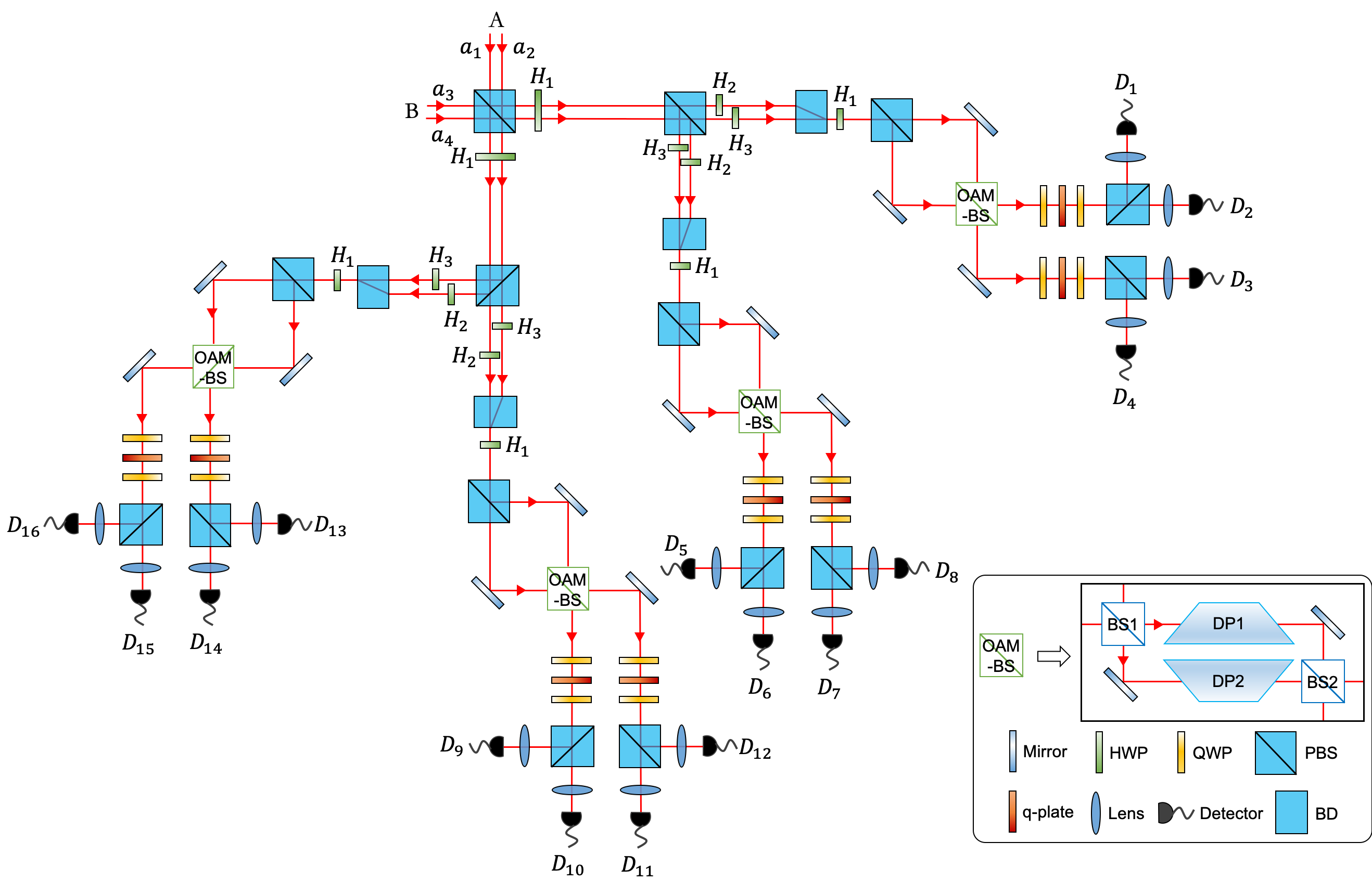
In order to unambiguously distinguish 15 Bell-like states mentioned in Eq. (III), we design a theoretical optimal BSM scheme based on Hu’s Hu et al. 2018 and Kong’s work Kong et al. 2019a (Fig. 3). Only linear optical elements such as PBS, HWP, QWP, q-plate, DP (Dove prism) BS (beam splitter) and BD (beam displacer) are used.

According to this experimental setup (Fig. 3), we can derive the coincidence between detectors for 15 Bell-like states in Eq. (III) (Fig. 4A) and classify all 64 Bell-like states into 15 different classes (Fig. 4B). The results show that any one of the 15 Bell-like states have a unique pattern of coincidence between detectors. That is to say, all these Bell-like states can be distinguished completely. This result corresponds to the theory in the previous section, since the independent constraint equation here is ${P_{12}}\left|{{D_{1}}}\right\rangle\left|{{D_{8}}}\right\rangle{\rm{=}}0$. Moreover, it is worthy to note that $\left|{{\Phi_{49}}}\right\rangle$ has 16 two-fold coincidence between the same detector. Thus, one can distinguish 14 classes of Bell-like states without number-resolving detectors.

Here we want to further discuss the meaning of our experiment. Just as the experiment shows, if we want to realize an optimal BSM for two-photon systems experimentally, mixing particles in their channels is a must. For instance, in the decode (Bob) part in our experiment, the two laser beams go into the same PBS from different directions at first. This is the key to success. As a result, every single photon has chance to trigger every single detector. Thus, there are more possibilities for the coincidences between detectors. So as to the projective basis in the experiment. So, more classes of Bell states can be distinguished in the end. According to Pisenti’s results Pisenti et al. 2011, when n particles are mixed, the upper limit is $nD$ when we ignore the constraint part. If not mixed, the same bound can reduce to only $D$. Take Kong’s Kong et al. 2019a and Hu’s Hu et al. 2018 work for examples. Hu’s work can realize an optimal BSM theoretically, and the setup has the feature on PBS corresponding to the discussion above. Compared with Hu’s setup, Kong’s setup split the pump into two beams and each of them passes through a Bell-like state analyzer separately. Therefore, it lacks the coincidences between the detectors from the same Bell-like state analyzer and only 8 Bell-like states can be distinguished from 64 ones.

In summary, we have obtained the distinguishing limit $N$ for any $nD$ entangled system. For those linear-optics circuits with $G_{1}$, we have proved that ${N_{1}}=nD-(n-1)$ , which can be applied to both bosons’ and fermions’ cases. It is worth mentioning that being different from multi-photon systems, ${N_{1}}=2D-1$ is the upper limit for two-photon systems. For those circuits with $G_{2}$, we infer that ${N_{2}}\geq{D^{n-1}}$ due to the symmetry of Bell states. Thus, for those $n$-photon entangled systems with $n>2$, one can at least distinguish $D^{n-1}$ Bell states with optimal BSM schemes. We also verify the result for $N_{1}$ using LL criterion. Particularly, since for those circuits with $G_{1}$ the norm Eq. (2) is always positive, we have proved that Eq. (9) is a sufficient and necessary condition to distinguish two states here. This can help largely reduce and simplify the computation. Based on this result, we can choose a better entangled system to realize BSM effectively and check quickly if any given BSM scheme has reached the limit $N$. Moreover, we have demonstrated the BSM scheme theoretically for two-photon eight-dimensional hyperentanglement using spin, path and the first order of OAM, based on Kong’s Kong et al. 2019a and Hu’s Hu et al. 2018 work. The highlight is this scheme helps to achieve the CC’s upper bound ${\log_{2}}15$ by dividing 15 different classes out of 64 Bell states.

Supported by the National Key R&D Program of China under Grant Nos 2017YFA0303800 and 2017YFA0303700, the National Natural Science Foundation of China under Grant Nos 11534006, 11674184 and 11774183 the Natural Science Foundation of Tianjin under Grant No 16JCZDJC31300, and the Collaborative Innovation Center of Extreme Optics.

References

- Bennett and Wiesner (1992) C. H. Bennett and S. J. Wiesner, Phys. Rev. Lett. 69, 2881 (1992).
- Mattle et al. (1996) K. Mattle, H. Weinfurter, P. G. Kwiat, and A. Zeilinger, Phys. Rev. Lett. 76, 4656 (1996).
- Bennett et al. (1993) C. H. Bennett, G. Brassard, C. Crépeau, R. Jozsa, A. Peres, and W. K. Wootters, Phys. Rev. Lett. 70, 1895 (1993).
- Bouwmeester et al. (1997) D. Bouwmeester, J.-W. Pan, K. Mattle, M. Eibl, H. Weinfurter, and A. Zeilinger, Nature 390, 575 (1997).
- Boschi et al. (1998) D. Boschi, S. Branca, F. De Martini, L. Hardy, and S. Popescu, Phys. Rev. Lett. 80, 1121 (1998).
- Zukowski et al. (1993) M. Zukowski, A. Zeilinger, M. A. Horne, and A. K. Ekert, Phys. Rev. Lett. 71, 4287 (1993).
- Pan et al. (1998) J.-W. Pan, D. Bouwmeester, H. Weinfurter, and A. Zeilinger, Phys. Rev. Lett. 80, 3891 (1998).
- Buhrman et al. (2001) H. Buhrman, R. Cleve, J. Watrous, and R. De Wolf, Phys. Rev. Lett. 87, 167902 (2001).
- Horn et al. (2005) R. T. Horn, S. Babichev, K.-P. Marzlin, A. Lvovsky, and B. C. Sanders, Phys. Rev. Lett. 95, 150502 (2005).
- Barreiro et al. (2008) J. T. Barreiro, T.-C. Wei, and P. G. Kwiat, Nat. Phys. 4, 282 (2008).
- Vaidman and Yoran (1999) L. Vaidman and N. Yoran, Phys. Rev. A 59, 116 (1999).
- Lütkenhaus et al. (1999) N. Lütkenhaus, J. Calsamiglia, and K.-A. Suominen, Phys. Rev. A 59, 3295 (1999).
- Calsamiglia and Lütkenhaus (2000) J. Calsamiglia and N. Lütkenhaus, Appl. Phys. B: Lasers Opt. 72, 67 (2000).
- Calsamiglia (2002) J. Calsamiglia, Phys. Rev. A 65, 030301 (2002).
- Hu et al. (2018) X.-M. Hu, Y. Guo, B.-H. Liu, et al., Sci. Adv. 4, eaat9304 (2018).
- Wei et al. (2007) T.-C. Wei, J. T. Barreiro, and P. G. Kwiat, Phys. Rev. A 75, 060305 (2007).
- Pisenti et al. (2011) N. Pisenti, C. Gaebler, and T. Lynn, Phys. Rev. A 84, 022340 (2011).
- Kong et al. (2019a) L.-J. Kong, Y. Li, R. Liu, et al., Phys. Rev. A 100, 023822 (2019a).
- Liu et al. (2002) X. Liu, G. Long, D. Tong, and F. Li, Phys. Rev. A 65, 022304 (2002).
- Grudka and Wójcik (2002) A. Grudka and A. Wójcik, Phys. Rev. A 66, 014301 (2002).
- Cerf et al. (2002) N. J. Cerf, M. Bourennane, A. Karlsson, and N. Gisin, Phys. Rev. Lett. 88, 127902 (2002).
- Bruss and Macchiavello (2002) D. Bruss and C. Macchiavello, Phys. Rev. Lett. 88, 127901 (2002).
- Kong et al. (2019b) L.-J. Kong, R. Liu, W.-R. Qi, et al., Sci. Adv. 5, eaat9206 (2019b).
- Dada et al. (2011) A. C. Dada, J. Leach, G. S. Buller, et al., Nat. Phys. 7, 677 (2011).
- Schaeff et al. (2015) C. Schaeff, R. Polster, M. Huber, S. Ramelow, and A. Zeilinger, Optica 2, 523 (2015).
- Krenn et al. (2014) M. Krenn, M. Huber, R. Fickler, R. Lapkiewicz, S. Ramelow, and A. Zeilinger, Proc. Natl. Acad. Sci. U. S. A. 111, 6243 (2014).
- Kues et al. (2017) M. Kues, C. Reimer, P. Roztocki, et al., Nature 546, 622 (2017).
- van Loock and Lütkenhaus (2006) P. van Loock and N. Lütkenhaus, Phys. Rev. A 69, 012302 (2006).
- Barreiro et al. (2005) J. T. Barreiro, N. K. Langford, N. A. Peters, and P. G. Kwiat, Phys. Rev. Lett. 95, 260501 (2005).
- Wang et al. (2018) X.-L. Wang, Y.-H. Luo, H.-L. Huang, et al., Phys. Rev. Lett. 120, 260502 (2018).
- N. Leslie and Lynn (2019) J. D. N. Leslie and T. W. Lynn, Maximal lelm distinguishability of qubit and qutrit bell states using projective and non-projective measurements, arXiv preprint arXiv:1903.02655 (2019).
- Vaziri et al. (2002) A. Vaziri, G. Weihs, and A. Zeilinger, Phys. Rev. Lett. 89, 240401 (2002).
- Giovannini et al. (2013) D. Giovannini, J. Romero, J. Leach, A. Dudley, A. Forbes, and M. J. Padgett, Phys. Rev. Lett. 110, 143601 (2013).
- Malik et al. (2016) M. Malik, M. Erhard, M. Huber, M. Krenn, R. Fickler, and A. Zeilinger, Nat. Photon. 10, 248 (2016).
- Zhang et al. (2017) Y. Zhang, M. Agnew, T. Roger, et al., Nat. Commun. 8, 632 (2017).
- Krenn et al. (2017) M. Krenn, M. Malik, M. Erhard, and A. Zeilinger, Phil. Trans. R. Soc. A 375, 20150442 (2017).