Active Thermal Cloaking and Mimicking

Maxence Cassier¹, Trent DeGiovanni², Sébastien Guenneau³, and Fernando Guevara Vasquez² Address: ¹Aix Marseille Univ, CNRS, Centrale Marseille, Institut Fresnel, Marseille, France
²University of Utah, Mathematics Department, Salt Lake City UT 84112, USA
³UMI 2004 Abraham de Moivre-CNRS, Imperial College London, London SW7 2AZ, UK

Abstract.

We present an active cloaking method for the parabolic heat (and mass or light diffusion) equation that can hide both objects and sources. By active we mean that it relies on designing monopole and dipole heat source distributions on the boundary of the region to be cloaked. The same technique can be used to make a source or an object look like a different one to an observer outside the cloaked region, from the perspective of thermal measurements. Our results assume a homogeneous isotropic bulk medium and require knowledge of the source to cloak or mimic, but are in most cases independent of the object to cloak.

Key words and phrases:

Heat equation, Active cloaking, Potential theory, Green identities

2010 Mathematics Subject Classification

31B10, 35K05, 65M80

1. Introduction

Certain solutions to the heat equation can be reproduced inside or outside a closed surface by a source distribution on the surface determined by Green’s identities. In particular, given a solution to the heat (or mass or light diffusion) equation in a homogeneous medium and with no sources inside of a domain, it is possible to reproduce it inside the domain with a distribution of sources on the surface of the domain, while also giving a zero solution outside. We call this the interior reproduction problem, see fig. 1(a). Similarly, the exterior reproduction problem is to reproduce a solution to the heat equation in a homogeneous medium with no sources outside of a domain, while keeping a zero solution inside the domain (see fig. 1(b)). As we shall see, a growth condition for the heat equation solution is needed to guarantee that the exterior reproduction problem can be solved.

This growth condition plays the same role as a radiation boundary condition for the Helmholtz equation (section 2). By combining solutions to interior/exterior reproduction problems we can achieve cloaking or mimicking for the heat equation in the following scenarios.

Refer to caption — Figure 1. In (a) we illustrate the “interior reproduction problem” which consists of reproducing a solution to the heat equation in the interior of a bounded region $\Omega$ (in yellow), while enforcing a zero solution outside of $\overline{\Omega}$ (in white) by placing heat sources on the boundary $\partial\Omega$ . In (b) we illustrate the “exterior reproduction problem” in a similar way.

Interior cloaking of a source: Given a localized heat source, find an active surface or cloak surrounding the source so that the source cannot be detected by thermal measurements outside the cloak (section 3.1).

Interior cloaking of an object: Given a passive object (e.g. an inclusion), find an active surface or cloak surrounding the object so that the temperature distribution outside the cloak is indistinguishable from having a region of homogeneous medium instead of the cloak and the object (section 3.2).

Source mimicking problem: Given a localized source, find an active surface or cloak surrounding it so that the source appears as a different source for an observer outside the cloak (section 4.1).

Object mimicking problem: Given a passive object inclusion, find an active surface or cloak surrounding it so that the object appears as a different object for an observer outside the cloak (section 4.2).

Active sources for the “interior cloaking of an object” problem have already been proposed and demonstrated experimentally for the steady state heat equation in [1]. The idea is to use Peltier elements to dissimulate a hole in a conductive plate under a steady state temperature distribution. A Peltier element is a thermoelectric heat pump that moves heat by putting an electric current across a metal/metal junction (see e.g. [2]). Our approach deals with time varying solutions to the heat equation. It could be implemented with a setup similar to [1] by using Peltier devices that are either used to transport heat within the plate or act as heat sources/sinks on the plate by transporting heat between the environment and the plate, as illustrated in fig. 2. An alternative route using a single active dipole source placed inside the object to cloak in a constant gradient steady state regime is proposed in [3].

Although all the results are presented in the context of the heat equation, they also apply to the diffusion equation, which can be used to model e.g. diffusion of a species in a porous medium. In this case the active surface would consist of pumps that can transport the species either across the medium or between the medium and the environment. For the diffusion equation case, we can either hide or imitate a source or an inclusion with different diffusivity properties.

Controlling the heat flux may find applications in enhancing the efficiency of thermal devices in solar thermal collectors, protecting electronic circuits from heating, or the design of thermal analogs of electronic transistors, rectifiers, and diodes [4]. Moreover, all our results could be easily adapted to control of mass diffusion with potential applications ranging from biology with the delay of the drug release for therapeutic applications [5, 6] to civil engineering with the control of corrosion of steel in reinforced concrete structures[7]. We further note that in many media, such as clouds, fog, milk, frosted glass, or media containing many randomly distributed scatterers, light is not described by the macroscopic Maxwell equations, but rather by the Fick’s diffusion equation as photons of visible light perform a random walk. Cloaking for diffusive light was experimentally achieved in [8] using the transformed Fick’s equation [5] and this suggests potential applications of our work in control of diffusive light as well.

Because we are using source distributions, we can achieve cloaking of inclusions and sources, regardless of how complicated they are and on arbitrarily large time intervals. One drawback of our method is that the source distribution completely surrounds the object or source that we want to cloak or mimic. Another drawback is that we assume perfect knowledge of the fields to reproduce on a surface, however we expect this can be relaxed, as we demonstrate numerically in section 2.3. Apart from the active cloaking strategies for the steady state heat equation in [1, 3], there are passive cloaking methods for the heat equation that use carefully crafted materials to hide objects [9, 10, 11, 12, 5]. Such materials, whose effective conductivity mimics that in the heat equation after a suitable change of variables has been made, are quite bulky. In [12], some proof of concept of passive thermal cloaking was achieved with a metamaterial cloak consisting of 10 concentric layers mixing copper and polydimethylsiloxane in a copper plate. However, it has been numerically shown using homogenization in [13] that one would require over 10,000 concentric layers with an isotropic homogeneous conductivity to accurately mimic the required anisotropic heterogeneous conductivity within a thermal cloak in order to achieve some markedly improved cloaking performance in comparison with [12].

The idea of using active sources based on the Green identities to cloak objects was first proposed for waves by Miller [14]. The way of finding the sources for active cloaking is similar to that in active sound control for e.g. noise suppression [15, 16]. One problem with this approach is that the sources completely surround the cloak. However only a few sources are needed to cloak as was shown in [17, 18, 19, 20, 21, 22] for the Laplace and Helmholtz equations. The approach can be extended to elastic waves [23] and flexural (plate) waves [24, 25]. The active cloaking approach can be applied to the steady state diffusion equation with the role of sources and sinks over a thick coating played by chemical reactions[26]. Active cloaking has been demonstrated experimentally for the Laplace equation [27, 28], electromagnetics [29] and the steady state heat equation [1, 3]. Finally the illusion/mimicking problem was first proposed using metamaterials via a transformation optics approach [30] and then with active exterior sources [31].

We start in section 2 by recalling results on representing solutions to the heat equation by surface integrals. This section includes a growth condition on heat equation solutions that is sufficient to ensure that the exterior reproduction problem is solvable and numerical experiments illustrating both the interior and exterior reproduction problems in two-dimensions. We also underline properties related to the maximum principle of the heat equation that we use on one hand to point out some stability of the two reproduction problems and on the other hand to interpret the numerical error in our simulations. Then in section 3 we explain how to cloak a source (section 3.1) or an object (section 3.2). The mimicking problem is presented in section 4 for both mimicking objects (section 4.2) and sources (section 4.1). The numerical method we use to illustrate our approach in two-dimensions is explained in section 5. Finally, our results are summarized in section 6.

2. Integral representation of heat equation solutions

We start by recalling results on boundary integral representation of solutions to the heat equation. Concretely we show in sections section 2.1 and section 2.2 how to use a distribution of monopole and dipole heat sources on a closed surface, an “active surface”, to reproduce a large class of solutions to the heat equation inside and outside the surface. We include a two-dimensional numerical study (section 2.3) of how the reproduction error is affected by the time step, the boundary discretization and errors in the boundary density we use to represent the fields.

The temperature $u(x,t)$ of a homogeneous isotropic body satisfies the heat equation

(1)

\rho cu_{t}=\kappa\Delta u+\widetilde{h},~\text{for }~t>0,

where $u$ is in Kelvin, $x$ is the position in meters, $t$ is the time in seconds, $\kappa$ is the thermal conductivity (W m^-1K^-1), $c$ is the specific heat (JK^-1kg^-1), $\rho$ is the mass density (kg m^-3) and $\widetilde{h}(x,t)$ is a source term (W m^-3). To simplify the exposition we consider instead

(2)

u_{t}=k\Delta u+h,~\text{for }~t>0,

where $k=\kappa/\rho c$ is the thermal diffusivity (m² s^-1) and $h=\widetilde{h}/\rho c$ is the source term (K s^-1). In dimension $d$ the Green function or heat kernel for (2) is

(3)

K(x,t)=\begin{cases}(4\pi kt)^{-d/2}\exp[-|x|^{2}/4kt],&\text{for}~t>0\mbox{ and }x\in\mathbb{R}^{d},\\ 0,&\text{otherwise},\end{cases}

where $|\cdot|$ is the Euclidean norm in $\mathbb{R}^{d}$ . We point out that outside the origin $(x,t)=(0,0)$ , $K(x,t)$ is a smooth function even on the line $t=0$ . This can be shown directly or by using the hypoellipticity property of the heat operator. Namely, as the heat kernel solves the homogeneous heat equation in the distributional sense on any open set that does not contain the origin, by hypoellipticity (see [32] theorem 1.1 page 192) $K(x,t)$ can be extended as a $C^{\infty}$ function on $(\mathbb{R}^{d}\times\mathbb{R})-\{(0,0)\}$ . Thus $K(x,t)$ is a smooth solution of the heat equation on any open subset of this set.

We consider a bounded non empty open set $\Omega$ with Lipschitz boundary $\partial\Omega$ and possibly multiple connected components in $\mathbb{R}^{d}$ , $d\geq 2$ . The interior reproduction problem (section 2.1) is to reproduce a solution of the homogeneous heat equation in the space-time cylinder $\Omega\times(0,\infty)$ by placing appropriate source densities on its boundary $\partial\Omega\times[0,\infty)$ and possibly on $\Omega\times\{0\}$ (initial condition). The sources are chosen such that the fields vanish in $(\mathbb{R}^{d}-\overline{\Omega})\times(0,\infty)$ (where $\overline{\Omega}=\Omega\cup\partial\Omega$ denotes the closure of $\Omega$ ). If the initial condition is harmonic, it is sufficient to have sources on $\partial\Omega\times[0,\infty)$ only. For the exterior reproduction problem (section 2.2) we seek to reproduce a solution of the homogeneous heat equation in $(\mathbb{R}^{d}-\overline{\Omega})\times(0,\infty)$ using sources on $\partial\Omega\times[0,\infty)$ and possibly on $(\mathbb{R}^{d}-\overline{\Omega})\times\{0\}$ . The fields are required to vanish in $\Omega\times(0,\infty)$ .

2.1. Reproducing fields in the interior of a bounded region

The goal here is to reproduce solutions $u$ to (2) in $\Omega$ by controlling sources on $\partial\Omega$ while leaving the exterior unperturbed. More precisely, for some temperature field $u(x,t)$ , we wish to generate $u_{\Omega}(x,t)$ such that for $t>0$ :

(4)

u_{\Omega}(x,t)=\begin{cases}u(x,t),&x\in\Omega,\\ 0,&x\notin\overline{\Omega}.\end{cases}

Notice that $u_{\Omega}(x,t)$ is not defined for $x\in\partial\Omega$ , as usual in boundary integral equations. For initial condition $u(x,0)=f(x)$ , $x\in\Omega$ and a source term $h(x,t)$ supported in $\mathbb{R}^{2}-\Omega$ , this can be achieved via the Green identities (see e.g. [33, 34, 35])

(5)

\begin{split}u_{\Omega}(x,t)=\int_{0}^{t}ds\int_{\partial\Omega}dS(y)[\frac{\partial u}{\partial n}(y,s)K(x-y,t-s)-u(y,s)\frac{\partial K}{\partial n}(x-y,t-s)]\\ +\int_{\Omega}f(y)K(x-y,t)dy,~~t>0,\end{split}

here $n(y)$ is the outward pointing unit length normal vector at $y\in\partial\Omega$ . The Green identities guarantee that $u_{\Omega}(x,t)=0$ for $x\notin\overline{\Omega}$ , as desired. The first term in the integral (5) is the single layer potential (a collection of monopole heat sources) and the second is the double layer potential (a collection of dipole heat sources). For zero initial conditions, the solution $u$ is completely represented within $\Omega$ by the single and double layer potentials, with densities given by the field to be reproduced and its normal derivative on $\partial\Omega$ . We point out that the representation formula (5) holds for instance if $u\in C^{2}(\overline{\Omega}\times[0,+\infty))$ . A less restrictive condition, for zero initial condition, is to assume some Sobolev regularity for $u$ , see e.g. [34, theorem 2.20]. In this less regular setting, the first integral in (5) becomes a duality pairing between boundary Sobolev spaces.

Remark 2.1 (Causality and instantaneous control).

The boundary integral representation (5) is causal in the sense that to reproduce $u_{\Omega}(x,t)$ , $t>0$ , we only need information about $u$ in the past, i.e. for times before the present time $t$ . Moreover, the time convolution (5) suggests that at the present time $t$ , we only require control of heat sources localized in time to the present time $t$ . Indeed, the integral over $\partial\Omega$ in (5) is a collection of monopole and dipole sources localized in time to $s$ and that depends only on knowing $u$ and $\partial u/\partial n$ at time $s$ . Moreover the contribution of past $s$ , i.e. with $s<t$ , amounts to the memory effect of the bulk. Thus for experimental purposes, the boundary integral representation could be approximated by e.g. Peltier devices.

A numerical example is given in fig. 3. Here the field $u$ is generated by a point source at $x=(0.25,0.25)$ and $t=0$ . For the heat equation we took $k=0.3$ and the domain is $\Omega=B(x_{0},r_{0})$ , the open ball with center $x_{0}=(0.5,0.5)$ and radius $r_{0}=0.25$ . It should be noted that in all of the numerical examples the thermal diffusivity $k$ is chosen for the convenience of computations, and may be different depending on the numerical experiment. We computed the fields on the unit square $[0,1]^{2}$ with a $200\times 200$ uniform grid at time $t=0.2$ s. The integral (5) is approximated using the midpoint rule in time with 200 equal length subintervals of $[0,t]$ and the trapezoidal rule on $\partial\Omega$ with 128 uniformly spaced points. A more detailed explanation of the numerical method appears in section 5. The accuracy of our numerical method with respect to discretization changes and noise is evaluated in section 2.3. Figure 3(c) shows a plot of the $\log_{10}$ error between the computed field and the desired one. It can be observed that the accuracy of the numerical method improves as we move away from $\partial\Omega$ .

We point out that the term in (5) involving the initial condition is very different from the other terms because it is an integral over $\Omega$ rather than just the boundary $\partial\Omega$ . If the initial condition $f(x)$ is non-zero but harmonic, this integral over $\Omega$ can also be expressed as an integral over $\partial\Omega$ by using Green identities as follows (see [33])

(6)

\int_{\Omega}f(y)K(x-y,t)dy=\int_{\partial\Omega}dS(y)[f(y)\frac{\partial\phi}{\partial n}(x-y,t)-\phi(x-y,t)\frac{\partial f}{\partial n}(y)],

where $\phi(x,t)$ is given in two dimension by [33]:

\phi(x,t)=\frac{-1}{4\pi}\Ein\bigg(\frac{r^{2}}{4kt}\bigg),

where $\Ein(z)=\E(z)+\ln z+\gamma$ , $\gamma$ is the Euler constant and

\E(z)=\int_{z}^{+\infty}\frac{e^{-\zeta}}{\zeta}d\zeta

is the exponential integral (see e.g. [36, eq. 6.2.2 and 6.2.4]). The expression for $\phi$ in three dimensions is given in [33]. From the experimental perspective, it is not clear whether the kernels in the boundary integrals (6) can be achieved with heat monopole and dipole sources. So we assume from now on, that the initial condition is harmonic but does not need to be reproduced using sources on $\partial\Omega$ . Under this assumption, we can simply subtract the initial condition to obtain the heat equation with zero initial condition, which is the case that we focus on.

Remark 2.2.

As formula (5) uses the boundary data and the initial condition to express $u_{\Omega}$ , this reconstruction of $u$ satisfies some stability due the maximum principle applied to the heat equation (a property that does not hold e.g. for the wave equation). Indeed, for any $T>0$ , the maximum principle [37, 38, 39] states that a continuous function on $\overline{\Omega}\times[0,T]$ that solves the homogeneous heat equation (2) on $\Omega\times(0,T)$ (in the distributional sense) reaches its minimum and maximum either at $t=0$ or at any time $t\in[0,T]$ on the boundary $\partial\Omega$ . For instance, the solution of the initial-Dirichlet boundary value problem (with no sources) described in the chapter 7 page 171-172 of [39] satisfies the above conditions. In particular, this solution is continuous up to the boundary, i.e. on $\overline{\Omega}\times[0,T]$ . To obtain such continuity, the continuous initial data and the continuous Dirichlet data have to match on $\partial\Omega$ at $t=0$ , see e.g. [39].

To understand the stability, we take two solutions $u_{j}\in C^{0}(\overline{\Omega}\times[0,T])$ , $j=1,2$ , that satisfy the homogeneous heat equation (2) in $\Omega\times(0,T)$ for $T>0$ in the distributional sense. In this setting solutions in the distributional sense are also smooth solutions of the homogeneous heat equation (2) (since by hypoellipticity, $u_{j}\in C^{\infty}(\Omega\times(0,T))$ for $j=1,2$ , see e.g. [32] theorem 1.1 page 192). Thus, one can apply the maximum principle (see [37], theorem 10.6 page 334) to obtain that

(7)

\max_{\overline{\Omega}\times[0,T]}|u_{2}(x,t)-u_{1}(x,t)|=\max_{(\Omega\times\{0\})\cup(\partial\Omega\times[0,T])}|u_{2}(x,t)-u_{1}(x,t)|.

Moreover if the initial conditions are harmonic, using the maximum principle for the Laplace equation gives

(8)

\max_{\overline{\Omega}\times[0,T]}|u_{2}(x,t)-u_{1}(x,t)|=\max_{\partial\Omega\times[0,T]}|u_{2}(x,t)-u_{1}(x,t)|.

Thus, in the space of solutions of the homogeneous heat equation (with the regularity described above), an error committed on the initial condition $u(x,0)$ or the boundary Dirichlet data of a solution $u$ (i.e. the dipole distribution) on $\partial\Omega\times[0,T]$ controls the error (in the supremum norm) in the reconstruction of $u_{\Omega}$ in $\Omega\times(0,T]$ .

Finally, we point out an important property that constrains the behavior of $u_{2}-u_{1}$ if the maximum in (7) is attained at a point not located at the boundary or at the initial time. Under the additional assumption that $\Omega$ is connected, one shows based on the mean value property of the heat operator and a connexity argument (as in [38], section 2.2.3, theorem 4 page 54-55), that if there exists a point $(x_{0},t_{0})\in(0,T]\times\Omega$ such that $|u_{2}-u_{1}|$ reaches its maximum at $(x_{0},t_{0})$ in (7), then $u_{2}-u_{1}$ has to be constant in $\overline{\Omega}\times[0,t_{0}]$ . Indeed, for formula (8), this property holds also for $t_{0}=0$ since the initial condition is harmonic and the Laplace operator satisfies a mean value property.

2.2. Reproducing fields exterior to a bounded region

For the exterior reproduction problem we seek to reproduce solutions to (2) outside of $\overline{\Omega}$ by controlling sources on $\partial\Omega$ , while leaving the interior unperturbed. That is, for some temperature field $v(x,t)$ solving the heat equation we wish to generate $v_{\Omega}(x,t)$ , such that

(9)

v_{\Omega}(x,t)=\begin{cases}0,&x\in\Omega,\\ v(x,t),&x\notin\overline{\Omega},\end{cases}

for $t>0$ . Notice that we have used the subscript $\Omega$ differently in (9) than in (4). We adhere to the convention that $u_{\Omega}$ always refers to the interior reproduction problem of heat equation solution $u$ and $v_{\Omega}$ refers to the exterior reproduction of a field $v$ . The problem of reproducing $v_{\Omega}$ can be solved when the source term associated with $v(x,t)$ is supported in $\overline{\Omega}$ for all time. We only consider the case where $v(x,0)=0$ . Non-zero initial conditions are left for future studies.

Without further assumptions the exterior reproduction problem may not have a unique solution as can be illustrated by the one-dimensional non-uniqueness example by Tychonoff [40]. Uniqueness for the Dirichlet problem can be guaranteed via the maximum principle [38, chapter 2, section 3, theorem 7] (see also remark 2.8) or via Sobolev regularity estimates in space and time [41, 42]. For the transmission problem, growth restrictions in the Laplace domain are used to prove uniqueness in [43]. Here we want to establish a boundary representation formula for exterior solutions to the heat equation, which uses both Dirichlet and Neumann data. Such exterior representation formula has already been mentioned in [42, 43, 44], but without giving an explicit growth condition on the heat equation solution that guarantees its validity. We give a growth condition for the heat equation, analogous to the Sommerfeld radiation condition for the Helhmholtz equation [45] (a comparison between these two conditions is in remark 2.4).

To prove a boundary potential formula for the exterior reproduction problem, we follow the same steps as in [45] for the Helmholtz equation. Namely we use the interior reproduction problem (section 2.1) on the complement of $\overline{\Omega}$ truncated to a ball of sufficiently large radius $r$ (see fig. 4), and then give a sufficient condition guaranteeing that the contribution from the sources at $|x|=r$ vanishes as $r\to\infty$ , allowing heat equation solutions outside of $\overline{\Omega}$ to be reproduced by only controlling sources at $\partial\Omega$ . The sufficient condition that we impose on the growth of $v(x,t)$ is close to the growth condition for the exterior Dirichlet problem uniqueness, see remark 2.4.

Condition 2.3 (Growth condition).

A differentiable function $v(x,t)$ , where $x\in\mathbb{R}^{d}$ , $d\geq 2$ , is said to satisfy the “growth condition” if there exists an $r_{0}>0$ , such that if $r>r_{0}$ ,

(10)

\left|\frac{\partial v}{\partial n}(r\xi,t)+\left(\frac{2r}{4kt}\right)v(r\xi,t)\right|\leq Cr^{m}e^{a\,r^{b}},\;\;\;\;\forall t>0,\;\xi\in S^{d}(0,1),

where $m$ is an integer, $C>0$ , $a\geq 0$ are constants, the exponent $b$ satisfies $0\leq b<2$ and $S^{d}(0,1)$ is the sphere of radius $1$ centered at the origin in $d$ dimensions.

Remark 2.4.

The bound in 2.3, is not as restrictive as the Sommerfeld radiation condition for the Helmholtz equation because of the Gaussian spatial decay of the heat kernel at fixed positive time. Indeed the Green function for the Helmholtz equation decays in space faster than $r^{-m}$ as $r\to\infty$ , where $m>0$ depends on the dimension and $r=|x|$ . On the other hand, the heat kernel decays faster than $r^{m}e^{-a\,r^{b}}$ as $r\to\infty$ , with $a>0$ , $0\leq b<2$ and $m\in\mathbb{Z}$ . This is how we motivate the bound in 2.3. However, we conjecture that it may be possible to improve the bound to allow $b=2$ (Gaussian decay over a polynomial), which would bring it on the same par as the growth condition guaranteeing uniqueness for the Dirichlet problem outside of a bounded domain (remark 2.8). We point that 2.3 is satisfied by a large class of solutions of the heat equations (1) in $(\mathbb{R}^{d}-\overline{\Omega})\times(0,+\infty)$ that includes in particular the heat kernel and any of its spatial derivatives (see lemma 2.7).

Theorem 2.5.

Let $v\in C^{2}\big((\mathbb{R}^{d}-\Omega)\times[0,+\infty)\big)$ be a solution to the heat equation (1) in $(\mathbb{R}^{d}-\overline{\Omega})\times(0,+\infty)$ for $d\geq 2$ , with zero initial condition and a source term spatially supported in the compact set $\overline{\Omega}$ . Furthermore, assume that $v$ satisfies the growth 2.3, then $v$ can be reproduced for $t>0$ in the exterior of $\overline{\Omega}$ by the boundary representation formula

(11)

v_{\Omega}(x,t)=-\int_{0}^{t}ds\int_{\partial\Omega}dS(y)[\frac{\partial v}{\partial n}(y,s)K(x-y,t-s)-v(y,s)\frac{\partial K}{\partial n}(x-y,t-s)],

where $v_{\Omega}$ is as in (9).

Proof.

Let $(x,t)\in(\mathbb{R}^{d}-\overline{\Omega})\times(0,+\infty)$ be fixed. Without loss of generality we assume that $0\in\Omega$ and take $r$ to be large enough such that $\overline{\Omega}\subset B(0,r)$ and $x\in B(0,r)-\overline{\Omega}$ . Since $v\in C^{2}\big((\mathbb{R}^{d}-\Omega)\times[0,+\infty)\big)$ satisfies the heat equation with a zero source term outside of $\overline{\Omega}$ , we can use (5) with zero initial condition to reproduce $v(x,t)$ on the bounded open set $B(0,r)-\overline{\Omega}$ , giving

(12)

v_{B(0,r)-\overline{\Omega}}(x,t)=I_{1}(x,t;r)+I_{2}(x,t)

where

(13)		$\displaystyle I_{1}(x,t;r)$	$\displaystyle=\int_{0}^{t}ds\int_{S(0,r)}dS(y)\left[{\frac{\partial v}{\partial n}(y,s)K(x-y,t-s)-v(y,s)\frac{\partial K}{\partial n}(x-y,t-s)}\right],~\text{and}$
(13)		$\displaystyle I_{2}(x,t)$	$\displaystyle=-\int_{0}^{t}ds\int_{\partial\Omega}dS(y)\left[{\frac{\partial v}{\partial n}(y,s)K(x-y,t-s)-v(y,s)\frac{\partial K}{\partial n}(x-y,t-s)}\right].$

The minus sign in $I_{2}(x,t)$ is because we defined $n$ as the outward pointing unit normal to $\Omega$ . The goal is now to show that $I_{1}(x,t;r)\to 0$ as $r\to\infty$ , leaving us with only $I_{2}(x,t)$ which gives the desired result (11). We rewrite $I_{1}(x,t;r)$ using

\frac{\partial K}{\partial n}(x,t)=K(x,t)\Big(\frac{-2x}{4kt}\cdot n\Big),

and switching the convolutions in time to get

(14)

I_{1}(x,t;r)=\int_{0}^{t}ds\int_{S(0,r)}dS(y)\left[{\frac{\partial v}{\partial n}(y,t-s)+\bigg(\frac{2y}{4k(t-s)}\cdot n\bigg)v(y,t-s)}\right]K(x-y,s).

We define $\xi=x/|x|$ ( $x\neq 0$ since $x\notin\overline{\Omega}$ ). Thus, for $y\in S(0,r)$ , we can bound the heat kernel by

(15)

K(x-y,s)\leq K(x-r\xi,s),

because $|x-y|\geq|x-r\xi|$ holds for $|y|=r$ . Noticing that we also have $y\cdot n=r$ for $|y|=r$ , we can use 2.3 to bound $I_{1}(x,t;r)$ for sufficiently large $r$ . Thus, using (14), the bound (15) and applying 2.3 leads to

(16)

|I_{1}(x,t;r)|\leq Cr^{m}e^{a\,r^{b}}A_{d}(r)\,\int_{0}^{t}ds\,\frac{1}{(4\pi ks)^{d/2}}e^{-|x-r\xi|^{2}/4ks},

where $A_{d}(r)$ is the surface of a sphere of radius $r$ in $d$ dimensions, which is given in terms of the Gamma function (see e.g. [36, eq. 5.2.1]) by

A_{d}(r)=\frac{2\pi^{d/2}}{\Gamma(d/2)}r^{d-1}.

Now using the change of variables $u=|x-r\xi|^{2}/4ks$ on the integral appearing in the right hand side of (16) yields:

(17)	$\displaystyle\int_{0}^{t}ds[s^{-d/2}e^{-\|x-r\xi\|^{2}/4ks}]$	$\displaystyle=\int_{+\infty}^{\|x-r\xi\|^{2}/4kt}du\left[{\frac{(4ku)^{d/2}}{\|x-r\xi\|^{d}}\left(\frac{-\|x-r\xi\|^{2}}{4ku^{2}}\right)e^{-u}}\right]$
		$\displaystyle=\frac{(4k)^{d/2-1}}{\|x-r\xi\|^{d-2}}\int^{+\infty}_{\|x-r\xi\|^{2}/4kt}du[u^{d/2-1-1}e^{-u}]$
		$\displaystyle=\frac{(4k)^{d/2-1}}{\|x-r\xi\|^{d-2}}\Gamma\bigg(\frac{d}{2}-1,\frac{\|x-r\xi\|^{2}}{4kt}\bigg),$

where the upper incomplete Gamma function $\Gamma(d/2-1,\cdot)$ is defined for all $y>0$ by:

(18)

\Gamma\Big(\frac{d}{2}-1,y\Big)=\int_{y}^{+\infty}du[u^{d/2-1-1}e^{-u}].

In our case $y=|x-r\xi|^{d-2}/(4kt)\to+\infty$ as $r\to+\infty$ . Thus, we need an equivalent of $\Gamma(d/2-1,y)$ as $y\to+\infty$ . To this aim, we do an integration by parts on (18) to get :

(19)

\Gamma\Big(\frac{d}{2}-1,y\Big)=e^{-y}y^{d/2-2}+(d/2-2)\int_{y}^{+\infty}du[u^{d/2-1-1}u^{-1}e^{-u}].

Then, as $u\geq y$ , one observes that

\Big|\int_{y}^{+\infty}du[u^{d/2-1-1}u^{-1}e^{-u}]\Big|\leq\frac{1}{y}\Gamma\Big(\frac{d}{2}-1,y\Big)

and thus concludes from (19) that:

(20)

\Gamma\Big(\frac{d}{2}-1,y\Big)=e^{-y}y^{d/2-2}(1+o(1)),~~\text{as}~y\to+\infty.

Combining (16), (18) and the equivalent of the incomplete Gamma function (20) for $y=|x-r\xi|^{d-2}/(4kt)$ gives that for $r$ large enough:

(21)		$\displaystyle\|I_{1}(x,t;r)\|$	$\displaystyle\leq$	$\displaystyle 2C\,r^{m}e^{ar^{b}}A_{d}(r)\frac{(4k)^{d/2-1}}{\|x-r\xi\|^{d-2}}\Big(\frac{\|x-r\xi\|}{4kt}\Big)^{d/2-2}e^{-\|x-r\xi\|^{2}/4kt}$
(21)			$\displaystyle\leq$	$\displaystyle\widetilde{C}_{x,t}\,r^{m+d/2-1}e^{-\|x-r\xi\|^{2}/4kt+ar^{b}},$

where $\widetilde{C}_{x,t}$ is positive constant that depends only $x$ and $t$ that are here fixed. To conclude, observe that the upper bound in (21) goes to 0 as $r\to\infty$ since $b<2$ . This statement holds for any $x$ outside of $\overline{\Omega}$ and any $t>0$ , yielding the representation (11). ∎

Remark 2.6.

We point out that the regularity assumption $v\in C^{2}\big((\mathbb{R}^{d}-\Omega)\times[0,+\infty))$ of the solution in theorem 2.5 can be relaxed. Indeed, our proof still holds with weaker regularity assumptions but for a smooth bounded open set $\Omega$ (i.e. with a $C^{\infty}$ boundary $\partial\Omega$ ). For instance, our proof works under a Sobolev local regularity, namely if the solution $v$ (in the sense of distributions) belongs to $H^{2,1}(\mathcal{O}\times(0,T))$ for any $T>0$ and any open bounded set $\mathcal{O}\subset\mathbb{R}^{d}-{\overline{\Omega}}$ (we refer to [34, 46] for the definition of $H^{2,1}$ ). This assumption and the zero initial condition of $v$ allows us to apply the representation formula (12) in the proof for $\mathcal{O}=B(0,r)-\overline{\Omega}$ by applying the theorem 2.20 of [34]. In this setting the integrals in (12) have to be interpreted as duality pairings between Sobolev spaces of the boundary $\partial\Omega$ (see [34] for more details). By the trace theorem 2.1 page 9 in [46], the assumed local Sobolev regularity ensures that $v$ and $\partial v/\partial n$ belong to $L^{2}(\partial\Omega\times(0,t))$ and $L^{2}(\partial B_{r}\times(0,t))$ for $t>0$ and $r$ sufficiently large. Thus, the integrals $I_{1}(x,t;r)$ and $I_{2}(x,t;r)$ can be interpreted not only as a duality paring but as integrals. Furthermore, by interior regularity (and even hypoellipticity) of the differential operator in the heat equation (see [32] theorem 1.1 page 192), one has $v\in C^{\infty}(\mathbb{R}^{d}-\overline{\Omega})\times(0,+\infty)$ . Thus, as $v$ is smooth on this set, the growth 2.3 is still well-defined. The proof of theorem 2.5 follows similarly and yields the representation formula (11) in this new setting.

The heat kernel and its spatial derivatives (which all solve the heat equation) satisfy the growth 2.3 as we see next.

Lemma 2.7.

In dimension $d\geq 1$ , the heat kernel and all its spatial derivatives satisfy the growth condition (10) for some $C>0$ and any $a\geq 0$ , $b\in[0,2)$ , $r_{0}>1$ and non-negative integer $m$ .

Proof.

We first introduce the notation $\partial_{x}^{\alpha}\psi$ for arbitrary spatial derivatives of a smooth function $(x,t)\mapsto\psi(x,t)$ on $\mathbb{R}^{d}\times(0,\infty)$ :

\partial_{x}^{\alpha}\psi(x,t)=\partial_{x_{1}}^{\alpha_{1}}\,\partial_{x_{2}}^{\alpha_{2}}\ldots\,\partial_{x_{d}}^{\alpha_{d}}\psi(x_{1},x_{2},\ldots,x_{d},t),\ \mbox{ where }x=(x_{1},x_{2},\ldots,x_{d}).

Here $\alpha=(\alpha_{1},\ldots,\alpha_{d})$ is a multi-index, where $\alpha_{i}$ is the order of differentiation in $x_{i}$ .

Since the heat kernel $K$ is in $C^{\infty}(\mathbb{R}^{d}\times(0,+\infty))$ , an induction on the degree of differentiation reveals that for $(x,t)\in\Omega\times(0,+\infty)$ , $K$ and any of its spatial derivatives have the form,

(22)

\partial_{x}^{\alpha}K(x,t)=P(x_{1}/t,x_{2}/t,\ldots,x_{d}/t,1/t)\,K(x,t),

where $P$ is a multivariate polynomial. In the particular case $\alpha=(0,0,\ldots,0)$ , we have $\partial_{\alpha}K=K$ and thus $P=1$ . Using the triangle inequality on the expression (22) of $\partial_{x}^{\alpha}K$ leads to:

(23)

|\partial_{x}^{\alpha}K(x,t)|\leq Q(|x|/t,|x|/t,\ldots,|x|/t,1/t)\,|K(x,t)|\quad\mbox{ for }(x,t)\in\mathbb{R}^{d}\times(0,\infty),

where $Q$ is a polynomial which has the same monomial terms as $P$ , but whose coefficients are given by the modulus of the coefficients of $P$ .

Let $r_{0}\geq 1$ and $|x|=r>r_{0}$ . We set $u=|x|^{2}/t$ in the right hand of side of (23). As $|x|/t\leq|x|^{2}/t=u$ (since $1\leq|x|\leq|x|^{2}$ ), $1/t=u/|x|^{2}\leq u/r_{0}^{2}$ (since $|x|>r_{0}$ ) and the coefficients of $Q$ are positive, it follows from (23) and the expression (3) of $K$ that:

(24)

|\partial_{x}^{\alpha}K(x,t)|\leq Q(u,u,\ldots,u,u/r_{0}^{2})\,(4\,k\pi)^{-d/2}(u/r_{0}^{2})^{d/2}e^{-u/(4k)}\quad\mbox{ for $|x|>r_{0}$ and $t$>0}.

As $Q$ is a polynomial, due to the exponential term, the right hand side of (24) is clearly bounded for $u>0$ , thus there is a constant $C_{1,\alpha}>0$ (depending only on $\alpha$ , $d$ and $r_{0}$ ) such that:

(25)

|\partial_{x}^{\alpha}K(x,t)|\leq C_{1,\alpha}\mbox{ for $|x|>r_{0}$ and $t$>0}.

Now, as the bound (24) holds for any $\alpha$ , one immediately deduces that there is a $C_{2,\alpha}$ such that

(26)

|\nabla(\partial_{x}^{\alpha}K(r\xi,t))\cdot n|\leq|\nabla(\partial_{x}^{\alpha}K(r\xi,t))|\leq C_{2,\alpha}\ \mbox{ for $x=r\xi$, $\xi\in S^{d}(0,1)$, $r>r_{0}$ and $t>0$.}

Thus, by (26), (24) and the bound $r/t\leq r^{2}/t=u$ (as $r>r_{0}\geq 1$ ), there is a $C_{3,\alpha}>0$ such that:

(27)	$\displaystyle\Big\|\nabla(\partial_{\alpha}K(r\xi,t))\cdot n+\frac{r}{2kt}\partial_{\alpha}K(r\xi,t)\Big\|$	$\displaystyle\leq\Big\|\nabla(\partial_{\alpha}K(r\xi,t))\cdot n\Big\|+\frac{u}{2k}\Big\|\partial_{\alpha}K(r\xi,t)\Big\|$
		$\displaystyle\leq C_{2,\alpha}+\frac{(2k)^{-1}}{(4\pi kr_{0}^{2})^{d/2}}\,Q\Big(u,u,\ldots,u,\frac{u}{r_{0}^{2}}\Big)\,u^{d/2+1}e^{-u/(4k)}$
		$\displaystyle\leq C_{3,\alpha},$

for any $r>r_{0}$ , $\xi\in S^{d}(0,1)$ and $t>0$ . ∎

Remark 2.8.

As in remark 2.2 for bounded $\Omega$ , the representation formula (11) satisfies some stability due to the maximum principle. However, as $\mathbb{R}^{d}-\overline{\Omega}$ is unbounded, it requires a bound that controls the growth of the functions when $|x|\to+\infty$ , namely, one assumes that there exist $A,a>0$ such that:

(28)

|u(x,t)|\leq Ae^{a|x|^{2}},\mbox{ for }(x,t)\in(\mathbb{R}^{d}-\overline{\Omega})\times(0,T],

for some finite $T>0$ . This last condition allows Gaussian growth and is similar to 2.3.

More precisely, let $v_{j}\in C^{0}\big((\mathbb{R}^{d}-\Omega)\times[0,T]\big)$ for $j=1,2$ be two solutions of the homogeneous heat equation in $(\mathbb{R}^{d}-\overline{\Omega})\times(0,T)$ in the distributional sense that satisfy the growth condition (28). Again by hypoellipticity (see [32] theorem 1.1 page 192), $u_{j}$ is indeed a smooth solution of the homogeneous heat equation on $(\mathbb{R}^{d}-\overline{\Omega})\times(0,T)$ for $j=1,2$ since it is $C^{\infty}$ on this set. Then by the maximum principle (see e.g. [38, chapter 3, section 3, theorem 6]) one has:

(29)

\sup_{(\mathbb{R}^{d}-\Omega)\times[0,T]}|v_{2}(x,t)-v_{1}(x,t)|=\sup_{\big((\mathbb{R}^{d}-\Omega)\times\{0\}\big)\cup\big(\partial\Omega\times[0,T]\big)}|v_{2}(x,t)-v_{1}(x,t)|.

Note that the proof of [38, chapter 3, section 3, theorem 6] is done on all of $\mathbb{R}^{d}$ , but can be adapted to $\mathbb{R}^{d}-\overline{\Omega}$ with $\Omega$ a bounded Lipschitz domain. Furthermore if the initial condition is harmonic and decays to $0$ as $|x|\to+\infty$ , using the maximum principle for the Laplace equation in unbounded domains, one can simplify (29) to include only surface terms in the right hand side

(30)

\max_{(\mathbb{R}^{d}-\Omega)\times[0,T]}|v_{2}(x,t)-v_{1}(x,t)|=\max_{\partial\Omega\times[0,T]}|v_{2}(x,t)-v_{1}(x,t)|.

Thus, in the space of solutions of the homogeneous heat equation (that satisfy (28) and the regularity described above), both (29) and (30) tell us that an error committed on the initial condition or on the Dirichlet boundary data controls the reconstruction error of $v_{\Omega}$ on $(\mathbb{R}^{d}-\overline{\Omega})\times(0,T]$ , in the supremum norm. Furthermore, uniqueness on $(\mathbb{R}^{d}-\Omega)\times[0,T]$ for the heat equation exterior Dirichlet problem follows from the maximum principle equality (29), provided the growth condition (28) and regularity assumptions hold. Moreover if (28) is satisfied for any $t>0$ , this uniqueness result extends to $(\mathbb{R}^{d}-\Omega)\times[0,+\infty)$ , assuming the same regularity assumptions but with an infinite time.

Finally, as in remark 2.2, under the additional assumption that the open set $\mathbb{R}^{d}-\overline{\Omega}$ is connected, if a maximum is attained in (29) at $(x_{0},t_{0})\in(\mathbb{R}^{d}-\overline{\Omega})\times(0,T]$ then there exists a real constant $C$ such that $v_{2}(x,t)-v_{1}(x,t)=C$ on $(\mathbb{R}^{d}-\Omega)\times[0,t_{0}]$ . Furthermore, one shows that if one considers the formula (30), this last property holds also for $t_{0}=0$ and the constant $C$ has to be zero (since in formula (30), one assumes that the initial conditions decay to $0$ when $|x|\to+\infty$ which imposes that $C=0$ ).

A numerical example of the exterior reproduction of a field can be seen in fig. 5. The details of the example are the same as those in fig. 3, except the point source has been moved to $(0.5,0.55)$ .

2.3. Numerical sensitivity study of field reproduction

We study the sensitivity of the numerical approximation of the boundary representation formulas (5) and (11) to the following factors: (a) the spatial discretization (number of points on $\partial\Omega$ ), (b) the temporal discretization (number of time steps) and (c) errors in the densities appearing in the boundary representation formulas. As can be seen in fig. 3(c) and fig. 5(c), the reproduction error peaks close to the boundary, so we decided to exclude a neighborhood of $\partial\Omega$ from the error measures we present. The numerical approximation of the boundary reproduction formulas is explained in detail in section 5. Here we keep the same domain $\Omega$ as in the examples of sections 2.1 and 2.2. The boundary integral representations were used to approximate the field on a $100\times 100$ uniform grid of $[0,1]^{2}$ and the thermal diffusivity was taken to be $k=0.2$ .

The first case we consider is that of the interior reproduction problem, i.e., when the source distribution is supported in $\mathbb{R}^{2}-\Omega$ . We expect using (5) that $u_{\Omega}=u$ inside $\Omega$ and $u_{\Omega}=0$ outside $\overline{\Omega}$ . To evaluate the quality of the numerical approximation we make, we calculate the relative reproduction error on a slightly smaller domain $\Omega_{-s}=B(x_{0},(1-s)r)$ ,

\text{relerr}_{-}(u;t)=\frac{\|u(\cdot,t)-u_{\Omega}(\cdot,t)\|_{L^{2}(\Omega_{-s})}}{\|u(\cdot,t)\|_{L^{2}(\Omega_{-s})}},

where we used the $L^{2}$ norm of a function over some set $R$ , namely

\|f\|_{L^{2}(R)}=\Big(\int_{R}|f(x)|^{2}dx\Big)^{1/2}.

We also calculate the absolute error outside of a slightly larger domain $\Omega_{s}=B(x_{0},(1+s)r)$ , i.e.

\text{err}_{+}(u;t)=\|u_{\Omega}(\cdot,t)\|_{L^{2}([0,1]^{2}-\Omega_{s})}.

The $L^{2}$ norms appearing in the error quantities that we consider are approximated using Riemann sums on the $100\times 100$ grid of $[0,1]^{2}$ . The domains of interest, $[0,1]^{2}-\Omega_{s}$ and $\Omega_{-s}$ , are illustrated by the blue and red regions of fig. 6 respectively. In our numerical experiments we chose $s=.05$ to get a buffer annulus at $\pm 5\%$ of $r$ . The field $u$ is generated by a delta source $\delta(x,t)$ .

Similarly for the exterior reproduction problem, where we want to reproduce a field $v$ satisfying the heat equation with a source term supported in $\Omega$ and satisfying the radiation type boundary condition (10), we calculate the absolute interior error

\text{err}_{-}(v;t)=\|v_{\Omega}(\cdot,t)\|_{L^{2}(\Omega_{-s})}

and the relative exterior error

\text{relerr}_{+}(v;t)=\frac{\|v(\cdot,t)-v_{\Omega}(\cdot,t)\|_{L^{2}([0,1]^{2}-\Omega_{s})}}{\|v(\cdot,t)\|_{L^{2}([0,1]^{2}-\Omega_{s})}}.

For the exterior reproduction studies, the field $u$ is produced by a delta source located at $x=(0.5,0.55)$ and $t=0$ .

2.3.1. Sensitivity to spatial discretization

In fig. 7 we illustrate the changes in reproduction error for both the interior (fig. 7 first row) and exterior (fig. 7 second row) reproduction problems. For both studies a uniform discretization of $\partial\Omega$ is used and 1000 uniform time steps. While increasing the number of points on $\partial\Omega$ decreases the error in all cases, the decrease from 50 to 100 points is modest. We think this is due to the temporal discretization error being dominant.

2.3.2. Sensitivity to temporal discretization

We report in fig. 8 the change in reproduction error as we increase the number of time steps while keeping the number of uniformly spaced points used to discretize $\partial\Omega$ fixed and equal to $100$ . This is done for both the interior (fig. 8 first row) and exterior (fig. 8 second row) reproduction problems. For a fixed time the errors decrease with the number of time steps, as expected.

2.3.3. Sensitivity to errors in the densities

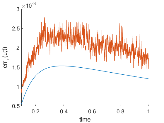
In practice it cannot be assumed that the field to be reproduced is perfectly known so we report in fig. 9 how the reproduction error is affected by errors in the monopole and dipole densities appearing in (5) and (11) when discretized with 1000 time steps and 100 points on $\partial\Omega$ .

Say $\phi^{(n)}\in\mathbb{R}^{100}$ is a vector representing the values of either the monopole or dipole density in one of the boundary representation formulas at time $n\Delta t$ , where $\Delta t$ is the time step. We perturb $\phi^{(n)}$ with a vector $\delta\phi^{(n)}\in\mathbb{R}^{100}$ with independent identically distributed zero mean Gaussian entries with standard deviation being a fraction (3%) of $\|\phi^{(n)}\|_{2}$ . For clarity we only show the error for a single realization of the perturbation $\delta\phi^{(n)}$ . The errors we observe in fig. 9 oscillate rapidly because we introduced a random perturbation at every single time step. As expected, the error we introduced in the densities increases the overall error at every single time step. We include code to generate the spatial distribution of the reconstruction errors as supplementary material (see README file), we observe that the maximum error over a time window is attained near $\partial\Omega$ as predicted by the maximum principle (remarks 2.2 and 2.8). Since the additive noise comes from perturbing the monopole and dipole densities, this perturbation is also a smooth solution of the heat equation (see section 5), which makes the maximum principle applicable.

Remark 2.9.

In the numerical results we present, the exterior errors, relative and absolute, are smaller than the interior errors. We also see a transient effect in the absolute exterior error. We believe this is similar to the temperature distribution near a point source, which also increases and then decreases with time. Since the errors that we report in figs. 7, 8 and 9 are based on the $L^{2}$ norm, the maximum principle considerations of remarks 2.2 and 2.8 do not apply directly to these numerical experiments.

3. Cloaking

The goal here is to use the results from section 2 to cloak sources or objects inside a cloaked region, by placing sources on the surface of the region. By cloaking we mean that it is hard to detect the object or source from only thermal measurements made outside the cloaked region. The boundary representation formulas of section 2 give us the appropriate surface source distribution. We start in section 3.1 with the interior cloaking of a source, directly applying the boundary representation formula in section 2.2. The interior cloaking of an object is illustrated in section 3.2 by using the boundary representation formula in section 2.1. The boundary representation formulae impose restrictions on what can be cloaked and how. In either case the field must be known for all time and with no sources in the region where it is reproduced. For the interior cloaking of a source, the temperature field generated by this source must also satisfy 2.3.

3.1. Cloaking a source in an unbounded domain

Given certain kinds of localized heat source distributions, we can find an active surface surrounding the source so that the source cannot be detected by an observer outside the surface. Let $v_{i}(x,t)$ be a free space solution to the heat equation (2) with zero initial condition and compactly supported source distribution $h(x,t)$ . Let $\Omega$ be an open bounded set (with Lipschitz boundary) that contains the support of the source $h(x,t)$ for $t>0$ . In an analogy with wave problems, we call $v_{i}$ the “incident field” and we further assume that it satisfies the growth 2.3. By theorem 2.5, we can find monopole and dipole densities on $\partial\Omega$ so that the boundary representation formula (11) gives $-v_{i}$ outside of $\overline{\Omega}$ and $0$ inside $\Omega$ . We call this the cloaking field $v_{c}$ and it is given for $t>0$ by

(31)

v_{c}(x,t)=\begin{cases}0&x\in\Omega\\ -v_{i}(x,t)&x\notin\overline{\Omega}.\end{cases}

In this manner the total field $v_{\text{tot}}=v_{i}+v_{c}$ is zero outside of $\overline{\Omega}$ and equal to $v_{i}$ inside $\Omega$ . Because the active surface $\partial\Omega$ perfectly cancels the effect of the source $h(x,t)$ for $x\notin\overline{\Omega}$ , the source cannot be detected by an observer. Figure 5 shows a numerical example of $v_{c}$ .

3.2. Cloaking passive objects in an unbounded domain

One way to detect an object in free space using only thermal measurements would be to generate an incident or probing field $u_{i}(x,t)$ with a source distribution $h(x,t)$ , i.e. a solution to the heat equation (2) in free space with zero initial condition and $h$ as its source term. In the presence of an object, the total field is given by $u_{\text{tot}}=u_{i}+u_{s}$ , where $u_{s}$ is the field “scattered” by the object, borrowing terminology from the wave equation. The scattered field is produced by the interaction between the incident field and the object and depends on the properties of the object (boundary condition, heat conductivity, $\ldots$ ). We point out that $u_{s}(x,0)=0$ because $u_{\text{tot}}(x,0)=u_{i}(x,0)$ . Having $u_{s}\neq 0$ reveals the presence of an object. In the following we assume that the object is “passive”, meaning that the scattered field is linear in the incident field. In particular this means that $u_{s}=0$ when $u_{i}=0$ . Examples of passive objects include objects with homogeneous linear boundary conditions (e.g. Dirichlet, Neumann or Robin) or objects with a heat conductivity that is different from that of the surrounding medium (see e.g. [47, 48] for transmission problems for the heat equation). We point out that the object is assumed to be open with Lipschitz boundary.

The results in section 2 can be used to cloak a passive object $R$ by placing it inside a cloaking region $\Omega$ (i.e. a bounded open set $\Omega$ with smooth boundary such that $\overline{R}\subset\Omega$ ) and makes this whole region invisible from probing incident fields $u_{i}$ generated by a source $h$ spatially supported in $\mathbb{R}^{d}-\Omega$ . Indeed, by controlling monopoles and dipoles on $\partial\Omega$ , the region $\Omega$ and the object within can be made indistinguishable from a patch of homogeneous medium, from the perspective of thermal measurements outside of $\overline{\Omega}$ . In a similar manner to section 3.1, the idea is to use (5) to cancel the incident field in $\Omega$ , while leaving the outside of $\overline{\Omega}$ unperturbed. The cloaking field, $u_{c}$ , produced by this active surface $\partial\Omega$ is then for $t>0$ :

(32)

u_{c}(x,t)=\begin{cases}-u_{i}(x,t)&x\in\Omega,\\ 0&x\notin\overline{\Omega}.\end{cases}

In principle, this cloaking field can be used to perfectly cancel the incident field in $\Omega$ for all $t>0.$ Since the temperature of the “modified incident field”: $u_{i}+u_{c}$ is zero in $\Omega$ , the temperature field surrounding the object vanishes and no scattered field is produced. In practice, the field $u_{i}+u_{c}$ in the vicinity of the object does not perfectly vanish, but we expect it to be sufficiently close to zero so that the scattered field $u_{s}$ is very small (because of linearity).

Our technique is illustrated with an object with homogeneous Dirichlet boundary conditions in fig. 10. Here the field $u_{i}$ is generated by a point source at $x=(0.9,0.3)$ and $t=0$ . For the heat equation we took $k=0.2$ and the cloaked region is $\Omega=B(x_{0},r)$ with $x_{0}=(0.5,0.5)$ and $r=1/3$ . We computed the fields on the unit square $[0,1]^{2}$ with a $200\times 200$ uniform grid. The field $u_{c}$ is found by approximating the integral (5) using the midpoint rule in time with 600 equal length subintervals of $[0,0.5]$ and the trapezoidal rule on $\partial\Omega$ with 128 uniformly spaced points. A more detailed explanation, including how the scattered fields are calculated, is in section 5. We represent in figure fig. 10 the total fields respectively generated by the incident field $u_{i}$ (left column) and by the ”modified incident field”: $u_{i}+u_{c}$ (right column). As can be seen in the right column, the temperature fields, outside of the cloaked region are indistinguishable from the incident field $u_{i}$ . We do not include a detailed error plot for this configuration, as the error is similar to the one we encountered when studying the interior reproduction problem.

Remark 3.1.

Here are two ways of dealing with active objects, i.e. that are not passive. First if the object produces a non-zero scattered field $u_{s}$ when $u_{i}=0$ , the object acts as a source and $u_{s}$ can be cancelled using the technique in section 3.1. This presumes perfect knowledge of $u_{s}$ and $u_{i}$ . Second, if the object does not produce a scattered field when immersed in some harmonic field $u_{0}$ , we can use as a cloaking field $u_{c}(x,t)=-u_{i}(x,t)+u_{0}(x)$ for $x\in\Omega$ and $u_{c}(x,t)=0$ for $x\notin\overline{\Omega}$ , instead of (32). An example of such an object would be one with a constant $c\neq 0$ Dirichlet boundary condition. By our assumption, the field $u_{0}(x)=c$ does not create any scattering, regardless of the shape of the object.

4. Mimicking

Another possible application of the boundary representation formulas (5) and (11) is to mimic sources or passive objects. This is done in two steps. First we cancel out the original source or suppress the scattering of the original object using a source distribution on a surface $\partial\Omega$ surrounding the object. Second we adjust the source distribution so that the object or source appears to the observer as another object or source. We illustrate this idea with two cases: making sources look like other sources (section 4.1) and making a passive object look like a different passive object (section 4.2). Other combinations are possible but are not presented here.

4.1. Source mimicking

For source mimicking, we consider the problem where there is a compactly supported source distribution, $f(x,t)$ which we seek to make appear as a different compactly supported source distribution, $g(x,t)$ from thermal measurements outside of a region $\overline{\Omega}$ (where $\Omega$ is an open bounded set with Lipschitz boundary). The support of both distributions is assumed to be contained in $\overline{\Omega}$ for all $t>0$ . The two corresponding solutions to the heat equation (2) are $v(x,t;f)$ and $v(x,t;g)$ , and we further assume they satisfy 2.3.

Mimicking can be achieved by simultaneously canceling the field $v(x,t;f)$ outside $\overline{\Omega}$ and adding $v(x,t;g)$ also outside $\overline{\Omega}$ . Both can be done using the results in section 3.1. That is, using (31) we can find a monopole and dipole density on $\partial\Omega$ that generates a field

(33)

v_{c}(x,t)=\begin{cases}0&x\in\Omega,\\ v(x,t;g)-v(x,t;f)&x\notin\overline{\Omega}.\end{cases}

In this way the field $v(x,t;f)+v_{c}(x,t)$ is equal to $v(x,t;g)$ outside of $\overline{\Omega}$ , as desired.

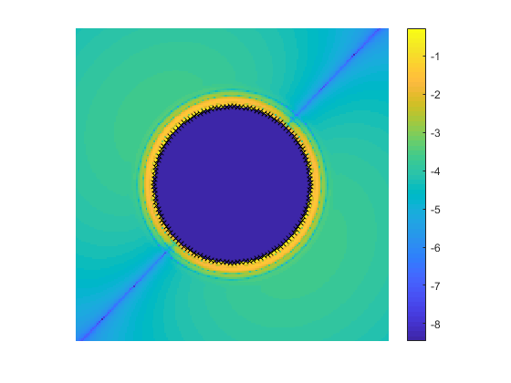
A numerical example to illustrate the method is given in fig. 11. Fields are calculated in $[0,1]^{2}$ using a uniform grid of 200 by 200 points at $t=0.2$ s. Here a point source at $y^{(1)}=(0.6,0.4)$ and $t=0$ is made to appear as a point source at $y^{(2)}=(0.39,0.6)$ and $t=0$ , from thermal measurements outside of $\overline{\Omega}$ . Figure 11 (a) and (b) represent the fields $v(x,t;f)$ and $v(x,t;g)$ , where $f(x,t)=\delta(x-y^{(1)},t)$ and $g(x,t)=\delta(x-y^{(2)},t)$ . Figure 11(c) shows the field $v(x,t;f)+v_{c}(x,t)$ , where $v_{c}$ has been constructed by applying (33). An error plot is shown in fig. 11(d) where the error is largest near the boundary as we expect based on the sensitivity analysis of section 2. We believe the diagonal line with small error in fig. 11(d) is an artifact of our choice of sources.

4.2. Mimicking a passive object

Consider a passive object $R$ that is completely contained in an open set $\Omega$ and a source exterior to $\Omega$ which produces the incident field $u_{i}$ . The goal is to make $R$ look like a different passive object, $S$ , from thermal measurements outside $\overline{\Omega}$ . To achieve this we can use linearity and both the interior and exterior boundary representation formulas to find monopole and dipole densities on $\partial\Omega$ producing a field

(34)

u_{c}(x,t)=\begin{cases}-u_{i}(x,t),&x\in\Omega,\\ v_{s}(x,t),&x\notin\overline{\Omega},\end{cases}

where $v_{s}(x,t)$ is the scattered field corresponding to the object $S$ , included also in $\Omega$ , resulting from the incident field $u_{i}(x,t)$ . In this fashion the total field is $u_{i}(x,t)+v_{s}(x,t)$ outside of $\overline{\Omega}$ and $0$ inside of $\Omega$ . Its associated scattered field is $v_{s}(x,t)$ outside of $\overline{\Omega}$ and $0$ inside of $\Omega-{R}$ as desired.

To illustrate the method we consider a “kite” object with homogeneous Dirichlet boundary conditions and make it appear as a “flower” object with identical boundary conditions. Here the field $u_{i}$ is generated by a point source at $x=(0.25,0.5)$ and $t=0$ . For the heat equation we took $k=0.2$ and the domain is $\Omega=B(x_{0},r)$ with $x_{0}=(0.5,0.5)$ and $r=0.25$ . We computed the fields on the unit square $[0,1]^{2}$ with a $200\times 200$ uniform grid. The field $u_{c}$ is found by approximating the integral (5) using the midpoint rule in time with 180 equal length subintervals of $[0,0.05]$ and the trapezoidal rule on $\partial\Omega$ with 128 uniformly spaced points. A more detailed explanation, including how the scattered fields are calculated, is in section 5. Figure 12(a) and (b) show the scattered fields from two different objects and fig. 12(c) shows the mimicked scattered field. Because we are approximating the fields numerically, the field $u_{i}+u_{c}$ is very close to zero in $\Omega$ , but not exactly zero. The errors (which are not reported here) are larger near the boundary and decay as we move outwards, as we observed in section 2.

Remark 4.1.

Although we have only shown mimicking of passive objects, the same techniques outlined in remark 3.1, could be used to suppress the field generated by an active object, which is part of what needs to be done to mimic an active object.

5. A simple numerical approach to potential theory for the heat equation

The boundary representation formulas (5) and (11) can expressed very efficiently in terms of the single and double layer potentials for the heat equation defined for $t>0$ by

	$\displaystyle\mathcal{K}_{0}(\psi)(x,t)$	$\displaystyle=\int_{0}^{t}ds\int_{\partial\Omega}dS(y)[\psi(y,s)K(x-y,t-s)],\;x\notin\partial\Omega,$
	$\displaystyle\mathcal{K}_{1}(\varphi)(x,t)$	$\displaystyle=\int_{0}^{t}ds\int_{\partial\Omega}dS(y)[\varphi(y,s)\frac{\partial K}{\partial n}(x-y,t-s)],\;x\notin\partial\Omega,$

as well as the corresponding boundary layer operators given for $t>0$ by

	$\displaystyle\mathcal{V}(\psi)(x,t)$	$\displaystyle=\int_{0}^{t}ds\int_{\partial\Omega}dS(y)[\psi(y,s)K(x-y,t-s)],\;x\in\partial\Omega,$
	$\displaystyle\mathcal{K}(\varphi)(x,t)$	$\displaystyle=\int_{0}^{t}ds\int_{\partial\Omega}dS(y)[\varphi(y,s)\frac{\partial K}{\partial n}(x-y,t-s)]\;x\in\partial\Omega,$

where $\phi(x,t)$ and $\psi(x,t)$ are time dependent densities defined on $\partial\Omega$ . A full derivation of these and other potential theory operators for the heat equation and their properties can be found in [34, 39, 49]. For a review of classic potential theory see e.g. [50, 45, 39, 51].

With the potential theory notation, the interior boundary representation formula (5), with zero initial condition, becomes

(35)

u_{\Omega}(x,t)=\mathcal{K}_{0}\Big(\frac{\partial u}{\partial n}\Big)(x,t)-\mathcal{K}_{1}(u)(x,t).

Whereas the exterior boundary representation formula (11) becomes

(36)

v_{\Omega}(x,t)=\mathcal{K}_{1}(v)(x,t)-\mathcal{K}_{0}\Big(\frac{\partial v}{\partial n}\Big)(x,t).

Galerkin methods are commonly used to approximate the spatial integrals in eqs. 36 and 35, with a number of different approaches to deal with the integration in time. For instance time marching [33], time-space Galerkin methods [42, 44] convolution quadrature [43] and collocation [52]. For simplicity we opted for an approach based on the trapezoidal rule for the integration on $\partial\Omega$ and the midpoint rule for the time convolution. To be more precise, there are two convolutions that need to be evaluated in order to calculate the boundary representations in (35) and (36); a convolution in space and a convolution in time. For the spatial integration, trapezoidal rule is used with uniformly placed points on a parametric representation of $\partial\Omega$ . Since this amounts to integrating a periodic function, we can expect that the convergence rate of the trapezoidal rule depends explicitly on the rate of decay of the Fourier coefficients of the function to be integrated [53]. Due to the smoothness of the heat kernel, exponential convergence is expected. For the integration in time, the convolutions are of the form

\int_{0}^{t}ds\;g(s)f(t-s).

These convolutions are approximated with the midpoint rule as follows

(37)

\int_{0}^{j\Delta t}ds\;g(s)f(j\Delta t-s)\approx\Delta t\sum_{k=1}^{j}g((k-\frac{1}{2})\Delta t)f((j-k)\Delta t+\frac{1}{2}\Delta t),

which avoids evaluating $f$ at $t=0$ . This is handy in our case because of the singularity of the heat kernel at $(x,t)=(0,0)$ , which only occurs for boundary layer operators. After this space-time discretization, the resulting approximations are by construction an interpolation on the space-time grid of a finite distribution of monopoles and dipoles located on $\partial\Omega$ . These distributions are smooth solutions of the homogeneous heat equation on any open set of $(\mathbb{R}^{d}-\partial\Omega)\times\mathbb{R}$ . Moreover lemma 2.7 (see eq. (25)) ensures that they are bounded for $t>0$ and $x\notin B(0,r)$ for $r$ large enough. Thus, as they satisfy eq. 28, we can apply the maximum principle over any finite time window $[t_{1},t_{2}]$ (with $0\leq t_{1}<t_{2}$ ) on any closed set of $\mathbb{R}^{d}-\overline{\Omega}$ that does not intersect $\partial\Omega$ . We leave an accuracy study of the numerical approximation we use to future work. In particular there are more accurate ways of dealing with the approximation for $s\in[0,\Delta t]$ than the midpoint rule we use, see e.g. [33, 42, 52, 54].

5.1. Scattered field computation

In the case of inclusions, finding the scattered field requires the use of the boundary layer operators. For simplicity we only consider a homogeneous Dirichlet inclusion, $R$ , i.e. where the temperature on $\partial R$ is held constant at $0$ . Neumann inclusions, and inclusions with varying thermal diffusivity, require the introduction of other boundary integral operators (adjoint double layer and hypersingular [34]), but a similar numerical approach can be applied to this case.

The idea is to look for a scattered field $u_{s}$ of the form (36) outside of $R$ . Since the temperature at $\partial R$ is constant and equal to $0$ , the scattered field satisfies $u_{s}|_{\partial R}=-u_{i}|_{\partial R}$ . Hence we know the Dirichlet data on $\partial R$ in the representation formula (36), but not the Neumann data. We treat this as an unknown boundary density $\psi$ in

(38)

u_{s}(x,t)=\mathcal{K}_{1}(-u_{i}|_{\partial R})(x,t)-\mathcal{K}_{0}(\psi)(x,t).

The latter formula is only valid for $x\notin\overline{R}$ . To obtain an integral equation on $\partial R$ we take the limit of (38) as $x$ approaches $\partial R$ . The limit could be different if we approach $\partial R$ from the inside or from the outside. The limits are given by the so-called jump relations. For $x\in\partial R$ , the jump relation needed for the single layer potential is

(39)

\lim_{z\rightarrow x}\mathcal{K}_{0}\psi(z,t)=\mathcal{V}\psi(x,t),

which holds for $z$ tending towards $\partial R$ from both the interior and exterior of $R$ . The jump relations needed for the double layer potential are

(40)

\lim_{z\rightarrow x^{+}}\mathcal{K}_{1}\varphi(z,t)=\frac{1}{2}\varphi(x,t)+\mathcal{K}\varphi(x,t),~\text{and}\lim_{z\rightarrow x^{-}}\mathcal{K}_{1}\varphi(z,t)=\frac{-1}{2}\varphi(x,t)+\mathcal{K}\varphi(x,t),

where $z\to x^{+}$ denotes approaching $\partial R$ from the exterior of $R$ and $z\to x^{-}$ from the interior. Using these jump relations and (38) we have

(41)		$\displaystyle\lim_{z\rightarrow x^{+}}u_{s}(z,t)$	$\displaystyle=\lim_{z\rightarrow x^{+}}\mathcal{K}_{1}(-u_{i}(z,t))-\lim_{z\rightarrow x^{+}}\mathcal{K}_{0}\psi(z,t)$
(41)		$\displaystyle\Rightarrow-u_{i}\|_{\partial R}$	$\displaystyle=\frac{-1}{2}u_{i}\|_{\partial R}+\mathcal{K}(-u_{i}\|_{\partial R})-\mathcal{V}\psi.$

Rearranging terms yields a boundary integral equation for $\psi$

(42)

\mathcal{V}\psi=\frac{u_{i}|_{\partial R}}{2}+\mathcal{K}(-u_{i}|_{\partial R}).

We discretize (42) as a linear system where the unknown is $\psi$ evaluated on a uniform grid of $\partial R$ and of $[0,T]$ . The boundary integral operators $\mathcal{V}$ and $\mathcal{K}$ in (42) are discretized using the trapezoidal rule in space and the midpoint rule in time. For instance, $\mathcal{V}$ is approximated by a $MN\times MN$ matrix which is lower triangular by blocks, with each block of size $N\times N$ . Here $M$ is the number of time steps and $\partial R$ is approximated by a polygon with $N$ sides:

(43)

\mathcal{V}\approx\left[\begin{array}[]{cccc}V_{\frac{1}{2}}&&&\\[11.99998pt] V_{\frac{3}{2}}&V_{\frac{1}{2}}&&\\ \vdots&&\ddots&\\ V_{M-\frac{1}{2}}&V_{M-\frac{3}{2}}&\cdots&V_{\frac{1}{2}}\end{array}\right].

The $V_{i}$ are $N\times N$ matrices with entries $(V_{i})_{jk}=\ell_{k}K(x_{j}-x_{k},i\Delta t)$ , where $x_{k}$ is the center of the $k-$ th segment of length $\ell_{k}$ . Clearly the matrix in (43) is guaranteed to be invertible if $V_{\frac{1}{2}}$ is invertible. Though we have not studied the invertibility of $V_{\frac{1}{2}}$ , we observe that it may become singular for a given spatial discretization if the temporal discretization is not fine enough.

6. Summary and perspectives

We proposed a strategy for active cloaking for the time-dependent parabolic heat (or mass, or diffusive light) equation. Similar to previous work for active cloaking for e.g. the Helmholtz or Laplace equation (e.g. modelling time-harmonic waves and thermostatic problems), our results rely on active sources coming from Green identities to reproduce solutions inside or outside a bounded domain. The idea is to use a source distribution on a closed surface to reproduce certain solutions to the heat equation inside the surface and the zero solution outside or vice versa. We give a growth condition which is sufficient to guarantee that a solution to the heat equation can be reproduced outside of a closed surface. We apply these theoretical results in four ways: interior cloaking of a source, interior cloaking of an object, source mimicking, and object mimicking. For the cloaking problems the idea is to find an active surface that surrounds the object or source to make the object or source undetectable by thermal measurements outside the surface. In the mimicking problems, instead of making the object undetectable, we make the source or object appear as a different source or object from the perspective of thermal measurements outside the cloak. Our solution to these problems inherits the limitations of the reproduction method, namely that the fields must be known for all time on the active surface surrounding the object or source we want to cloak or mimic. However the maximum principle guarantees some stability of our approach, as it is based on boundary representation formulas. This is a special feature of the heat equation. We illustrate our method with simple potential theory based simulations which are consistent with the heat equation and thus allow us to interpret the numerical errors using the maximum principle. Our study was limited to the case where the initial condition is zero or harmonic. It may be possible to use (6) to cancel out the initial condition with a boundary integral, but (a) it is not clear whether this mathematical construct has a physical interpretation and (b) this representation formula is only valid inside a bounded domain. These are questions we plan on exploring. Although we focused on the isotropic heat equation, it may be possible to carry out a similar cloaking strategy for anisotropic media and when an advection term is added to the heat equation. Our approach could also be tied to the active cloaking strategies for the Helmholtz equation in [18, 17] by going to Fourier or Laplace domain in time, so that the active sources do not completely surround the object to achieve partial cloaking. For the Fourier domain, the physical interpretation is to study time-harmonic sources. Another open question is whether the growth condition we provided is optimal and how it is related to the uniqueness question for the exterior problem associated with different boundary condition types for the heat equation.

We note that this work could be also adapted to cloaking [55, 56] and mimicking [57] of quantum matter waves. We believe this approach could be further generalized to the Fokker-Plank equation arising in statistical mechanics, which could applied to gravitational systems for which some passive cloaking theory has been proposed [58]. Finally, as some scattering cancellation based cloaking approach has been proposed for Maxwell-Cataneo heat waves [59], we believe that our method for active cloaking could be also applied to such pseudo-waves.

Data Access. The Matlab code to reproduce the figures figs. 3, 5, 7, 8, 9, 10, 11 and 12 is available in repository [TBA]. For example, fig. 3 can be reproduced by running the Matlab script fig3.m. The scripts for figs. 3 and 5 generate additional plots that are mentioned in the respective figure captions. Figure 10 is animated in movie1.mp4. The spatial distribution for the monopole/dipole added noise (section 2.3) can be generated with the scripts fig9supint.m and fig9supext.m.

Author Contributions. SG suggested the problem and applications to other physical phenomena. MC, TD, and FGV proved the exterior representation formula and the other theoretical results. All authors designed the numerical experiments. TD and FGV performed the numerical experiments. All authors contributed to the writing.

Funding. TD and FGV were supported by National Science Foundation Grant DMS-2008610.

Acknowledgemnts. FGV acknowledges support from the Fresnel institute for a visit in January 2018 during which the idea for this article first came up. FGV also thanks the Jean Kuntzmann Laboratory for hosting the author during the 2017-2018 academic year. Last but not least, the authors acknowledge Graeme Milton for the exterior cloaking idea that inspired this work.

References

[1] Nguyen DM, Xu H, Zhang Y, Zhang B. 2015 Active thermal cloak. Applied Physics Letters 107, 121901.
[2] DiSalvo FJ. 1999 Thermoelectric Cooling and Power Generation. Science 285, 703–706.
[3] Xu L, Yang S, Huang J. 2019 Dipole-assisted thermotics: Experimental demonstration of dipole-driven thermal invisibility. Phys. Rev. E 100, 062108.
[4] Peralta I, Fachinotti V, Álvarez Hostos J. 2019 A Brief Review on Thermal Metamaterials for Cloaking and Heat Flux Manipulation. Advanced Engineering Materials 22, 1901034.
[5] Guenneau S, Puvirajesinghe TM. 2013 Fick’s second law transformed: one path to cloaking in mass diffusion. Journal of The Royal Society Interface 10, 20130106.
[6] Puvirajesinghe TM, Zhi ZL, Craster R, Guenneau S. 2018 Tailoring drug release rates in hydrogel-based therapeutic delivery applications using graphene oxide. Journal of The Royal Society Interface 15, 20170949.
[7] Zeng L, Song R. 2013 Controlling chloride ions diffusion in concrete. Scientific Reports 3, 3359.
[8] Schittny R, Kadic M, Buckmann T, Wegener M. 2014 Invisibility cloaking in a diffusive light scattering medium. Science 345, 427–429.
[9] Guenneau S, Amra C, Veynante D. 2012 Transformation thermodynamics: cloaking and concentrating heat flux. Opt. Express 20, 8207–8218.
[10] Ma Y, Lan L, Jiang W, Sun F, He S. 2013 A transient thermal cloak experimentally realized through a rescaled diffusion equation with anisotropic thermal diffusivity. NPG Asia Materials 5, e73–e73.
[11] Craster RV, Guenneau SRL, Hutridurga HR, Pavliotis GA. 2018 Cloaking via mapping for the heat equation. Multiscale Model. Simul. 16, 1146–1174.
[12] Schittny R, Kadic M, Guenneau S, Wegener M. 2013 Experiments on Transformation Thermodynamics: Molding the Flow of Heat. Phys. Rev. Lett. 110, 195901.
[13] Petiteau D, Guenneau S, Bellieud M, Zerrad M, Amra C. 2015 Spectral effectiveness of engineered thermal cloaks in the frequency regime. Scientific reports 4, 7386.
[14] Miller DAB. 2006 On perfect cloaking. Opt. Express 14, 12457–12466.
[15] Ffowcs Williams JE. 1984 Review Lecture: Anti-Sound. Proc. R. Soc. A 395, 63–88.
[16] Nelson P, Elliot SJ. 1991 Active Control of Sounds. Academic Press, New York first edition.
[17] Guevara Vasquez F, Milton GW, Onofrei D. 2009a Broadband exterior cloaking. Opt. Express 17, 14800–14805.
[18] Guevara Vasquez F, Milton GW, Onofrei D. 2009b Active Exterior Cloaking for the 2D Laplace and Helmholtz Equations. Phys. Rev. Lett. 103, 073901.
[19] Guevara Vasquez F, Milton GW, Onofrei D. 2011 Exterior cloaking with active sources in two dimensional acoustics. Wave Motion 48, 515–524. Special Issue on Cloaking of Wave Motion.
[20] Norris AN, Amirkulova FA, Parnell WJ. 2012 Source amplitudes for active exterior cloaking. Inverse Problems 28, 105002.
[21] Guevara Vasquez F, Milton GW, Onofrei D. 2012 Mathematical analysis of the two dimensional active exterior cloaking in the quasistatic regime. Analysis and Mathematical Physics 2, 231–246.
[22] Guevara Vasquez F, Milton GW, Onofrei D, Seppecher P. 2013 Transformation elastodynamics and active exterior cloaking. In Craster RV, Guenneau S, editors, Acoustic metamaterials: Negative refraction, imaging, lensing and cloaking. Springer.
[23] Norris AN, Amirkulova FA, Parnell WJ. 2014 Active elastodynamic cloaking. Math. Mech. Solids 19, 603–625.
[24] O’Neill J, Selsil O, McPhedran RC, Movchan AB, Movchan NV. 2015 Active cloaking of inclusions for flexural waves in thin elastic plates. Quart. J. Mech. Appl. Math. 68, 263–288.
[25] O’Neill J, Selsil O, McPhedran RC, Movchan AB, Movchan NV, Henderson Moggach C. 2016 Active cloaking of resonant coated inclusions for waves in membranes and Kirchhoff plates. Quart. J. Mech. Appl. Math. 69, 115–159.
[26] Avanzini F, Falasco G, Esposito M. 2020 Chemical cloaking. Phys. Rev. E 101, 060102.
[27] Ma Q, Mei ZL, Zhu SK, Jin TY, Cui TJ. 2013 Experiments on Active Cloaking and Illusion for Laplace Equation. Phys. Rev. Lett. 111, 173901.
[28] Ma Q, Yang F, Jin TY, Mei ZL, Cui TJ. 2016 Open active cloaking and illusion devices for the Laplace equation. Journal of Optics 18, 044004.
[29] Selvanayagam M, Eleftheriades GV. 2013 Experimental Demonstration of Active Electromagnetic Cloaking. Phys. Rev. X 3, 041011.
[30] Lai Y, Ng J, Chen H, Han D, Xiao J, Zhang ZQ, Chan CT. 2009 Illusion Optics: The Optical Transformation of an Object into Another Object. Phys. Rev. Lett. 102, 253902.
[31] Zheng HH, Xiao JJ, Lai Y, Chan CT. 2010 Exterior optical cloaking and illusions by using active sources: A boundary element perspective. Phys. Rev. B 81, 195116.
[32] Lions JL, Magenes E. 1973 Non-homogenous Boundary Values Problem and Applications vol. III. Springer-Verlag.
[33] Pina HLG, Fernandes JLM. 1984 Applications in transient heat conduction. In Topics in boundary element research, Vol. 1 pp. 41–58. Springer, Berlin.
[34] Costabel M. 1990 Boundary integral operators for the heat equation. Integral Equations Operator Theory 13, 498–552.
[35] Friedman A. 1964 Partial differential equations of parabolic type. Prentice-Hall, Inc., Englewood Cliffs, N.J.
[36] DLMF NIST Digital Library of Mathematical Functions. http://dlmf.nist.gov/, Release 1.0.21 of 2018-12-15. F. W. J. Olver, A. B. Olde Daalhuis, D. W. Lozier, B. I. Schneider, R. F. Boisvert, C. W. Clark, B. R. Miller and B. V. Saunders, eds.
[37] Brezis H. 2011 Functional analysis, Sobolev spaces and partial differential equations. Springer.
[38] Evans LC. 2010 Partial differential equations vol. 19, Graduate Studies in Mathematics. American Mathematical Society second edition.
[39] Kress R. 2014 Linear integral equations. vol. 82, Applied Mathematical Sciences. Springer third edition.
[40] Tychonoff A. 1935 Théorèmes d’unicité pour l’équation de la chaleur. Mat. Sb. 42, 199–216.
[41] Arnold DN, Noon PJ. 1987 Boundary integral equations of the first kind for the heat equation. In Boundary elements IX, Vol. 3 (Stuttgart, 1987) pp. 213–229. Comput. Mech., Southampton.
[42] Noon PJ. 1988 The single layer heat potential and Galerkin boundary element methods for the heat equation. PhD thesis. Thesis (Ph.D.)–University of Maryland, College Park.
[43] Qiu T, Rieder A, Sayas FJ, Zhang S. 2019 Time-domain boundary integral equation modeling of heat transmission problems. Numer. Math. 143, 223–259.
[44] Dohr S. 2019 Distributed and Preconditioned Space–Time Boundary Element Methods for the Heat Equation. PhD thesis Graz University of Technology.
[45] Colton D, Kress R. 2013 Inverse acoustic and electromagnetic scattering theory vol. 93, Applied Mathematical Sciences. Springer, New York third edition.
[46] Lions JL, Magenes E. 1972 Non-homogenous Boundary Values Problem and Applications vol. II. Springer-Verlag.
[47] Ammari H, Iakovleva E, Kang H, Kim K. 2005 Direct Algorithms for Thermal Imaging of Small Inclusions. Multiscale Model. Simul. 4, 1116–1136.
[48] Hohage T, Sayas F. 2005 Numerical solution of a heat diffusion problem by boundary element methods using the Laplace transform. Numerische Mathematik 102, 67–92.
[49] Costabel M, Sayas F. 2017 Time‐dependent problems with the boundary integral equation method. Encyclopedia of Computational Mechanics Second Edition pp. 1–24.
[50] Costabel M. 1988 Boundary integral operators on Lipschitz domains: elementary results. SIAM J. Math. Anal. 19, 613–626.
[51] Ammari H, Kang H, Lee H. 2009 Layer potential techniques in spectral analysis vol. 153Mathematical Surveys and Monographs. American Mathematical Society, Providence, RI.
[52] Martti H, Saranen J. 1994 On the spline collocation method for the single-layer heat operator equation. Mathematics of Computation 62, 41–64.
[53] Hyde EM. 2003 Fast, high-order methods for scattering by inhomogeneous media. ProQuest LLC, Ann Arbor, MI. Thesis (Ph.D.)–California Institute of Technology.
[54] Tausch J. 2007 A fast method for solving the heat equation by layer potentials. J. Comput. Phys. 224, 956–969.
[55] Zhang S, Genov D, Sun C, Zhang X. 2008 Cloaking of matter waves. Phys. Rev. Lett. 100, 123002.
[56] Greenleaf A, Kurylev Y, Lassas M, Uhlmann G. 2008 Isotropic transformation optics: approximate acoustic and quantum cloaking. New J. Phys. 10, 115024.
[57] Diatta A, Guenneau S. 2010 Non-singular cloaks allow mimesis. Journal of Optics 13, 024012.
[58] Smerlak M. 2012 Diffusion in curved spacetimes. New J. Phys. 14, 023019.
[59] Farhat M, Guenneau S, Chen P, Alu A, Salama K. 2019 Scattering cancellation-based cloaking for the Maxwell-Cattaneo heat waves. Physical Review Applied 11, 044089.

(17)	$\displaystyle\int_{0}^{t}ds[s^{-d/2}e^{-\|x-r\xi\|^{2}/4ks}]$	$\displaystyle=\int_{+\infty}^{\|x-r\xi\|^{2}/4kt}du\left[{\frac{(4ku)^{d/2}}{\|x-r\xi\|^{d}}\left(\frac{-\|x-r\xi\|^{2}}{4ku^{2}}\right)e^{-u}}\right]$
		$\displaystyle=\frac{(4k)^{d/2-1}}{\|x-r\xi\|^{d-2}}\int^{+\infty}_{\|x-r\xi\|^{2}/4kt}du[u^{d/2-1-1}e^{-u}]$
		$\displaystyle=\frac{(4k)^{d/2-1}}{\|x-r\xi\|^{d-2}}\Gamma\bigg(\frac{d}{2}-1,\frac{\|x-r\xi\|^{2}}{4kt}\bigg),$


(a) Uncloaked object at $t=.05$ s	(b) Cloaked object at $t=.05$ s

(c) Uncloaked object at $t=.25$ s	(d) Cloaked object at $t=.25$ s

(e) Uncloaked object at $t=.5$ s	(f) Cloaked object at $t=.5$ s


(a) Original source	(b) Source to mimic

(c) Mimicked source	(d) $\log_{10}$ plot of errors


(a) Original field	(b) Reconstructed field	(c) $\log_{10}$ plot of errors


(a) Original field	(b) Reproduced field	(c) $\log_{10}$ plot of errors

	interior error	exterior error
Interior reproduction problem
Exterior reproduction problem


(a) Scattered field from a kite	(b) Scattered field from a flower	(c) Mimicked scattered field