Can cosmological simulations capture the diverse satellite populations of observed Milky Way analogues?2020Can cosmological simulations capture the diverse satellite populations of observed Milky Way analogues?–16
Abstract
The recent advent of deep observational surveys of local Milky Way ‘analogues’ and their satellite populations allows us to place the Milky Way in a broader cosmological context and to test models of galaxy formation on small scales. In the present study, we use the CDM-based ARTEMIS suite of cosmological hydrodynamical simulations containing 45 Milky Way analogue host haloes to make comparisons to the observed satellite luminosity functions, radial distribution functions, and abundance scaling relations from the recent Local Volume and SAGA observational surveys, in addition to the Milky Way and M31. We find that, contrary to some previous claims, CDM-based simulations can successfully and simultaneously capture the mean trends and the diversity in both the observed luminosity and radial distribution functions of Milky Way analogues once important observational selection criteria are factored in. Furthermore, we show that, at fixed halo mass, the concentration of the simulated satellite radial distribution is partly set by that of the underlying smooth dark matter halo, although stochasticity due to the finite number of satellites is the dominant driver of scatter in the radial distribution of satellites at fixed halo mass.
Keywords:
Local Group, galaxies: luminosity function, galaxies: dwarf, galaxies: formation, galaxies: evolution1 Introduction
The formation of the Milky Way has traditionally been considered as a blueprint for understanding the formation of normal spiral galaxies in general. The adoption of this assumption has perhaps been mainly motivated by the fact that, typically, there has been much higher quality and detailed observations available for the Milky Way than for any other galaxy. To what extent the Milky Way is actually representative of disc galaxies is presently uncertain, though. With the advent of new deep, dedicated extragalactic surveys of so-called “Milky Way analogues” (i.e., disc galaxies with total halo masses of ) in the Local Volume (Danieli et al. 2017; Smercina et al. 2018; Bennet et al. 2019; Crnojević et al. 2019; Bennet et al. 2020; Carlsten et al. 2020a) and out to Mpc (Geha et al. 2017; Mao et al. 2021), there is a rapidly diminishing requirement to rely on the Milky Way as our template for disc galaxy formation. Instead, the rapid increase in the number of Milky Way-mass galaxies with high-quality data available, both in observations and in cosmological simulations, motivates a reassessment of what constitutes a typical disc galaxy and how the Milky Way fits into this picture.
Work along these lines has suggested that the Milky Way may not have had a typical merger history for a galaxy of total mass of . In particular, the Milky Way appears to have had a very quiescent history since (e.g., Wyse 2001; Deason et al. 2013; Ruchti et al. 2015; Lancaster et al. 2019), which is relatively rare in a cosmological context (e.g., Stewart et al. 2008; Font et al. 2017). In contrast, M31, another well-studied disc galaxy of similar mass to our own, shows evidence of a much more active accretion history, as indicated by its disturbed stellar disc, ubiquitous tidal debris in its stellar halo and a significantly higher abundance of satellite galaxies (e.g. McConnachie et al. 2009; McConnachie et al. 2018; Deason et al. 2013; D’Souza & Bell 2018). As galaxies and their dark matter haloes in CDM are, to a large extent, assembled through the accretion and mergers of smaller satellite galaxies, the properties of the satellite population (e.g., its abundance, spatial distribution, internal properties) contain a significant amount of information about the formation histories of their hosts. They are effectively proxies for the formation histories of galaxies and by examining the satellite populations11 1 A caveat, of course, is that some satellites are completely disrupted and/or merged with the central galaxy, implying that the current satellite population does not contain a complete census of merger history of the system. But this information is ultimately retained in the properties of the stellar halo and the central galaxy and is therefore potentially recoverable. of hosts of (approximately) fixed mass, we are effectively examining the differing formation histories that lead to galaxies of a fixed mass.
Advances in observational surveys have resulted in growing samples of dwarf satellite galaxies around dozens of Milky Way analogues. Given the distances to these galaxies, the samples are complete only in the ‘classical’ dwarf regime (e.g. limiting magnitudes of or for galaxies in the Local Volume or to out to Mpc). Nevertheless, the properties of Local Group classical dwarf galaxies can now be put into a broader ‘cosmological’ context.
Apart from the question of Milky Way’s typicality, there is also the question of whether theoretical models (specifically, whether cosmological simulations based on a CDM cosmology) can generally reproduce the properties of observed satellite galaxies. The current cosmological model has been confronted with several ‘small-scale problems’, including: the so-called missing satellite problem (e.g., Kauffmann et al. 1993; Klypin et al. 1999; Moore et al. 1999), the ‘too big to fail’ problem (Read et al. 2006; Boylan-Kolchin et al. 2011; Boylan-Kolchin et al. 2012), and the cusp-core problem (Flores & Primack 1994; Moore 1994). These apparent problems are present in both the Milky Way and M31 (Tollerud et al. 2014). A variety of potential solutions to these problems have been proposed (both within the context of CDM and beyond), starting with observational bias corrections (Koposov et al. 2008; Tollerud et al. 2008; Koposov et al. 2009; Jethwa et al. 2018; Kim et al. 2018, e.g.) and invoking baryonic processes (Governato et al. 2012; Pontzen & Governato 2012; Brooks & Zolotov 2014; Sawala et al. 2016; Wetzel et al. 2016), changing the nature of dark matter, such as warm or self-interacting dark matter (Spergel & Steinhardt 2000; Rocha et al. 2013; Lovell et al. 2014), changing the nature of gravity (e.g., Brada & Milgrom 2000), or the values of some of the cosmological parameters that preferentially affect small scales, such as the running of the scalar spectral index of primordial fluctuations (Garrison-Kimmel et al. 2014; Stafford et al. 2020). In the present study it is not our aim to re-examine these well-studied questions.
The observations of Milky Way analogues and of their satellite populations provide a renewed motivation to test the predictions of cosmological models. Although most of the small-scale problems above require resolved stellar spectroscopy, which is not currently possible beyond the Local Group, observations of distant Milky Way analogues provide other useful small-scale tests. In addition to determining the satellite luminosity functions, they also provide measurements of the largest magnitude gaps in these functions (which can give an indication of their slopes) and of the spatial distributions of dwarf galaxies. With a growing sample of Milky Way-mass galaxies, these observables can in principle be correlated with the properties of host galaxies. Additionally, the system-to-system scatter in the observables (e.g., luminosity functions and radial distributions) can be quantified and compared with theoretical predictions. Needless to say, a successful theory should not only capture the mean trends but also the scatter about them.
Observations of Milky Way analogues to date have already revealed some new and interesting puzzles about the populations of classical dwarfs. These include:
- •
Too large scatter in the luminosity functions? Some disc galaxies display a strikingly low number of bright satellites compared with the Milky Way. For example, M94, dubbed as the ‘lonely giant’ (Smercina et al. 2018) has only two satellites brighter than within kpc. Another large disc galaxy, M101, has only satellites brighter than within the same radius (Danieli et al. 2017; Bennet et al. 2019; Bennet et al. 2020). For comparison, the median number of classical dwarf satellites per host in the Local Volume is (Bennet et al. 2019), a number that is similar to that found for M31 (McConnachie 2012). Cosmological hydrodynamical simulations that contain a statistical sample of Milky Way-mass galaxies with their satellite populations can potentially elucidate whether sparse systems such as M94 or M101 occur naturally in a CDM model.
- •
Tensions between the observed and predicted radial distributions of satellites. The radial distribution of Milky Way satellites appears to stand in contrast with the predictions of CDM models, in the sense that it appears to be more centrally-concentrated than typical simulated Milky Way-mass systems (Kravtsov et al. 2004; Yniguez et al. 2014; Samuel et al. 2020). Previous studies have shown that the incorporation of important baryonic physics can help to reconcile this tension (e.g., Kravtsov et al. 2004; Macciò et al. 2010; Font et al. 2011; Starkenburg et al. 2013). Alternatively, or in addition to, it is possible that simulations with limited numerical resolution may suffer from the spurious tidal disruption of satellites (e.g., van den Bosch & Ogiya 2018) or that an overly energetic feedback results in satellites being centrally cored and therefore more vulnerable to disruption. Another possibility is that the discrepant radial distributions may be reconciled if the observed tally of dwarf galaxies beyond kpc from the centre of the Milky Way is incomplete (Garrison-Kimmel et al. 2019). As we will discuss in this paper, we find an inverse radial distribution problem, where dwarf galaxies around some Milky Way analogues in the SAGA survey (Mao et al. 2021) appear, at face value, to be significantly less centrally-concentrated than predicted. Therefore, careful comparisons between models and observations are required in order to understand the causes of these apparently contradictory results.
- •
As already noted, a number of possible scaling relations between the abundance of surviving satellites and the properties of their hosts galaxies have been examined, including correlations with the host total mass (Trentham & Tully 2009; Starkenburg et al. 2013; Fattahi et al. 2016; Garrison-Kimmel et al. 2019), stellar mass or magnitude (Geha et al. 2017), or even with the bulge-to-total ratio of the host (Javanmardi & Kroupa 2020). The local environment in which the host galaxy lives is also believed to play a role and a relation between the number of satellites and tidal index has () been investigated (Karachentsev et al. 2013; Bennet et al. 2019). If confirmed, these relations can help to further constrain the assembly histories of galaxies. We will examine to what extent cosmological simulations faithfully capture these correlations and whether/how issues such as selection effects limit observational analyses.
This study uses a new suite of zoomed-in, cosmological hydrodynamical simulations of Milky Way-mass galaxies called ARTEMIS (Assembly of high-ResoluTion Eagle-simulations of MIlky Way-type galaxieS). The suite comprises such systems and their retinue of dwarf galaxies. The simulations have previously been shown to match a range of global properties of Milky Way-mass galaxies, such as galaxy sizes, star formation rates, stellar metallicities, and various observed properties of Milky Way-mass stellar haloes (Font et al. 2020) and of the solar neighborhood (Poole-McKenzie et al. 2020). Here we focus on the properties of simulated satellite galaxies and we make comparisons with observations of Milky Way analogues, as described above.
The paper is structured as follows. In Section 2 we briefly describe the ARTEMIS simulations and the observational samples used in this study. In Section 3 we analyse the luminosity functions of the simulated galaxies, the abundance of satellites in relation to various properties of their hosts, and the radial distributions of satellites. Throughout this study, we compare our results with observations in the Milky Way, M31 and other Milky Way analogues. In Section 4 we summarise our findings and conclude.
2 Simulations and observational data sets
2.1 The ARTEMIS simulations
The ARTEMIS suite comprises zoomed hydrodynamical simulations of Milky Way-mass haloes. The majority () of these systems were introduced in Font et al. 2020, to which we add new systems constructed with the same methods. As described in Font et al. 2020, these systems were selected from a periodic box of Mpc/ on a side. The selection criterion was based solely on halo mass, specifically, that their total mass in the parent dark matter-only periodic volume be in the range of , where is the mass enclosing a mean density of 200 times the critical density at . The systems were re-simulated at higher resolution with hydrodynamics in a CDM cosmological model. The cosmological parameters correspond to the maximum likelhood WMAP9 CDM cosmology with , , , , (Hinshaw et al. 2013).
In the zoom simulations, the initial baryonic particle mass is , the dark matter particle mass is and the force resolution (the Plummer-equivalent softening) is pc/. The simulations were run with a version of the Gadget-3 code with galaxy formation (subgrid) physics models developed for the EAGLE simulations (Schaye et al. 2015). These include prescriptions for metal-dependent radiative cooling in the presence of a photo-ionizing UV background, star formation, supernova and active galactic nuclei feedback, stellar and chemical evolution, formation of black holes (for details of these physical prescriptions see Schaye et al. 2015 and references therein). In terms of the galaxy formation modelling, the main difference between ARTEMIS and EAGLE relates to the stellar feedback scheme, which was adjusted in ARTEMIS to achieve an improved match to the amplitude of the stellar mass–halo mass relation as inferred from recent empirical models (Moster et al. 2018; Behroozi et al. 2019). As discussed in Font et al. 2020, this was achieved in practice by increasing the density scale where the energy used for stellar feedback becomes maximal22 2 The fraction of available stellar feedback energy used for feedback is modelled with a sigmoid function of density (and metallicity) in the EAGLE code. The sigmoid function asymptotes to fixed values at low and high densities, such that a higher fraction of the available energy is used at high densities in order to offset spurious (numerical) radiative cooling losses. As we increase the resolution of the simulations, the density scale at which numerical losses become important increases, motivating an increase in the transition density scale used for stellar feedback.. As shown in Font et al. 2020, the simulations not only reproduce the stellar mass of Milky Way-mass haloes (which is by construction), but they also reproduce the observed sizes and star formation rates of such systems but without any explicit calibration to match those quantities.
In order to make more meaningful comparisons with optical observations, we compute in post-processing the luminosities/magnitudes of star particles in various bands by assuming the star particles are simple stellar populations (SSPs). Given the age, metallicity and initial stellar mass of each star particle, we use the PARSEC v1.2S+COLIBRI PR16 isochrones (Bressan et al. 2012; Marigo et al. 2017) to compute dust-free luminosities and magnitudes. In doing so, we adopt the same Chabrier 2003 stellar initial mass function used in the simulations.
As noted above, no constraints were imposed on the merger histories of the simulated Milky Way-mass haloes. This choice stems from our aim to capture the diversity of formation scenarios for galaxies of this mass. The majority of simulated hosts have a disc morphology at , supporting the findings of previous studies that disc galaxies can form under a variety of merger scenarios (Font et al. 2017). For example, the co-rotation parameter, , which measures the (mass-weighted) fraction of kinetic energy in ordered rotation, ranges between , with a typical value of (see Font et al. 2020 for details). Other properties of the simulated Milky Way-mass galaxies can be found in Table 1 of Font et al. 2020.
The focus of the present study is on comparing the predicted and observed properties of satellite populations around Milky Way-mass haloes. It is therefore important that we define what a satellite is, in order to make a consistent comparison between the simulations and observations. Typically, for simulation-based studies, satellites correspond to those subhaloes (here identified with SUBFIND; Dolag et al. 2009) which are gravitationally bound to their host and, typically, located within some radius, such as , centred on the host.
In observations, the adopted definitions for what constitutes a satellite can differ from study to study. This is primarily because one cannot accurately determine the size or the total mass of the host galaxy or measure 3D distances between potential satellites and the host. Therefore, rather than adopt the standard physical ‘simulator’ definition, for comparisons with the results of specific surveys we will adopt the observational selection criteria, which in some cases means we will include subhaloes/galaxies that are outside (e.g., within a fixed distance of kpc) and that are potentially unbound as well. These simulated systems will be referred to as dwarf galaxies. For observed systems we retain the term ‘satellite galaxy’ used in the original studies, irrespective of whether they are truly satellites of their host galaxy.
Finally, in the simulations we limit our analysis to satellites with a minimum of star particles, corresponding to stellar masses or, roughly, . Therefore, we focus on the regime of classical dwarf galaxies observed in the Milky Way and in the Milky Way analogues. Note that for satellites near this low particle number threshold we expect finite resolution to affect their internal properties (e.g., sizes). However, we can reliably measure certain global properties33 3 We use the phrase ‘reliably measure’ in the sense that we can reliably derive those quantities based on the particles bound to the subhalo. This is not the same as saying those properties are robust to large changes in numerical resolution. In order to determine that we would require even higher resolution simulations, which are prohibitively expensive., specifically their integrated stellar masses and luminosities (within Poisson uncertainties) and distances from their host.

2.2 Observational samples
Throughout this study we will compare the simulated Milky Way-mass galaxies with observations in the Local Group, namely with the Milky Way and M31, and with Milky Way analogues in the Local Volume and out to larger distances of Mpc.
For the Local Volume, we use data from Carlsten et al. 2020a; Carlsten et al. 2020b; Carlsten et al. 2021 and references therein. However, we only use hosts of approximately Milky Way-mass, specifically with estimated total masses of , and with a complete sample of classical satellites within kpc from the center of their host. This selection yields 6 Milky Way analogues: NGC 4565, NGC 4631, NGC 4258, M51, M94 and M101. These satellite samples are complete typically down to , with the exception of NGC 4565, where the completeness extends down to .
For Milky Way analogues beyond Mpc, we use the data from the SAGA survey, in particular the recent ‘stage 2’ release (Mao et al. 2021). In this survey, all dwarfs within a projected distance of kpc and within a velocity of km s-1 from their hosts are considered to be satellites. This choice is motivated by the fact that, in a CDM cosmology, a galaxy with virial mass of (or ) has a virial radius of approximately kpc (or kpc). This SAGA stage 2 sample contains Milky Way analogues.
Given the different selection criteria of these two observational data sets, we choose to compare the simulations with each set individually. This allows us to tailor the comparison to the specifics of these surveys. For example, for comparisons with galaxies in the Local Volume, we select only simulated satellites with and within kpc of their hosts, while for comparisons with SAGA we select all dwarf galaxies with within a projected distance of kpc. For physical interpretations, we employ satellites within more physically motivated parameters, e.g. .
An important question is whether or not the adopted spatial and magnitude cuts are sufficient to enable a fair comparison between the simulations and the observational surveys. Generally speaking, we expect galaxy selection to be influenced not only by magnitude but also surface brightness (e.g., a relatively luminous galaxy that is very spatially extended can have a low surface brightness and possibly avoid selection). Therefore, in Fig. 1 we show the magnitude–effective surface brightness relations of satellite galaxies in ARTEMIS (black diamonds), SAGA (orange circles), and the Local Volume (green squares). Carlsten et al. 2021 estimate a central surface brightness limit for the Local Volume survey of mags. arcsec-2. We convert this into an effective surface brightness limit (i.e., within the projected half-light radius) assuming an exponential light profile, leading to a reduction of 1.822 (Graham & Colless 1997), or mags. arcsec-2. No surface brightness limit is explicitly quoted for the SAGA survey, but the effective surface brightnesses (also assuming an exponential profile) are provided for the selected satellites in Mao et al. 2021. To directly compare the magnitudes and surface brightnesses of the Local Volume and SAGA surveys, we apply a simple fixed colour correction of to the SAGA survey.
From Fig. 1 we can see that, as indicated in Carlsten et al. 2021, the Local Volume satellites extend down to mags. arcsec-2 in their deep CFHT MegaCam imaging. The SAGA survey, for which satellites are initially identified in shallower SDSS (stage 1) and DECaLS and DES (stage 2) observations, does not identify and/or follow up many satellites below mags. arcsec-2. Comparing the Local Volume and SAGA relations, the SAGA survey hits this apparent surface brightness limit before hitting the quoted magnitude limit. That is, according to the Local Volume survey, there do exist satellites brighter than the SAGA magnitude limit but which appear to be selected against in SAGA due to their relatively low surface brightness. (The strong tapering in the SAGA relation at low luminosities also suggests this.) This motivates us to include surface brightness cuts in the comparisons to the Local Volume and SAGA surveys. Specifically, we apply cuts of mags. arcsec-2 and mags. arcsec-2 when comparing to the Local Volume and SAGA surveys, respectively. These are in addition to the magnitude and spatial cuts described above. Collectively, we refer to the combined spatial, magnitude, and surface brightness criteria as either ‘LV selection’ or ‘SAGA selection’ when discussing the simulations. We will comment on the importance of the surface brightness limits where relevant. When comparing to the satellite systems of the Milky Way and M31 (which we do separately from comparisons to the Local Volume and SAGA), we do not expect surface brightness limits to be an issue. We adopt a magnitude cut of and a maximum radius of 300 kpc in this case.
We note that, at least qualitatively speaking, the ARTEMIS simulations reproduce the observed magnitude–surface brightness relations above these limits which is a non-trivial result, particularly as the simulations were not used to inform the observation limits in any way.
3 Results
In this section we present the main results of our study. We first discuss the properties of the host galaxies (Section 3.1), we then examine the satellite luminosity functions (Section 3.2), the relations between the abundance of satellites and various host properties (Section 3.3), and the radial distribution of satellites (Section 3.4).
3.1 Properties of the hosts
In Table 1 in Appendix A we list a number of properties of the Milky Way-mass galaxies: their total spherical-overdensity masses ( and virial masses, , both defined with respect to the critical density of the universe), the corresponding radii ( and ) and magnitudes of the central galaxy in various bands (, , [Vega] and the SDSS -band [AB]).
Fig. 2 shows the distribution of -band magnitudes, which is a good observational proxy for stellar mass, of the hosts in ARTEMIS in comparison with those of Milky Way analogues in the Local Volume and SAGA surveys. We use the K-band magnitudes quoted in the Local Volume and SAGA studies, apart from M94 and M101 (LV) for which no estimates of the K-band magnitudes were provided. For these two galaxies we use the apparent K-band magnitudes from the 2MASS survey44 4 https://irsa.ipac.caltech.edu/Missions/2mass.html, which are 5.106 and 5.512 (respectively), with the distances given in Carlsten et al. 2021 to estimate the absolute magnitudes for M94 and M101: and , respectively. The distributions of the three samples are similar. The median (mean) magnitudes are: () for ARTEMIS, () for SAGA, and () for the Local Volume. Note that we compute the mean magnitudes as the magnitude corresponding to the mean luminosity, rather than (incorrectly) averaging magnitudes. The median (mean) K-band luminosities (in solar units) are: () for ARTEMIS, () for SAGA and () for the Local Volume. Thus, the median and mean luminosities agree between the three datasets to approximately 12% accuracy for the two most disparate datasets (ARTEMIS and SAGA). As we show later (see Fig. 7), the abundance of satellites does not depend particularly strongly on the K-band magnitude when observational selection effects are included, implying that the slight differences in the K-band magnitude distributions of the three datasets will not affect our conclusions. Nevertheless, we will comment throughout on the impact of scaling out the dependence on host magnitude.

Note that the median values of these sets are slightly below (less bright than) the Milky Way’s value (; Drimmel & Spergel 2001. M31 has ; Geha et al. 2017), but there are several Milky Way analogues closely matching the Milky Way itself.
The -band magnitudes of the simulated galaxies (presented in Table 1) also agree reasonably well with the observed values. For example, the range in the simulations is from to . The Milky Way value is (Bland-Hawthorn & Gerhard 2016), while for other Milky Way analogues, ranges between for M94 (Gil de Paz et al. 2007) to for M31 (Walterbos & Kennicutt 1987).
The range in the virial masses for the simulated galaxies is , with a median value of (the median value is ). This range covers the various estimates of the virial masses of the Milky Way and M31, including their uncertainties. Previously, for the Milky Way, total mass estimates as high as (Wilkinson & Evans 1999) or even (Watkins et al. 2010) were produced. On the other hand, numbers as low as (Gibbons et al. 2014) were also reported. Very recently, however, there appears to be some convergence in determinations of the Milky Way mass using Gaia data (Callingham et al. 2019; Posti & Helmi 2019; Watkins et al. 2019; Deason et al. 2019; Vasiliev 2019; Eadie & Jurić 2019; Erkal et al. 2019; Cautun et al. 2020, see e.g.), with different methods reporting a value close to (for the total mass of the Galaxy including the baryonic component and the Magellanic Cloud). The uncertainties in this figure vary from study to study, depending on the prior information assumed about the concentration of the halo and/or the velocity anisotropy of the employed tracers, but is typically . For M31, the estimates range from (Diaz et al. 2014) at the high end down to (Kafle et al. 2018). The other Milky Way analogues used in this study also have estimated virial masses within the range (see Karachentsev & Kudrya 2014 for galaxies in the Local Volume and Geha et al. 2017 for those in the SAGA survey).
Generally speaking, therefore, there is significant overlap in the halo masses and luminosities of the simulated and observed host systems, allowing for a detailed comparison of their satellite properties (below). It is worth highlighting here that while the stellar feedback in ARTEMIS was calibrated to reproduce the empirical stellar mass–halo mass relation at the Milky Way mass scale (and thus we expect the host luminosities to be realistic by construction for Milky Way-halo mass systems), the properties of satellite galaxies were not examined at any part of this process. Thus, they represent an interesting and potentially challenging test for the simulations.
3.2 Luminosity functions
Having established that the host systems of the simulated and observational samples are similar, we now examine the satellite luminosity functions of those hosts. We begin by comparing to the Milky and M31 before turning our attention to comparisons with the Local Volume and SAGA surveys.


 |
 |
 |
 |
3.2.1 Comparisons with Milky Way and M31
We examine first the simulated satellite cumulative luminosity functions within , separating them by . The top panel of Fig. 3 shows the -band luminosity functions of all ARTEMIS galaxies, with dashed and full lines for host masses above and below , respectively. This mass threshold corresponds to kpc, which is close to the median of our hosts of kpc (the full range is between kpc, as shown in Table 1).
By selecting only subhaloes within we can compare the number of satellites within a meaningful physical scale in each system. We find, as expected, that more massive host galaxies have more satellites above a fixed brightness. For example, hosts less massive than in our sample typically contain satellites brighter than , whereas more massive hosts typically contain such satellites. This implies that, given the uncertainties in the halo mass of the Milky Way and particularly M31, the simulations predict up to a factor of scatter in the abundance of classical satellites. A significant scatter has also been found in previous zoom simulations (see, for example, Sawala et al. 2016), although with a larger sample of Milky Way-mass haloes we can now estimate this scatter more robustly.
Given the uncertainty in the total masses and virial radii of observed systems, it is often customary in observational analyses to include all dwarf galaxies out to some fixed distance, for example within kpc (e.g., McConnachie 2012). In the middle panel of Fig. 3 we compare the luminosity functions from the simulations with those of the Milky Way and M31 selecting, for both observations and simulations, all dwarf galaxies within kpc and with . For the observations, we use V-band magnitudes from McConnachie 2012 and 3D distances calculated by Yniguez et al. 2014. To these, we add measurements of several dwarf galaxies discovered more recently: for M31 we include CasII, CasIII and Lac I (Conn et al. 2012; Martin et al. 2013) with updated distances from Weisz et al. 2019, while for Milky Way we include Crater 2 (Torrealba et al. 2016) and Antlia 2 (Torrealba et al. 2019). Note that we include the Sagittarius dwarf and And XIX, even though these are dwarfs in the process of disruption and their counterparts in the simulations may not be easily identified by subhalo finding algorithms (however, our conclusions are not affected by this choice).
The large scatter in the simulated luminosity functions comfortably brackets the observed luminosity functions for both the Milky Way and M31. This is encouraging, as no aspect of the simulations were calibrated to obtain this result. However, it still leaves open the question of the precise masses of M31 and the Milky Way. Given its lower (relative) abundance of satellites, the Milky Way appears to require a lower total mass than M31, at least judging on the observed luminosity functions (down to , M31 has a factor of more satellites than the Milky Way). To demonstrate this more clearly, we determine which simulated systems provide a good match to the luminosity functions of these two galaxies. By experimenting with different sub-sets of our simulations, we find two such sub-sets, one including all hosts with masses which matches the Milky Way’s luminosity function, and another with host masses , which matches the M31’s. The dashed and dotted lines in the bottom panel of Fig. 3 show the median luminosity functions of these two sub-sets and the error bars represent the scatter (standard deviation) for those selections. The subset matching the Milky Way has a median host mass of . In contrast, the sub-set matching the M31 has a median host mass of . Therefore our results indicate that M31 has a higher mass than the Milky Way (by a factor of ). We caution, however, that at fixed halo mass there is significant scatter in the luminosity functions and, therefore, precise measurements of the total masses would be difficult to achieve based solely on the abundance of relatively bright satellites.
3.2.2 Comparisons with Milky Way analogues outside the Local Group
As discussed in the introduction, a major recent advance in the observations is the ability to identify samples of satellites of Milky Way-mass systems beyond the Local Group. Below we compare the simulated luminosity functions with those of several Milky Way analogues in the Local Volume and out to Mpc.
In the top left panel of Fig. 4 we compare the simulated -band cumulative luminosity functions with those of the Milky Way analogues from the Local Volume, using data from Carlsten et al. 2021, including from these only the distance-confirmed satellites. We apply the ‘LV selection’ criteria discussed in Secton 2.2 to the ARTEMIS simulations. The Local Volume systems are comfortably bracketed by the simulations and the scatter in the observations is similar in magnitude to that for the simulated systems. We note, however, the difference in sample size and the uncertainties in the halo masses of the observed systems. The observations themselves show significant scatter, as noticed previously (see, for example, Bennet et al. 2019; Bennet et al. 2020). Our results indicate that the observed variations in the number of classical satellites can be accommodated within the predictions of the CDM model, assuming that the observations cover a similar mass range of Milky Way analogues as our simulations. For example, our simulations contain systems as abundant as M31, with more than a dozen satellites within kpc, but also very sparse systems, like M94, which has only two classical satellites within this radius. This suggests that there is no need to resort to additional scatter in the luminosity functions, such as the stochastic scatter to the stellar mass – halo mass relation proposed by Smercina et al. 2018, although our results do not rule this possibility out.
 |
Nevertheless, M94 in the Local Volume survey remains an intriguing system. Among our simulated systems, only a couple of systems, which have halo masses below , are similarly sparse. It is unclear, however, whether M94 has such a low halo mass. Karachentsev & Kudrya 2014 calculate a dynamical mass of when using a standard virial theorem-based estimator. However, they also explored an alternative ‘projected mass’ estimator from Heisler et al. 1985 which is meant to be more robust than standard virial-based techniques. This approach yielded a total halo mass of only (i.e., an order of magnitude lower than the virial-based estimate). Such a large discrepancy55 5 We note that only two of the kinematic tracers used to estimate the masses in Karachentsev & Kudrya 2014 were within 300 kpc of M94, with several out to distances of 500 to 700 kpc (i.e., much larger than the likely virial radius), which might help to explain the large difference in the two mass estimates. in the total mass estimates may reflect the fact that M94 is the central galaxy in a very extended group (the M94 Group). If the second mass estimate is closer to the truth, the sparsity of M94 can be understood from the strong scaling between satellite abundance and halo mass (see top right panel of Fig. 7), although this would require M94 having a comparatively large host K-band luminosity for its total halo mass.
The top right panel of Fig 4 compares the -band cumulative luminosity functions of simulated galaxies with those of Milky Way analogues in SAGA (Mao et al. 2021), applying the ‘SAGA selection’ criteria in Section 2.2 to the ARTEMIS simulations. In agreement with the previous comparison, the scatter in both simulations and observations is relatively large, although this is particularly expected at the bright end of the luminosity function simply as a result of counting (Poisson) errors. Overall, all of the SAGA galaxies in the right panel of Fig 4 are bracketed by the simulations.
It is noteworthy that individual SAGA and ARTEMIS (with SAGA selection) luminosity functions often do not extend down to the magnitude limit of . This is a consequence of the surface brightness limit. To demonstrate this, in the bottom left panel of Fig 4 we remove the surface brightness limit from the ARTEMIS satellite selection criteria, which preferentially allows more low-luminosity systems to be included and many of the ARTEMIS luminosity functions now extend right down to the magnitude limit. Note that the agreement with SAGA for luminosities brighter than is unaltered as a result of dropping the surface brightness limit. Thus, an alternative approach to implementing both a magnitude and a surface brightness cut in the simulations is to limit the comparison to relatively bright satellites. Furthermore, we note that the impact of the surface brightness cut on the comparison to the Local Volume sample (top left panel) is less dramatic relative to the SAGA comparison, in that many of the observed and simulated systems (with LV selection) extend to the magnitude limit of even in the presence of a surface brightness limit.
As discussed in Section 3.1, the host K-band magnitude distributions of ARTEMIS, SAGA, and LV are very similar, but they are not identical. It is therefore of interest to examine whether differences in the host magnitude distributions, small though they may be, bias the comparisons to the observations. With this in mind, in the bottom right panel of Fig 4 we show the comparison to SAGA survey but now with the dependence on host K-band magnitude scaled out. To achieve this, we apply a correction factor based on eqn. 6 (discussed below) to remove the dependence of satellite abundance on host K-band magnitude. Specifically, for each individual system in ARTEMIS and SAGA we scale (divide) the abundance by a factor , which is the ratio of the abundance expected for a given host K-band magnitude from the best-fit power law (to the K-band magnitude–satellite abundance relation in Fig. 7) to that at the pivot point. Thus, systems with large (small) K-band luminosities relative to the pivot point () have their abundances scaled down (up). Note that, as the correction is a scale factor applied to the whole luminosity function, it is implicitly assumed that the shape of the luminosity function does not depend on host K-band magnitude over the range of magnitudes explored here. Overall, the level of agreement between ARTEMIS and SAGA is virtually unchanged compared with the top right panel of Fig 4, owing to the similarity of their host K-band magnitude distributions and the relatively weak dependence of satellite abundance on K-band host magnitude (and its large intrinsic scatter) when observational selection criteria are applied.
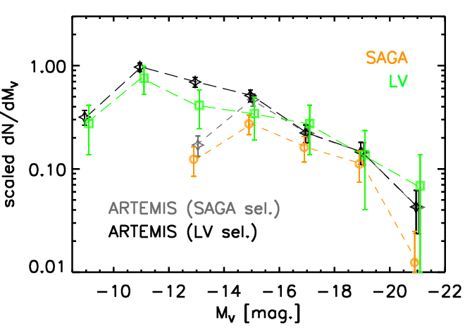
It is interesting to note that both Mao et al. 2021 and Carlsten et al. 2021 reported evidence for a slight excess of bright satellites ( mag.) with respect to the simulations they compared to, which were based on dark matter-only simulations populated using abundance matching techniques. We examine whether this is the case here by comparing the mean differential -band luminosity functions of ARTEMIS, SAGA, and the Local Volume in Fig. 5. We convert the -band luminosities of SAGA into the band using and we scale the luminosity functions in amplitude to account for the small differences in mean host -band magnitude. Two different luminosity functions are computed for ARTEMIS, corresponding to the different selection criteria for SAGA and LV. Note also that for this comparison we select only satellites within 150 kpc of the host, to ensure a fair comparison between the three data sets. We find generally good agreement (within the -sigma Poisson uncertainties) with both SAGA and LV. There is no obvious sign of an excess of bright satellites in the observational data sets with respect to ARTEMIS. Fig. 5 also nicely shows the impact of the different selection criteria for magnitudes fainter than . As noted by Carlsten et al. 2021, there is a difference between SAGA and the Local Volume at magnitudes fainter than this limit, which we attribute to a surface brightness limit in SAGA.
In terms of the bright-end of the luminosity function, it is presently unclear what the origin of the difference is between the predictions of ARTEMIS and that of abundance matching examined in Mao et al. 2021 and Carlsten et al. 2021. Carlsten et al. 2021 discuss two possible explanations for the difference between the abundance matching-based predictions and their observations, namely that: i) the intrinsic scatter in stellar mass at fixed halo mass could be larger than assumed in the fiducial abundance matching analyses; and/or ii) the local galaxy stellar mass function (from GAMA) used in the abundance matching analyses is slightly incomplete at stellar masses of M⊙ (e.g., Sedgwick et al. 2019). Either of these options could also explain the difference between the predictions of ARTEMIS and abundance matching. Clearly a more careful comparison between the predictions is required in order to ascertain the origin of the difference, which we leave for future work.
 |
 |
Moving on, the slopes of the luminosity functions, typically measured via the successive magnitude gaps, provide additional information about satellite populations. Prior measurements of the largest magnitude gaps in the luminosity functions have suggested another potential problem for the CDM model. Specifically, a few of the largest magnitude gaps measured in the SAGA ‘stage 1’ sample (Geha et al. 2017) appear to be larger than the scatter around the mean predicted by theoretical models. On the other hand, it has been argued that, statistically, such large magnitude gaps are expected in a CDM cosmology (Ostriker et al. 2019).
In Fig. 6 we investigate the largest magnitude gaps in the simulations and compare with the observations, namely the Local Volume, SAGA, and the Milky Way and M31. Here the largest magnitude gap is defined as the gap between adjacent (or ) values of dwarf galaxies (hence, excluding the host). The values for simulations are shown with star symbols and various values measured in observations are shown with coloured squares. Overall, the simulated values compare well with both sets of observations. The medians of the largest magnitude gaps in the simulations are for -band and for -band (note though that the two sets of observations have different magnitude limits and spatial coverage of dwarf galaxies). The median value of the largest gaps in our simulations is very good agreement with the median value of the models used by Geha et al. 2017, of mag. However, the scatter around the median largest gap in our simulations is larger than the scatter in the models used by Geha et al. 2017. While understanding the differences between the scatter in these models and in simulations is certainly useful, we note that the discrepancy between the former and the observations may be alleviated with the latest (SAGA) data. The larger SAGA sample (compared with the stage 1 SAGA sample presented in Geha et al. 2017) contains several systems with large magnitude gaps, including one with a gap mag, which was the upper limit in the models used in Geha et al. 2017.
As for the largest -band magnitude gaps, some of the values in the simulations can exceed mag, with no counterparts yet in the Local Volume sample with confirmed satellites only (coloured squares on the left panel of Fig. 6). However, by including other ‘possible’ satellites from Carlsten et al. 2021, it appears that M51 may possess such a large gap (green circle in the same panel).
Finally, we note that the comparisons in Fig. 6 applied the ‘LV selection’ and ‘SAGA selection’ criteria to the simulations. Virtually identical results are obtained if only a magnitude cut is applied (and no surface brightness cut), as the largest magnitude gaps are almost always determined at the bright end of the luminosity functions where the surface brightness limit is unimportant.

3.3 Abundance scaling relations
Having explored the luminosity functions of satellite around Milky Way-mass galaxies, we now examine how the abundance of satellites (i.e., their total number above some luminosity limit) correlates with the properties of the central host galaxy and with that of the overall host halo.
The top three panels of Fig. 7 show the relations between the abundance of satellites, defined here as , and the total stellar mass (computed within a fixed aperture of kpc), the -band magnitude, which is expected to correlate well with the stellar mass, and the virial mass of the host. Only subhaloes within of the center of the host are included in the top row. As expected, we find a strong correlation with the host . The computed Spearman rank correlation coefficient is . (A similar factor is found if we include dwarf galaxies within kpc of their host.) The correlation with host stellar mass () is also significant, with a Spearman coefficient of . Physically, we expect the abundance of haloes to be more strongly tied to the overall halo rather than with the central galaxy and the scatter in the stellar mass – halo mass relation is responsible for the somewhat weaker correlation between the satellite abundance and the host stellar mass. The correlation is similar in strength with that of (its Spearman coefficient is ), reflecting the known sensitivity of this magnitude band to the total stellar mass.
The dashed black lines in top row of Fig. 7 represent the best-fit power law distributions to the abundance scaling relatons for satellites within and with . Specifically, we find:
| (1) |
| (2) |
| (3) |
for the three scaling relations, where the best-fit parameters were determined using a simple minimisation scheme and incorporating Poisson errors on the simulation abundances.
In the bottom three panels of Fig. 7 we apply various observationally-motivated choices and limitations. In the left panel we plot again , but now counting all dwarf galaxies out to kpc and brighter than . The correlation does not change significantly compared with the case above, when only systems within were considered (the Spearman coefficient is now , compared with previously). The best-fit power law to this relation is:
| (4) |
In the middle and right panels we apply the LV and SAGA selection criteria described in Section 2.2. With these constraints, the simulated and observed relations agree with each other, but the correlations are considerably weaker. The Spearman coefficients in the simulations are , in approximate agreement with the Spearman coefficient of obtained for the SAGA sample (see also Geha et al. 2017).
 |
 |
The best-fit power law to the simulations when applying the LV selection criteria is:
| (5) |
whereas the best-fit power law when applying the SAGA selection criteria to ARTEMIS is:
| (6) |
We also derive the best-fit power law from the SAGA data itself, finding:
| (7) |
where when fitting the SAGA data or the simulations with SAGA selection criteria applied we exclude the small number of hosts with no satellites. The ARTEMIS simulations reproduce the observed SAGA relation both in slope and amplitude (to within -sigma).
We highlight that the implementation of a surface brightness cut for the ARTEMIS satellites is important for the comparison to SAGA. Without a surface brightness cut, the best-fit power law becomes:
| (8) |
which is an increase of 30% in abundance at the relative to the case without a surface brightness cut, and larger than this for brighter systems (note the steeper trend when the surface brightness cut is neglected).
These results demonstrate that, by limiting the observations to the brightest of dwarf galaxies, the correlations between the number of satellites and host galaxy properties are much less evident. It also suggests that observations with significant limitations (either in magnitude or in physical extent) typically have a higher scatter in the abundance of satellites at fixed host properties than the intrinsic scatter predicted by cosmological models that do not impose such restrictions.
In the left panel of Fig. 8 we investigate the relation between the number of satellites and the bulge-to-total ratios of the host galaxies. Such a relation was suggested by Javanmardi & Kroupa 2020, who found a very strong correlation between these two parameters (with a Spearman coefficient of ), although on a very small sample of galaxies. For our comparison, we include four Milky Way-mass analogues from the Local Volume sample of Carlsten et al. 2021 with complete samples of bright () satellites within kpc of their hosts, and with measured values (Kormendy et al. 2010; Fisher & Drory 2011), to which we add similar data for the Milky Way and M31. For the simulations, we compute ratios using a kinematical decomposition of the bulge/halo and the disc. Specifically, we assign to the bulge only the star particles within the inner kpc and with no significant rotation, i.e. with a fraction of energy in rotation of less than of the total energy, i.e. . We note however that the ratios computed by kinematic decomposition may differ from the values determined in observations, typically using decomposition of light profiles.
We do not find any significant correlation between and , either in the simulations or the observations (the Spearman coefficients are essentially ). We checked that this result is not sensitive to the exact luminosity or spatial cuts; for example, if we select simulated satellites with and within a distance of their hosts, we still find a low Spearman coefficient (of ). We note that Javanmardi et al. 2019 also investigated such correlations using the Illustris simulations and have not found a correlation between the abundance of satellites and the host galaxy’s . Rather than this being a problem with the CDM model, as suggested by Javanmardi & Kroupa 2020, our results suggest that the observed relation can be easily skewed by including a few systems with extreme values (e.g. systems like M33 with or Cen A with , neither of which are of Milky Way-mass).
The right panel of Fig. 8 shows the distribution for the simulated galaxies versus the distribution in the Local Volume. For the simulations, we show two cuts in the kinematic selection of bulge stars: one with for stars in the inner kpc (this is the same cut as used in the left panel of Fig. 8), the other with , respectively. Both choices are somewhat arbitrary and will not correspond exactly with the bulge/disc decomposition based on light profiles more commonly employed in observations. Including stars with energies dominated by rotation is likely to contaminate the bulge with disc stars (as shown in fig. B1 of Font et al. 2020, stars with are located in star-forming regions). For the observational sample, we include all galaxies in the Tully et al. 2009 catalogue66 6 See the ‘Local Universe’ catalogue at the Extragalactic Distance Database, http://edd.ifa.hawaii.edu. with measured values, plus the Milky Way and M31 ( galaxies in total). We use the values from Table 1 of Peebles 2020, which are measurements from Kormendy et al. 2010 and Fisher & Drory 2011. The simulated and observed distributions are in reasonably good agreement (note that the samples are also of similar size). All distributions have a narrow range in which suggests a correlation with - which it has been found to display a large scatter - to be unlikely.
Our simulations obtain a low median value, particularly when the bulge selection is limited to stars without significant rotation. This is encouraging, although we caution that the result needs to be confirmed with a bulge/disc decomposition based on light profiles, as in observations. Cosmological simulations have consistently encountered problems in producing disc galaxies with small bulges (see, e.g. Brooks & Christensen 2016 and references therein). Peebles 2020 has recently compared the values in the Local Volume galaxies (included by us above) with those in the Auriga (Gargiulo et al. 2019) or FIRE-2 (Garrison-Kimmel et al. 2018) simulations, and shown that the problem still exists in these simulations. The values in ARTEMIS are in the same range as in those simulations if we use the cut, but significantly lower if we use the selection. This suggests that the nature of the kinematic threshold is important in the bulge selection in simulations. We plan to investigate this issue in more detail in a future study.
3.4 Radial distribution of dwarf galaxies around Milky Way analogues
We now examine the radial distribution of dwarf galaxies around their hosts. As in previous sections, we begin by comparing the simulations to the Milky Way and M31 before moving on to the Milky Way analogues beyond the Local Group.
3.4.1 Comparison with the Milky Way and M31


With the ARTEMIS simulations, we can now revisit the claimed tension (discussed in the introduction) between the predictions of CDM models for radial distributions of satellites of Milky Way-mass galaxies and the measured radial distributions. As already mentioned, the Milky Way appears to be a rare system, with the majority () of its classical satellites (out to kpc) being clustered in the inner kpc or so (Yniguez et al. 2014). From a volume point of view, the majority of classical satellites apparently reside within central of the volume contained within .
The top panel of Fig. 9 shows the radial distributions of simulated satellites, i.e systems within with in ARTEMIS (grey lines) compared with those of Milky Way and M31 (blue and cyan lines, respectively). For observations we use the same dwarf galaxies mentioned in Section 3.2. Since we do not know the precise values for for the Milky Way and M31, we adopt a range of plausible values given the range of total mass estimates in the recent literature. Interestingly, we find that both the Milky Way and M31 (the former being significantly more concentrated than the latter) lie within the bounds of the simulated systems, even though they tend to exist on the extremities of the simulated distribution.
In the bottom panel of Fig. 9 we compare the radial distributions within a fixed distance of kpc. For both simulations and observations, we include only satellites with . Here both the Milky Way and M31 again fall within the scatter of the simulations. The inclusion of Crater 2 and Antlia 2 – which lie at distances of kpc (Torrealba et al. 2016) and kpc (Torrealba et al. 2019), respectively – alleviates some of the previously claimed tension between the Milky Way and previous simulations. With these additions, of Milky Way’s classical dwarfs (within kpc) are now within kpc.
It is also possible that a few classical dwarf galaxies could remain undetected observationally. For example, the observations do not include many systems like Crater 2 and Antlia 2, which have effective surface brightnesses mag arcsec-2 (Torrealba et al. 2016; Torrealba et al. 2019) and were discovered only recently.
Assuming that the number of undetected ultra-diffuse classical dwarfs is not large, how can we explain the difference between the radial distributions of Milky Way and M31 satellites? Moreover, our simulations indicate a large scatter in the radial distributions of dwarf galaxies, in a relatively narrow host mass range, even when we have normalised the radial coordinate by and have therefore removed the first order dependence of halo mass. Is this scatter purely stochastic, or does the scatter depend (at least in part) on other properties of the host? In Fig. 10 we examine how the concentration of the satellite system (defined below) depends on the concentration of host dark matter halo, . We have also examined the dependence of the satellite concentration on the halo formation age, (i.e., the lookback time to the formation redshift the halo, which is defined below). The halo concentration and halo formation time are known to be strongly correlated with each other and provide simple measures of the formation history of halo, with more highly-concentrated haloes tending to have assembled their mass earlier on (e.g., Navarro et al. 1996; Wechsler et al. 2002). For brevity, we do not show the trend with in Fig. 10, but we find it to be similar (in terms of the strength of the correlation) to the trend with the dark matter concentration.

The host dark matter concentrations are estimated by first producing spherically-averaged density profiles of the dark matter (excluding the contribution of satellites) and fitting an NFW form to the density profiles over the radial range . The inner boundary is imposed in order to avoid the region where baryons significantly affect the dark matter distribution, such that the NFW form generally does not provide a good fit. We fit for the scale radius, , and define the concentration in the usual way, as . In analogy to the dark matter concentration, we define the satellite concentration as , where is the satellite scale radius, which we derive by fitting an NFW form to the cumulative satellite radial distributions shown in the top panel of Fig. 9.
Specifically, we treat the cumulative satellite radial distribution in analogy to the enclosed mass of a NFW profile whose value is equal to the total mass (or here total number of satellites) at [i.e., ]:
| (9) |
where
| (10) |
and , such that .
Note that, since the profile is required to pass through at , which fixes the amplitude of the profile, the radial distribution depends only on the concentration parameter, . For each ARTEMIS halo and for the Milky Way and M31, we derive the best-fit concentration by simple chi-squared minimisation, adopting Poisson uncertainties on the cumulative radial profiles when fitting the model to the profiles.
The halo formation times are calculated as follows. We first construct a mass growth history for the most massive progenitor of the host halo. This is done by selecting all dark matter particles within at and, using their unique IDs, identifying the friends-of-friends group with the largest fraction of these particles in previous snapshots (earlier times). With the mass growth history, , we identify the redshift where half of the final mass is in place (Lacey & Cole 1993). We define the formation time, , as the lookback time to this redshift.
Our results suggest that the radial distribution of satellites does indeed ‘know about’ the concentration of the host dark halo (and its formation time) at fixed halo mass, although the correlation is not particularly strong, with a Spearman coefficient of . (We derive a similar correlation coefficient between the formation time of the halo and the satellite concentration.) Nevertheless, there is a tendency for haloes that are more concentrated and/or that have formed early on, to also have more radially-concentrated satellite populations at present time.
The filled, coloured points in Fig. 10 represented estimates of the concentrations for the Milky Way and M31. The dark matter halo concentrations, , for the Milky Way and M31 are from Cautun et al. 2020 and Tamm et al. 2012, respectively. Consistent with the findings from Fig. 9, the Milky Way and M31 lie within the scatter of the simulations but do tend to be on the extremities of the simulation distribution.

While the concentration of the satellite radial distribution appears to be partly set by that of the underlying dark matter, it is clear that this does not account for the bulk of the scatter in the satellite concentration at fixed halo mass (otherwise their would be a stronger correlation between the two concentration estimates). Another possibility is that the true underlying radial distribution is relatively poorly sampled by the finite number of measured satellites used to trace it. In other words, that the stochasticity in the positions of satellites along their orbits combined with the finite number of satellites used results in a noisy estimate of . We explore this possibility in Fig. 11, where we show the evolution of for individual haloes as a function of lookback time, . Here we employ a selection criteria of and that the satellites are within . It is clear to see that, with this satellite selection criteria, an individual halo can vary significantly in its estimated concentration even on timescales of Gyr, which is about the dynamical timescale. For a given halo, the mean RMS scatter about its mean concentration (averaged between and Gyr) is , such that a halo with can easily vary by and with no significant growth in halo mass or abundance of satellites over that period.
While the relatively weak correlation between and in Fig. 10 suggests that stochasticity plays a large factor in the satellite concentration, we note that the concentration of the host dark matter profile also evolves stochastically on relatively short timescales (see, e.g., Wang et al. 2020). In analogy to Fig. 11, we have therefore examined the variation in the host concentration with time. We find the mean RMS scatter about a given system’s mean concentration to be when the concentration is estimated from a profile including all dark matter particles, reducing to when the contribution of satellites is removed from the host dark matter profile. Thus, while the host concentration varies on relatively short timescales as well, these variations are not large enough to explain the bulk of the scatter in the satellite profile concentrations.
In summary, stochasticity is the most plausible explanation for the relatively large difference in the radial distributions of satellites of the Milky Way and M31 (i.e., the relatively small number of satellites used results in noisy estimates of the true radial profiles). This stochasticity can be overcome by either increasing the number of satellites used to characterise the radial distribution (i.e., by including fainter satellites) or by using additional information about the orbits of satellites to measure, for example, their time-averaged radius rather than the instantaneous one. By employing either (or both) of these measures, we might hope to better constrain the true underlying radial distribution and explore its link to the formation history of galaxies.
In Appendix B we explore an alternative definition for the concentration of the satellite radial distribution, which is based on the radius enclosing half of the satellites (as opposed to the NFW scale radius). While this quantity is more easily measured observationally, our conclusions above are unchanged with this alternative definition.
3.4.2 Comparisons withe the Milky Way analogues outside the Local Group

Here we extend our comparison of radial distribution of simulated dwarfs with measurements in Milky Way analogues beyond the Local Group. The larger number of such systems allow us to gauge the intrinsic scatter in the observed distributions and compare it with the scatter obtained in the simulations.
Fig. 12 shows the cumulative distributions of projected distances of satellites in ARTEMIS compared with those of satellites in the six Milky Way-analogues from the Local Volume from Carlsten et al. 2020b. For the latter, we include only satellites that are distance-confirmed. For the simulations, we compute projected distances from the 3D distances. We randomly rotate the viewing angle through each system, drawing 1000 distributions per ARTEMIS halo and sum these to produce a ‘heat map’ to show the resulting distribution. We ‘column-normalise’ the heat map (i.e., at a given project radius along the x axis we divide the pixels along the y axis by the sum of their values along that column) to better show the trend with projected distance. Overall, there is reasonable agreement between simulations and observations, in the sense that the observed distributions are bracketed by the simulations. Note that M51 exists on the very extremity of the simulated population, although it does have a few additional ‘possible satellites’ (i..e, without distance confirmation) which, if confirmed, would bring M51 more in line with the simulations.


Fig. 13 provides a more quantitative analysis of these radial distributions. Following Carlsten et al. 2020b, we plot the normalized differential distributions of satellites (number per host per kpc) in the six Local Volume galaxies (with green) and in ARTEMIS (with black lines), versus satellite projected distances. The top panel uses the default LV selection criteria for the simulations (i.e., , mags. arcsec-2 and kpc). The comparison is somewhat hindered by the sparsity of Local Volume data. Note that error bars on the Local Volume data correspond to Poisson errors. The simulations, on the other hand, include hosts where the satellites are viewed from a thousand random angles each. Nevertheless, this analysis shows that cosmological models are in reasonably good agreement with the observations in the top panel of Fig. 13. There is a tendency for the simulations to predict a somewhat higher abundance of satellites relative to the observations at larger radii ( kpc), but this is likely due to the Local Volume observations not fully extending to kpc for all hosts in that sample. In the legend in the top panel of Fig. 13 we provide the mean number of satellites contained within kpc and kpc (the latter in parenthesis) for the Local Volume and ARTEMIS samples. There is reasonably good agreement within 100 kpc. For reference, the dashed black histogram shows the impact of dropping the surface brightness limit when selecting satellites from the simulations. Overall the effect is fairly modest, typically increasing the satellite abundance by 10-15% with a mild dependence on projected distance.


, shown as a column-normalised heat map, in comparison with the observed distribution of projected distances of satellites of Milky Way analogues in SAGA, shown with orange lines. Middle: Normalized differential distribution functions of satellites per kpc per host in ARTEMIS compared with SAGA. The solid black histogram represents the simulations when the full SAGA selection criteria is applied, while the dashed black histogram shows the result when the surface brightness cut is removed. Bottom: Same as the middle panel except that the histograms have been scaled in amplitude according to eqn. 6 in order to account for the difference in the mean host K-band magnitude of ARTEMIS and SAGA (see text).
In the bottom panel of Fig. 13 we restrict the comparison to only the brightest satellites (). As discussed in Carlsten et al. 2020b, the Local Volume satellite populations appear to be more radially concentrated in the case of the brightest () dwarfs compared with those of the entire sample (). On the other hand, the simulations obtain similar distributions independent of the satellite magnitude cut. In terms of the difference with the Local Volume observations, we caution that there are very large Poisson uncertainties associated with the observed distribution, as there are typically only 2 to 3 satellites per halo meeting this selection criteria, derived from a sample of only 6 hosts. Furthermore, as already noted, the full area within 150 kpc was not surveyed for all 6 hosts.
In Fig. 14 we show the cumulative (top panel) and differential (middle panel) projected radial distributions of satellites in ARTEMIS with the SAGA selection criteria applied and make comparisons with the respective distributions from SAGA (orange curves). Overall the agreement with SAGA is reasonably good. There appears to be a slight difference in the radial dependence, with ARTEMIS having a stronger contribution from smaller projected radii (though perhaps not as strong as in the Local Volume results presented above).
The dashed-black histogram in the middle panel of Fig. 14 shows the impact of dropping the surface brightness cut on the predicted differential radial distribution from ARTEMIS. The effect is rather large, particularly at distances of kpc, where the abundance of satellites can increase by more than 50% as a result of dropping the surface brightness limit. The relatively strong radial dependence of this effect suggests that environmental processes (e.g., tidal heating) are driving it, but we leave a detailed analysis of the causes of this effect for future work.
Finally, in the bottom panel of Fig. 14 we show the impact of scaling the mean differential curves in the middle panel by a correction factor based on eqn. 6 that accounts for differences in the mean host K-band magnitudes of ARTEMIS and SAGA. As the mean host K-band magnitude of ARTEMIS is larger (brighter) than for SAGA (both of which are brighter than the adopted pivot point of ), the correction factor is larger for ARTEMIS than SAGA, resulting in a slightly improved agreement in the amplitude of the predicted and observed radial distributions.
4 Conclusions
The advent of deep observational surveys of local Milky Way ‘analogues’ and their satellite populations allows us to place the Milky Way in a broader cosmological context and to test the realism of cosmological simulations. In the present study, we have used the ARTEMIS suite of cosmological hydrodynamical simulations, introduced recently in Font et al. 2020, to make comparisons with the satellite luminosity functions, radial distribution functions, and abundance scaling relations of satellite galaxies in the Milky Way, M31, and Milky Way analogues sampled in the Local Volume (Carlsten et al. 2020a; Carlsten et al. 2020b; Carlsten et al. 2021) and SAGA (Geha et al. 2017; Mao et al. 2021) surveys. The main findings of these comparisons are as follows:
- •
An analysis of the magnitude–surface brightness relations of the SAGA and Local Volume surveys indicates that in order to enable a fair comparison with the simulations, both magnitude and surface brightness limits need to be factored in (Fig. 1).
- •
The distribution of host -band luminosities, a good proxy for stellar mass, of ARTEMIS galaxies is very similar to that of SAGA and Local Volume samples (Fig. 2), ensuring a fair comparison of their satellite populations. Nevertheless, we also explored the impact of differences in -band magnitudes throughout.
- •
The simulated satellite luminosity functions for the 45 ARTEMIS haloes are very similar to that observed for the Milky Way and M31 (Fig. 3) and for the Local Volume and SAGA surveys (Fig. 4) even though no aspect of the simulations was adjusted to obtain this. Furthermore, the simulations appear to naturally capture the large halo-to-halo diversity in the shape and amplitudes of the luminosity functions, having systems as abundant as M31 and as sparse as M94.
- •
Carlsten et al. 2021 and Mao et al. 2021 have reported evidence for a slight excess of bright () satellites with respect to previous simulations. In contrast, we find that ARTEMIS reproduces the abundance of bright satellites in the SAGA and Local Volume surveys to within Poisson uncertainties (Fig. 5).
- •
Contrary to previous claims, we find CDM-based simulations have no difficulties in reproducing the large magnitude gaps present in some observed satellite luminosity functions (Fig. 6).
- •
The abundance of satellites depends strongly on host properties, including stellar mass and (especially) total halo mass. However, applying practical observational selection criteria, such as fixed bright magnitude limits and fixed physical apertures, reduces the strength of these correlations (Fig. 7). We provide power law fits to the various scaling relations in eqns. 1–6. Contrary to some recent claims, we find no significant correlation between satellite abundance and host morphology (at fixed halo mass) in either the simulations or observations (Fig. 8).
- •
The radial distribution of satellites in the simulations is compatible with that observed for the Milky Way and M31 (Fig. 9). The Milky Way has a considerably more concentrated radial profile than M31. While this could potentially be explained if Milky Way’s underlying dark matter halo was significantly more concentrated than that of M31, recent measurements suggest that it is M31 that has the higher dark matter concentration (Fig. 10). It is more likely that stochasticity due to the use of a finite number of satellites is the main cause of the difference between M31 and the Milky Way. We have shown that the inferred radial concentration of the satellite population a given halo can vary significantly on a dynamical timescale when imposing observational selection criteria (Fig. 11).
- •
The present study has focused mainly on the luminosity functions and radial distribution functions of satellites around Milky Way-mass haloes. Broadly speaking, the simulations reproduce the observed distributions and with no fine tuning to do so. To yield sensible satellite populations in this regard requires not only having a realistic ‘backbone’ for structure formation (which CDM appears to provide) but also that processes such as star formation and stellar feedback are at least reasonable, otherwise the simulations would populate the dark matter haloes with galaxies of incorrect stellar mass/luminosity. However, a possibly much more challenging test for the simulations will be whether they can also reproduce the diversity of internal properties of satellites, including their star formation rates, colours, gas fractions, chemical abundances, and so on, and correctly describe how these quantities depend on host properties, e.g., halo mass, concentration, etc. We plan to examine these questions in future work.
Acknowledgments
The authors would like to thank the referee for constructive comments that substantially improved the paper. The authors would also like to thank the members of the EAGLE team for making their cosmological simulation code available for the ARTEMIS project. They also thank the Local Volume and SAGA survey teams for making their data sets publicly available. The authors would also like to thank Scott Carlsten for providing data and comments on the draft and Paul Bennet and Denija Crnojević for useful discussions. This project has received funding from the European Research Council (ERC) under the European Union’s Horizon 2020 research and innovation programme (grant agreement No 769130). This work used the DiRAC@Durham facility managed by the Institute for Computational Cosmology on behalf of the STFC DiRAC HPC Facility. The equipment was funded by BEIS capital funding via STFC capital grants ST/P002293/1, ST/R002371/1 and ST/S002502/1, Durham University and STFC operations grant ST/R000832/1. DiRAC is part of the National e-Infrastructure.
Data availability
The data underlying this article may be shared on reasonable request to the corresponding author.
References
- Behroozi et al. (2019) Behroozi P., Wechsler R. H., Hearin A. P., Conroy C., 2019, MNRAS, 488, 3143
- Bennet et al. (2019) Bennet P., Sand D. J., Crnojević D., Spekkens K., Karunakaran A., Zaritsky D., Mutlu-Pakdil B., 2019, ApJ, 885, 153
- Bennet et al. (2020) Bennet P., Sand D. J., Crnojević D., Spekkens K., Karunakaran A., Zaritsky D., Mutlu-Pakdil B., 2020, ApJ, 893, L9
- Bland-Hawthorn & Gerhard (2016) Bland-Hawthorn J., Gerhard O., 2016, ARA&A, 54, 529
- Boylan-Kolchin et al. (2011) Boylan-Kolchin M., Bullock J. S., Kaplinghat M., 2011, MNRAS, 415, L40
- Boylan-Kolchin et al. (2012) Boylan-Kolchin M., Bullock J. S., Kaplinghat M., 2012, MNRAS, 422, 1203
- Brada & Milgrom (2000) Brada R., Milgrom M., 2000, ApJ, 541, 556
- Bressan et al. (2012) Bressan A., Marigo P., Girardi L., Salasnich B., Dal Cero C., Rubele S., Nanni A., 2012, MNRAS, 427, 127
- Brooks & Christensen (2016) Brooks A., Christensen C., 2016, Bulge Formation via Mergers in Cosmological Simulations. p. 317, doi:10.1007/978-3-319-19378-6_12
- Brooks & Zolotov (2014) Brooks A. M., Zolotov A., 2014, ApJ, 786, 87
- Callingham et al. (2019) Callingham T. M., et al., 2019, MNRAS, 484, 5453
- Carlsten et al. (2020a) Carlsten S. G., Greco J. P., Beaton R. L., Greene J. E., 2020a, ApJ, 891, 144
- Carlsten et al. (2020b) Carlsten S. G., Greene J. E., Peter A. H. G., Greco J. P., Beaton R. L., 2020b, ApJ, 902, 124
- Carlsten et al. (2021) Carlsten S. G., Greene J. E., Peter A. H. G., Beaton R. L., Greco J. P., 2021, ApJ, 908, 109
- Cautun et al. (2020) Cautun M., et al., 2020, MNRAS, 494, 4291
- Chabrier (2003) Chabrier G., 2003, PASP, 115, 763
- Conn et al. (2012) Conn A. R., et al., 2012, ApJ, 758, 11
- Crnojević et al. (2019) Crnojević D., et al., 2019, ApJ, 872, 80
- D’Souza & Bell (2018) D’Souza R., Bell E. F., 2018, Nature Astronomy, 2, 737
- Danieli et al. (2017) Danieli S., van Dokkum P., Merritt A., Abraham R., Zhang J., Karachentsev I. D., Makarova L. N., 2017, ApJ, 837, 136
- Deason et al. (2013) Deason A. J., Belokurov V., Evans N. W., Johnston K. V., 2013, ApJ, 763, 113
- Deason et al. (2019) Deason A. J., Fattahi A., Belokurov V., Evans N. W., Grand R. J. J., Marinacci F., Pakmor R., 2019, MNRAS, 485, 3514
- Diaz et al. (2014) Diaz J. D., Koposov S. E., Irwin M., Belokurov V., Evans N. W., 2014, MNRAS, 443, 1688
- Dolag et al. (2009) Dolag K., Borgani S., Murante G., Springel V., 2009, MNRAS, 399, 497
- Drimmel & Spergel (2001) Drimmel R., Spergel D. N., 2001, ApJ, 556, 181
- Eadie & Jurić (2019) Eadie G., Jurić M., 2019, ApJ, 875, 159
- Erkal et al. (2019) Erkal D., et al., 2019, MNRAS, 487, 2685
- Fattahi et al. (2016) Fattahi A., et al., 2016, MNRAS, 457, 844
- Fisher & Drory (2011) Fisher D. B., Drory N., 2011, ApJ, 733, L47
- Flores & Primack (1994) Flores R. A., Primack J. R., 1994, ApJ, 427, L1
- Font et al. (2011) Font A. S., et al., 2011, MNRAS, 417, 1260
- Font et al. (2017) Font A. S., McCarthy I. G., Le Brun A. M. C., Crain R. A., Kelvin L. S., 2017, Publ. Astron. Soc. Australia, 34, e050
- Font et al. (2020) Font A. S., et al., 2020, MNRAS, 498, 1765
- Gargiulo et al. (2019) Gargiulo I. D., et al., 2019, MNRAS, 489, 5742
- Garrison-Kimmel et al. (2014) Garrison-Kimmel S., Horiuchi S., Abazajian K. N., Bullock J. S., Kaplinghat M., 2014, MNRAS, 444, 961
- Garrison-Kimmel et al. (2018) Garrison-Kimmel S., et al., 2018, MNRAS, 481, 4133
- Garrison-Kimmel et al. (2019) Garrison-Kimmel S., et al., 2019, MNRAS, 487, 1380
- Geha et al. (2017) Geha M., et al., 2017, ApJ, 847, 4
- Gibbons et al. (2014) Gibbons S. L. J., Belokurov V., Evans N. W., 2014, MNRAS, 445, 3788
- Gil de Paz et al. (2007) Gil de Paz A., et al., 2007, ApJS, 173, 185
- Governato et al. (2012) Governato F., et al., 2012, MNRAS, 422, 1231
- Graham & Colless (1997) Graham A., Colless M., 1997, MNRAS, 287, 221
- Heisler et al. (1985) Heisler J., Tremaine S., Bahcall J. N., 1985, ApJ, 298, 8
- Hinshaw et al. (2013) Hinshaw G., et al., 2013, ApJ Supplement Series, 208, 19
- Javanmardi & Kroupa (2020) Javanmardi B., Kroupa P., 2020, MNRAS, 493, L44
- Javanmardi et al. (2019) Javanmardi B., Raouf M., Khosroshahi H. G., Tavasoli S., Müller O., Molaeinezhad A., 2019, ApJ, 870, 50
- Jethwa et al. (2018) Jethwa P., Erkal D., Belokurov V., 2018, MNRAS, 473, 2060
- Kafle et al. (2018) Kafle P. R., Sharma S., Lewis G. F., Robotham A. S. G., Driver S. P., 2018, MNRAS, 475, 4043
- Karachentsev & Kudrya (2014) Karachentsev I. D., Kudrya Y. N., 2014, AJ, 148, 50
- Karachentsev et al. (2013) Karachentsev I. D., Makarov D. I., Kaisina E. I., 2013, AJ, 145, 101
- Kauffmann et al. (1993) Kauffmann G., White S. D. M., Guiderdoni B., 1993, MNRAS, 264, 201
- Kim et al. (2018) Kim S. Y., Peter A. H. G., Hargis J. R., 2018, Phys. Rev. Lett., 121, 211302
- Klypin et al. (1999) Klypin A., Kravtsov A. V., Valenzuela O., Prada F., 1999, ApJ, 522, 82
- Koposov et al. (2008) Koposov S., et al., 2008, ApJ, 686, 279
- Koposov et al. (2009) Koposov S. E., Yoo J., Rix H.-W., Weinberg D. H., Macciò A. V., Escudé J. M., 2009, ApJ, 696, 2179
- Kormendy et al. (2010) Kormendy J., Drory N., Bender R., Cornell M. E., 2010, ApJ, 723, 54
- Kravtsov et al. (2004) Kravtsov A. V., Gnedin O. Y., Klypin A. A., 2004, ApJ, 609, 482
- Lacey & Cole (1993) Lacey C., Cole S., 1993, MNRAS, 262, 627
- Lancaster et al. (2019) Lancaster L., Belokurov V., Evans N. W., 2019, MNRAS, 484, 2556
- Lovell et al. (2014) Lovell M. R., Frenk C. S., Eke V. R., Jenkins A., Gao L., Theuns T., 2014, MNRAS, 439, 300
- Macciò et al. (2010) Macciò A. V., Kang X., Fontanot F., Somerville R. S., Koposov S., Monaco P., 2010, MNRAS, 402, 1995
- Mao et al. (2021) Mao Y.-Y., Geha M., Wechsler R. H., Weiner B., Tollerud E. J., Nadler E. O., Kallivayalil N., 2021, ApJ, 907, 85
- Marigo et al. (2017) Marigo P., et al., 2017, ApJ, 835, 77
- Martin et al. (2013) Martin N. F., et al., 2013, ApJ, 772, 15
- McConnachie (2012) McConnachie A. W., 2012, AJ, 144, 4
- McConnachie et al. (2009) McConnachie A. W., et al., 2009, Nature, 461, 66
- McConnachie et al. (2018) McConnachie A. W., et al., 2018, ApJ, 868, 55
- Moore (1994) Moore B., 1994, Nature, 370, 629
- Moore et al. (1999) Moore B., Ghigna S., Governato F., Lake G., Quinn T., Stadel J., Tozzi P., 1999, ApJ, 524, L19
- Moster et al. (2018) Moster B. P., Naab T., White S. D. M., 2018, MNRAS, 477, 1822
- Navarro et al. (1996) Navarro J. F., Frenk C. S., White S. D. M., 1996, ApJ, 462, 563
- Ostriker et al. (2019) Ostriker J. P., Choi E., Chow A., Guha K., 2019, ApJ, 885, 97
- Peebles (2020) Peebles P. J. E., 2020, MNRAS, 498, 4386
- Pontzen & Governato (2012) Pontzen A., Governato F., 2012, MNRAS, 421, 3464
- Poole-McKenzie et al. (2020) Poole-McKenzie R., Font A. S., Boxer B., McCarthy I. G., Burdin S., Stafford S. G., Brown S. T., 2020, J. Cosmology Astropart. Phys., 2020, 016
- Posti & Helmi (2019) Posti L., Helmi A., 2019, A&A, 621, A56
- Read et al. (2006) Read J. I., Wilkinson M. I., Evans N. W., Gilmore G., Kleyna J. T., 2006, MNRAS, 367, 387
- Rocha et al. (2013) Rocha M., Peter A. H. G., Bullock J. S., Kaplinghat M., Garrison-Kimmel S., Oñorbe J., Moustakas L. A., 2013, MNRAS, 430, 81
- Ruchti et al. (2015) Ruchti G. R., et al., 2015, MNRAS, 450, 2874
- Samuel et al. (2020) Samuel J., et al., 2020, MNRAS, 491, 1471
- Sawala et al. (2016) Sawala T., et al., 2016, MNRAS, 457, 1931
- Schaye et al. (2015) Schaye J., et al., 2015, MNRAS, 446, 521
- Sedgwick et al. (2019) Sedgwick T. M., Baldry I. K., James P. A., Kelvin L. S., 2019, MNRAS, 484, 5278
- Smercina et al. (2018) Smercina A., Bell E. F., Price P. A., D’Souza R., Slater C. T., Bailin J., Monachesi A., Nidever D., 2018, ApJ, 863, 152
- Spergel & Steinhardt (2000) Spergel D. N., Steinhardt P. J., 2000, Phys. Rev. Lett., 84, 3760
- Stafford et al. (2020) Stafford S. G., Brown S. T., McCarthy I. G., Font A. S., Robertson A., Poole-McKenzie R., 2020, MNRAS,
- Starkenburg et al. (2013) Starkenburg E., et al., 2013, MNRAS, 429, 725
- Stewart et al. (2008) Stewart K. R., Bullock J. S., Wechsler R. H., Maller A. H., Zentner A. R., 2008, ApJ, 683, 597
- Tamm et al. (2012) Tamm A., Tempel E., Tenjes P., Tihhonova O., Tuvikene T., 2012, A&A, 546, A4
- Tollerud et al. (2008) Tollerud E. J., Bullock J. S., Strigari L. E., Willman B., 2008, ApJ, 688, 277
- Tollerud et al. (2014) Tollerud E. J., Boylan-Kolchin M., Bullock J. S., 2014, MNRAS, 440, 3511
- Torrealba et al. (2016) Torrealba G., Koposov S. E., Belokurov V., Irwin M., 2016, MNRAS, 459, 2370
- Torrealba et al. (2019) Torrealba G., et al., 2019, MNRAS, 488, 2743
- Trentham & Tully (2009) Trentham N., Tully R. B., 2009, MNRAS, 398, 722
- Tully et al. (2009) Tully R. B., Rizzi L., Shaya E. J., Courtois H. M., Makarov D. I., Jacobs B. A., 2009, AJ, 138, 323
- Vasiliev (2019) Vasiliev E., 2019, MNRAS, 484, 2832
- Walterbos & Kennicutt (1987) Walterbos R. A. M., Kennicutt R. C. J., 1987, A&AS, 69, 311
- Wang et al. (2020) Wang K., Mao Y.-Y., Zentner A. R., Lange J. U., van den Bosch F. C., Wechsler R. H., 2020, MNRAS, 498, 4450
- Watkins et al. (2010) Watkins L. L., Evans N. W., An J. H., 2010, MNRAS, 406, 264
- Watkins et al. (2019) Watkins L. L., van der Marel R. P., Sohn S. T., Evans N. W., 2019, ApJ, 873, 118
- Wechsler et al. (2002) Wechsler R. H., Bullock J. S., Primack J. R., Kravtsov A. V., Dekel A., 2002, ApJ, 568, 52
- Weisz et al. (2019) Weisz D. R., et al., 2019, MNRAS, 489, 763
- Wetzel et al. (2016) Wetzel A. R., Hopkins P. F., Kim J.-h., Faucher-Giguère C.-A., Kereš D., Quataert E., 2016, ApJ, 827, L23
- Wilkinson & Evans (1999) Wilkinson M. I., Evans N. W., 1999, MNRAS, 310, 645
- Wyse (2001) Wyse R. F. G., 2001, in Funes J. G., Corsini E. M., eds, Astronomical Society of the Pacific Conference Series Vol. 230, Galaxy Disks and Disk Galaxies. pp 71–80 (arXiv:astro-ph/0012270)
- Yniguez et al. (2014) Yniguez B., Garrison-Kimmel S., Boylan-Kolchin M., Bullock J. S., 2014, MNRAS, 439, 73
- van den Bosch & Ogiya (2018) van den Bosch F. C., Ogiya G., 2018, MNRAS, 475, 4066
Appendix A ARTEMIS host properties
In Table 1 we list various properties of the ARTEMIS host haloes and central galaxies.
| Galaxy | ||||||||
| [kpc] | [kpc] | [mag] | [mag] | [mag] | [mag] | |||
| G1 | 1.19 | 1.36 | 218.59 | 284.27 | -21.22 | -21.69 | -24.05 | -21.86 |
| G2 | 1.65 | 1.90 | 243.89 | 317.47 | -21.37 | -21.94 | -24.32 | -22.14 |
| G3 | 1.70 | 1.96 | 246.25 | 320.55 | -20.57 | -21.29 | -24.01 | -21.56 |
| G4 | 1.43 | 1.64 | 232.49 | 302.41 | -19.96 | -20.82 | -23.68 | -21.12 |
| G5 | 1.64 | 1.89 | 243.36 | 316.78 | -20.41 | -21.17 | -23.91 | -21.44 |
| G6 | 1.64 | 1.89 | 243.47 | 316.93 | -21.14 | -21.80 | -24.45 | -22.05 |
| G7 | 0.99 | 1.14 | 206.05 | 267.82 | -20.34 | -20.97 | -23.53 | -21.20 |
| G8 | 1.63 | 1.87 | 242.80 | 316.05 | -20.42 | -20.92 | -23.42 | -21.12 |
| G9 | 1.11 | 1.27 | 213.53 | 277.57 | -21.35 | -21.83 | -24.16 | -22.01 |
| G10 | 1.15 | 1.32 | 216.27 | 281.12 | -19.40 | -20.28 | -23.19 | -20.60 |
| G11 | 1.17 | 1.34 | 217.28 | 282.45 | -20.42 | -21.23 | -24.08 | -21.53 |
| G12 | 1.32 | 1.52 | 226.48 | 294.60 | -21.07 | -21.68 | -24.20 | -21.90 |
| G13 | 1.17 | 1.34 | 217.28 | 282.45 | -20.64 | -21.16 | -23.54 | -21.35 |
| G14 | 1.22 | 1.39 | 220.14 | 286.36 | -20.04 | -20.79 | -23.60 | -21.06 |
| G15 | 1.12 | 1.28 | 214.32 | 278.60 | -21.31 | -21.83 | -24.18 | -22.02 |
| G16 | 1.27 | 1.45 | 223.31 | 290.47 | -21.07 | -21.57 | -23.94 | -21.75 |
| G17 | 1.17 | 1.34 | 217.28 | 282.44 | -21.22 | -21.70 | -24.05 | -21.88 |
| G18 | 0.97 | 1.11 | 204.03 | 265.19 | -20.76 | -21.26 | -23.69 | -21.45 |
| G19 | 0.96 | 1.10 | 203.66 | 264.72 | -20.39 | -20.97 | -23.49 | -21.18 |
| G20 | 1.06 | 1.21 | 210.16 | 273.17 | -20.69 | -21.32 | -23.91 | -21.56 |
| G21 | 1.01 | 1.16 | 207.06 | 269.14 | -18.94 | -19.84 | -22.72 | -20.16 |
| G22 | 1.01 | 1.15 | 206.84 | 268.85 | -20.07 | -20.77 | -23.50 | -21.03 |
| G23 | 0.99 | 1.14 | 205.92 | 267.66 | -20.51 | -21.09 | -23.66 | -21.31 |
| G24 | 1.03 | 1.18 | 208.27 | 270.72 | -21.14 | -21.64 | -24.05 | -21.83 |
| G25 | 0.91 | 1.04 | 200.02 | 259.81 | -20.92 | -21.40 | -23.76 | -21.59 |
| G26 | 0.89 | 1.02 | 198.86 | 258.29 | -20.76 | -21.32 | -23.89 | -21.53 |
| G27 | 0.79 | 0.91 | 191.18 | 248.32 | -20.94 | -21.43 | -23.77 | -21.62 |
| G28 | 0.76 | 0.87 | 188.83 | 245.27 | -20.83 | -21.32 | -23.66 | -21.50 |
| G29 | 0.88 | 1.01 | 197.87 | 257.03 | -20.71 | -21.22 | -23.73 | -21.42 |
| G30 | 0.81 | 0.92 | 192.16 | 249.60 | -20.38 | -20.99 | -23.57 | -21.22 |
| G31 | 0.83 | 0.95 | 193.99 | 251.98 | -20.80 | -21.21 | -23.50 | -21.37 |
| G32 | 0.78 | 0.89 | 190.51 | 247.45 | -20.63 | -21.15 | -23.58 | -21.34 |
| G33 | 0.78 | 0.89 | 189.92 | 246.68 | -20.12 | -20.82 | -23.51 | -21.08 |
| G34 | 0.79 | 0.90 | 190.65 | 247.62 | -20.60 | -21.14 | -23.61 | -21.34 |
| G35 | 0.68 | 0.78 | 181.57 | 235.68 | -19.97 | -20.59 | -23.15 | -20.83 |
| G36 | 3.64 | 4.21 | 317.18 | 413.78 | -20.24 | -21.11 | -24.00 | -21.42 |
| G37 | 0.66 | 0.76 | 180.11 | 233.78 | -18.89 | -19.81 | -22.76 | -20.13 |
| G38 | 0.71 | 0.81 | 184.35 | 239.28 | -20.65 | -21.22 | -23.70 | -21.43 |
| G39 | 0.75 | 0.85 | 187.25 | 243.17 | -20.04 | -20.67 | -23.21 | -20.91 |
| G40 | 0.76 | 0.86 | 187.99 | 244.18 | -20.71 | -21.17 | -23.45 | -21.33 |
| G41 | 0.69 | 0.78 | 182.18 | 236.47 | -19.27 | -20.12 | -22.99 | -20.43 |
| G42 | 0.72 | 0.82 | 184.68 | 239.71 | -20.11 | -20.69 | -23.29 | -20.92 |
| G43 | 1.97 | 2.27 | 258.79 | 337.10 | -22.45 | -22.83 | -25.00 | -22.97 |
| G44 | 1.62 | 1.86 | 235.20 | 306.16 | -20.87 | -21.53 | -24.14 | -21.78 |
| G45 | 1.37 | 1.57 | 222.76 | 289.77 | -21.90 | -22.43 | -24.79 | -22.62 |
Appendix B Alternative concentration definition
In Section 3.4.1 we characterised the satellite radial distributions of the ARTEMIS haloes and the Milky Way and M31 via a concentration parameter derived by fitting an NFW profile to the radial distributions. Here we explore an alternative definition of concentration, which is potentially more easily measured for systems with few satellites. Specifically, here we define the satellite concentration as , where is the radius enclosing 50% of the satellites within .
Indeed, as shown in Fig. 15, we find that this definition of concentration has a reduced scatter compared to the NFW-based definition (20% here as opposed to 60% for the NFW concentration). Nevertheless, our conclusions remain the same: the correlation between this alternative concentration and the dark matter halo concentration is present but weak and stochasticity (see Fig. 16) is the main cause of scatter in this concentration at fixed halo mass. Also in agreement with the results presented in the main text, we find that the Milky Way and M31 have concentrations consistent with the simulated population.
Note that, although a concentration based on is perhaps easier to measure (less noisy) than the NFW-based concentration, it is also less likely to be correlated with the formation history of a halo, as it is less sensitive to the inner regions which collapsed earlier. In other words, it has a smaller ‘lever arm’ with respect to the formation history compared to the NFW-based concentration.

