No Subclass Left Behind: Fine-Grained Robustness in Coarse-Grained Classification Problems
Abstract
In real-world classification tasks, each class often comprises multiple finer-grained “subclasses.” As the subclass labels are frequently unavailable, models trained using only the coarser-grained class labels often exhibit highly variable performance across different subclasses. This phenomenon, known as hidden stratification, has important consequences for models deployed in safety-critical applications such as medicine. We propose George, a method to both measure and mitigate hidden stratification even when subclass labels are unknown. We first observe that unlabeled subclasses are often separable in the feature space of deep neural networks, and exploit this fact to estimate subclass labels for the training data via clustering techniques. We then use these approximate subclass labels as a form of noisy supervision in a distributionally robust optimization objective. We theoretically characterize the performance of George in terms of the worst-case generalization error across any subclass. We empirically validate George on a mix of real-world and benchmark image classification datasets, and show that our approach boosts worst-case subclass accuracy by up to 22 percentage points compared to standard training techniques, without requiring any prior information about the subclasses.
1 Introduction
In many real-world classification tasks, each labeled class consists of multiple semantically distinct subclasses that are unlabeled. Because models are typically trained to maximize global metrics such as average performance, they often underperform on important subclasses [58, 45]. This phenomenon—recently termed hidden stratification—can lead to skewed assessments of model quality and result in unexpectedly poor performance when models are deployed [41]. For instance, a medical imaging model trained to classify between benign and abnormal lesions may achieve high overall performance, yet consistently mislabel a rare but critical abnormal subclass as “benign” [18]. As another example, a well-known model for classifying chest radiographs was shown to perform substantially worse at recognizing pneumothorax (collapsed lung) on the subclass of pneumothorax images without a chest drain–which is worrisome since chest drains are the common form of treatment for the condition, so the drain-free subclass is in fact the clinically important one [41].
Modern robust optimization techniques can improve performance on poorly-performing groups when the group identities are known [48]. However, in practice, a key obstacle is that subclasses are often unlabeled, or even unidentified. This makes even detecting such performance gaps—let alone mitigating them—a challenging problem. Nevertheless, recent empirical evidence [41] encouragingly suggests that feature representations of deep neural networks often carry information about unlabeled subclasses (e.g., Figure 1). Motivated by this observation, we propose a method for addressing hidden stratification, by both measuring and improving worst-case subclass performance in the setting where subclass labels are unavailable. Our work towards this is organized into four main sections.

First, in Section 3 we propose a simple generative model of the data labeling process. Using this model, we show that when label annotations are insufficiently fine-grained—as is often the case in real-world datasets—hidden stratification can naturally arise. For instance, an image classification task might be to classify birds vs. frogs; if labels are only provided for these broad classes, they may fail to capture visually meaningful finer-grained, intra-class variation (e.g., “bird in flight” versus “bird in nest”). We show that in the setting of our generative model, standard training via empirical risk minimization (ERM) can result in arbitrarily poor performance on underrepresented subclasses.
Second, in Section 4 we use insights from this generative model to motivate George, a two-step procedure for alleviating hidden stratification by first estimating the subclass labels and then exploiting these estimates to train a robust classifier. To estimate subclass labels, we train a standard model on the task, and split each class (or “superclass,” for clarity) into estimated subclasses via unsupervised clustering in the model’s feature space. We then exploit these estimated subclasses by training a new model to optimize worst-case performance over all estimated subclasses using group distributionally robust optimization (GDRO) [48]. In this way, our framework allows ML practitioners to automatically detect poorly-performing subclasses and improve performance on them, without needing to resort to expensive manual relabeling of the data.
Third, in Section 5 we use our generative framework to prove that—under sufficiently strong conditions on the data distribution and the quality of the recovered clusters—George can reduce the subclass performance gap, attaining the same asymptotic sample complexity rates as if the true subclass labels were known.
Fourth, in Section 6 we empirically validate the ability of George to both measure and mitigate hidden stratification on four image classification tasks, comprising both robustness benchmarks and real-world datasets. We demonstrate that the first step of George—training an ERM model and clustering the superclass features—often recovers clusters that align closely with true subclasses. We evaluate the ability of these clusters to measure the worst-case subclass (i.e., “robust”) performance: on average, the gap between worst-case cluster performance and worst-case subclass performance is less than half the gap between overall and worst-case subclass performance, indicating that George enables more accurate measurement of robust performance. Next, we show that the second stage of George—retraining a robust model using cluster assignments as proxy subclass labels—reduces average worst-case subclass error rates by 22% on these datasets. For comparison, the state-of-the-art “oracle” GDRO method that does require subclass labels [48] reduces average worst-case subclass error rates by 51%. As an extension, we show that leveraging recent pretrained image embeddings [28] for clustering can substantially further improve the robust performance of George, in some cases to nearly match the performance of GDRO trained using the true subclass labels.11 1 Code for George can be found at https://github.com/HazyResearch/hidden-stratification.
2 Background
2.1 Related Work
Our work builds upon prior work from three main areas: robust optimization, representation learning, and unsupervised clustering. We provide a more extensive discussion of related work in Appendix A.
Distributionally Robust Optimization. Robustness and fairness is an active research area in machine learning [5, 22, 33, 27]. Distributionally robust optimization (DRO) attempts to guarantee good performance in the presence of distribution shift, e.g., from adversarial perturbations [54, 52] or evaluation on arbitrary subpopulations [17]. Because these notions of robustness can be pessimistic [24], others investigate group DRO (GDRO), which optimizes worst-case performance over a known set of groups (partitions) of the data [24, 48]. A major obstacle to applying GDRO methods in practice is that group labels are often unavailable; in our work, we aim to address this issue in the classification setting.
Representation Learning & Clustering. Our approach relies on estimating unknown subclass labels by clustering a feature representation of the data. Techniques for learning semantically useful image features include autoencoder-based methods [37, 51], the use of unsupervised auxiliary tasks [2, 10], and pretraining on massive datasets [28]. Such features may be used for unsupervised identification of classes, either using clustering techniques [7] or an end-to-end approach [26, 19]. It has also been observed that when a model is trained on coarse-grained class labels, the data within each class can often be separated into distinct clusters in model feature space (e.g., [41]). While we primarily focus on the latter approach, we also evaluate the utility of pretrained embeddings as a source of features for clustering.
2.2 Problem Setup
We are given datapoints and associated superclass labels .22 2 We assume since otherwise the “classification problem” is trivial. In addition, each datapoint is associated with a latent (unobserved) subclass label . We assume that is partitioned into disjoint nonempty sets such that if , then ; in other words, the subclass label determines the superclass label . Let denote the set of all subclasses comprising superclass , and denote the superclass corresponding to subclass .
Our goal is to classify examples from into their correct superclass. Given a function class , it is typical to seek a classifier that maximizes overall population accuracy:
| (1) |
By contrast, we seek to maximize the robust accuracy, defined as the worst-case expected accuracy over all subclasses:
| (2) |
Note that is fixed conditional on the value of . As we cannot directly optimize the population accuracy, we select a surrogate loss function and attempt to minimize this loss over the training data. For instance, the standard ERM approach to approximate (1) minimizes the empirical risk (i.e., training loss) :
| (3) |
To approximate (2), if we knew we could minimize the worst-case per-subclass training risk by solving:
| (4) |
where is the number of training examples from subclass . is the “robust loss” achieved by . Our goal is to learn a model such that is small with high probability. When the ’s are known, Eq. (4) can be tractably optimized using GDRO [24, 48]. However, we do not assume access to the ’s; we seek to approximately minimize without knowledge of the subclass labels.
3 Modeling Hidden Stratification
In Section 3.1, we introduce a generative model of the data labeling process. In Section 3.2, we use this model to explain how hidden stratification can occur, and show that in the setting of this model ERM can attain arbitrarily poor robust risk compared to GDRO.
3.1 A Model of the Data Generating and Labeling Process
In real datasets, individual datapoints are typically described by multiple different attributes, yet often only a subset of these are captured by the class labels. For example, a dataset might consist of images labeled “cat” or “dog.” These coarse class labels may not capture other salient attributes (color, size, breed, etc.); these attributes can be interpreted as latent variables representing different subclasses.
We model this phenomenon with a hierarchical data generation process. First, a binary vector is sampled from a distribution .33 3 In this paper, we use to denote a distribution and to denote its density. Each entry is an attribute, while each unique value of represents a different subclass. Then, a latent “feature vector” is sampled from a distribution conditioned on . Specifically, when conditioned on , each individual feature is Gaussian and independent of the ’s with . Finally, the datapoint is determined by the latent features via a fixed map . Meanwhile, the superclass label is equal to , where is a fixed discrete-valued function. In particular, may only depend on a subset of the attributes; the ’s which do not influence the label correspond to hidden subclasses. are observed, while are not. Figure 2a illustrates this generative process; Figure 2b presents an analogue on the Waterbirds dataset [48].
A key assumption is that the subclasses are “meaningful” in some sense, rather than just arbitrary groups of datapoints. Thus, rather than attempting to enforce good performance on all possible subsets of the data, we assume some meaningful structure on the subclass data distributions. We model this via the Gaussian assumption on , which is similar to that often made for the latent space of GANs [6]. Consequently, the data distribution is a mixture of Gaussians in the “canonical feature space” , which facilitates further theoretical analysis (Section 5). Our generative model also bears similarity to that of [24], who use a hierarchical data-generation model to analyze the behavior of DRO methods in the presence of distribution shift.


3.2 What Causes Hidden Stratification, and When Can It Be Fixed?
We now use our generative model to help understand why hidden stratification can occur, and present a simple example in which ERM is provably suboptimal in terms of the robust risk.
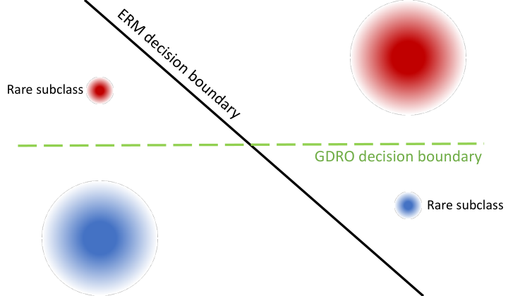
We distinguish between two main causes of hidden stratification: inherent hardness and dataset imbalance. First, certain subclasses are “inherently harder” to classify because they are more similar to other superclasses. We define the inherent hardness of a task as the minimum attainable robust error; inherent hardness thus lower bounds the worst-case subclass error of any model. See Appendix D for more discussion.
Second, imbalance in subclass sizes can cause ERM to underserve rare subclasses, since it optimizes for average-case performance. We provide a simple concrete example (3.1) below. Unlike inherent hardness, robust performance gaps arising from dataset imbalances can be resolved if subclass labels are known, by using these labels to minimize the objective in Equation (4) via GDRO.
Example 3.1.
Figure 3 depicts an example distribution generated by the model in Section 3.1. In this example, the binary attribute vector has dimension 2, i.e., , while only determines the superclass label , i.e., . The latent attribute induces two subclasses in each superclass, each distributed as a different Gaussian in feature space, with mixture proportions and respectively. For linear models with regularized logistic loss, there exists a family of distributions of this form such that as the proportion of the rare subclasses goes to , the worst-case subclass accuracy of ERM is only , while that of GDRO is . (See Appendix D.1 for the specific parameters of the per-subclass distributions in this example and a proof of the claim.)
Example 3.1 illustrates that when the dataset is imbalanced—i.e., the distribution of the underlying attributes is highly nonuniform—knowledge of subclass labels can improve robust performance. We thus ask: how well can we estimate subclass labels if they are not provided? In the extreme, if two subclasses of a superclass have the same distribution in feature space, we cannot distinguish them. However, the model must then perform the same on each subclass, since its prediction is a fixed function of the features! Conversely, if one subclass has higher average error, it must lie “further across” the decision boundary, meaning that the two subclasses must be separable to some degree; the larger the accuracy gap, the more separable the subclasses are. We formalize this in Appendix D.3.
4 George: A Framework for Mitigating Hidden Stratification
Inspired by the insights of Section 3, we propose George, an algorithm to mitigate hidden stratification. A schematic overview of George is provided in Figure 4.

Under the generative model of Section 3.1, each subclass is described by a different Gaussian in latent feature space. This suggests that a natural approach to identify the subclasses is to transform the data into feature space, and then cluster the data into estimated subclasses. However, this feature space is unknown. To obtain a surrogate for this feature space, we leverage the empirical observation that feature representations of deep neural networks trained on a superclass task can carry information about unlabeled subclasses [41]. Next, to improve performance on these estimated subclasses, we minimize the maximum per-cluster average loss, by using the clusters as groups in the GDRO objective [48]. We provide more details below, and pseudocode in Appendix B (Algorithm 1).
4.1 Step 1: Estimating Approximate Subclass Labels
In the first step of George, we train an ERM model on the superclass task and cluster the feature representations of each superclass to generate proxy subclass labels. Formally, we train a deep neural network to predict the superclass labels, where is a parametrized “featurizer” and outputs classification logits. We then cluster the features output by for the data of each superclass into clusters, where is chosen automatically. To each datapoint in the training and validation sets, we associate its cluster assignment . We use the ’s as surrogates for the true subclass labels .
4.1.1 Clustering Details
In practice, we apply UMAP dimensionality reduction [38] before clustering, as we find it improves results (Appendix B). Additionally, based on the insight of Section 3.2 that subclasses with high loss differences are more separable, we also use the loss component (i.e., the component of the activation vector orthogonal to the decision boundary) as an alternative representation.
We first tried using standard clustering methods (such as -means and Gaussian mixture model clustering) in our work. By visual inspection, we found that these methods often failed to capture smaller clusters, even if they were well-separated. However, missing small clusters like this is problematic for George, since these small clusters frequently correspond to rare, low-performing subclasses. Additionally, these methods require specification of . We apply over-clustering (clustering using a larger ) to remedy this problem in an efficient manner. Naive overclustering also has drawbacks as it still requires manual specification of , and if is set too large, several clusters can be spurious and result in overly pessimistic and unstable measurements of robust performance (as we explore in Appendix C.5). Thus, we develop a fully automated criterion based on the commonly used Silhouette (SIL) criterion [47] to search for the number of clusters , over-cluster to find smaller clusters that were missed, and filter out the spurious overclusters. Empirically, our clustering approach significantly improves performance over “vanilla” clustering; we hope that it may be of independent interest as well. We describe our procedures in more detail in Appendix B.
4.2 Step 2: Exploiting Approximate Subclass Labels
In the second step of George, we use the GDRO algorithm from [48] and our estimated subclass labels to train a new classifier with better worst-case performance on the estimated subclasses. Given data and loss function , GDRO minimizes with respect to parameters , where is the discrete set of groups and is the empirical distribution of examples from group . This coincides with the true objective (4) when the true subclass labels are used as the group labels . In our case, we use the cluster assignments as the group labels instead, i.e., minimize .44 4 In Appendix D, we present an extension to the GDRO algorithm of [48] to handle the case where the group assignments can be probabilistic labels in , instead of hard labels in . Similarly, using the clusters fit on the training set, we generate cluster assignments for the validation set points and use these to compute the validation worst-case per-cluster performance. George uses this metric, rather than overall validation performance, to select the best model checkpoint over the training trajectory.
5 Analysis of George
We now analyze a simple mixture model data distribution, based on the generative model presented in Section 3.1. We show that in this setting, unlike ERM, George converges to the optimal robust risk at the same sample complexity rate as GDRO when it is able to recover the true latent features (and when “soft” group predictions are used). Specifically, Example 3.1 shows that the robust risk of ERM can be arbitrarily worse than that of GDRO, for data generated according to the generative model in Section 3.1. By contrast, if the subclass labels estimated by George are sufficiently accurate, then the objective minimized in Step 2 of George well approximates the true GDRO objective (4). In Theorem 1, we use this to show that, when each subclass is described by a different Gaussian in feature space, George (with soft group predictions) achieves the same optimal asymptotic sample complexity rates as GDRO trained with true subclass labels. We sketch the argument below; full proofs are deferred to Appendix D.
First, suppose we could compute the true data distribution . Our goal is to minimize the maximum per-subclass training loss by solving Eq. (4). Even with infinite data, we cannot estimate the individual ’s to arbitrary accuracy, so we cannot directly compute the objective in (4). However, we can estimate the per-subclass losses as follows: for each training example , we use to compute the probability that it comes from subclass , and use that to weight the loss corresponding to that example. In Lemma 1, we show that when the training data is randomly sampled from , this yields an unbiased estimate of the average per-subclass empirical risk.
Lemma 1.
Let be the sample average loss of examples in subclass . Let . Let be the sample average of over all examples with superclass label . Then is an unbiased estimate of , and their difference converges to at the rate .
In practice, we do not have access to the true distribution , so we estimate it with , computed from data. Thus, the weights are replaced by weights estimated from , leading to an estimate of the quantity defined in Lemma 1. Nevertheless, if we can bound the total variation estimation error of , we can use this to bound the error in this loss estimate, as shown in Lemma 2 (Appendix D).55 5 In general, estimation of the data distribution to within small total variation error is a strong requirement, and is difficult to ensure in practice. However, it can be achieved in certain special cases, such as the mixture-of-Gaussian setting in Theorem 1. In Theorem 1, we leverage Lemma 2 and recent results on learning Gaussian mixtures [3] to show that, when each subclass is described by a different Gaussian, can be estimated well enough so that the minimizer of the perturbed robust loss converges to the minimizer of the true robust loss at the optimal sample complexity rate.
Theorem 1.
Let . Suppose and are Lipschitz, has bounded parameters, and is Gaussian and unique for each subclass . Then, if we estimate using the algorithm from [3], satisfies w.h.p.
Theorem 1 implies that if each subclass is Gaussian in feature space, and we have access to this feature space (i.e., we can invert the mapping from features to data ), then we can cluster the features to estimate , and the robust generalization performance of the model that minimizes the resulting perturbed training loss scales the same as does that of the minimizer of the true robust training loss , in terms of the amount of data required. This underscores the importance of recovering a “good” feature space; empirically, we show in Appendix C that the choice of model architecture can indeed dramatically impact the model feature space and thus the ability to recover subclasses.
6 Experiments
We empirically validate that George can mitigate hidden stratification across four datasets. In Section 6.2, we show that when subclass labels are unavailable, George improves robust performance over standard training methods. In Section 6.3, we analyze the clusters returned by George to understand the reasons for this improvement; we confirm that George identifies clusters that correspond to poorly-performing subclasses, which enables accurate measurement of robust performance. In Section 6.4, we ablate the contributions that George’s robust training objective and George’s improved measurement of validation robust performance each make to the performance gains of George. Finally, in Section 6.5, we evaluate the use of recent pretrained image embeddings [28] as a source of features for George, and find that this further improves performance of George on some applications. Additional details on datasets, model architectures, and experimental procedures are provided in Appendix B.
6.1 Datasets
Waterbirds. Waterbirds, a robustness benchmark introduced to evaluate GDRO in [48], contains images of land-bird and water-bird species on either land or water backgrounds. The task is to classify images as “land-bird” or “water-bird”; however, 95% of land (water)-birds are on land (water) backgrounds, causing ERM to frequently misclassify both land-birds on water and water-birds on land.
Undersampled MNIST (U-MNIST). We design U-MNIST as a modified version of MNIST [30], where the task is to classify digits as ‘5’ and ‘5’ (digits 0-9 are the subclasses). In addition, we remove 95% of ‘8’s; due to its rarity, it is challenging for ERM to perform well on the ‘8’ subclass.
CelebA. CelebA is a common face classification dataset also used as a robustness benchmark in [48]. The task is to classify faces as “blond” or “not blond.” Because only 6% of blond faces are male, ERM performs poorly on this rare subclass.
6.2 End-to-End Results
| Method | Requires | Metric | Waterbirds | U-MNIST | ISIC | CelebA | ||
| Subclass Labels? | Type | Non-patch | Histopath. | |||||
| ERM | ✗ | Robust | 63.3(1.6) | 93.9(0.6) | .922(.003) | .875(.005) | 40.3(2.3) | |
| Overall | 97.3(0.1) | 98.7(0.1) | .957(.002) | 95.7(0.0) | ||||
| George (ours) | ✗ | Robust | 76.2(2.0) | 95.7(0.6) | .912(.005) | .876(.006) | 53.7(1.3) | |
| Overall | 95.7(0.5) | 98.1(0.3) | .927(.008) | 94.6(0.2) | ||||
| Subclass-GDRO | ✓ | Robust | 90.7(0.4) | 96.8(0.4) | .923(.003) | .875(.004) | 89.3(0.9) | |
| Overall | 92.7(0.4) | 98.0(0.3) | .933(.005) | 92.8(0.1) | ||||
We first show that George substantially improves the worst-case subclass accuracy, while modestly affecting overall accuracy. (Recall that we refer to worst-case subclass accuracy as “robust accuracy” [Eq. (2)].) We train models on each dataset in Section 6.1 using (a) ERM, (b) George, and (c) GDRO with true subclass labels (“Subclass-GDRO”), and report both robust and overall performance metrics in Table 1. Compared to ERM, training with George improves robust accuracy by up to 22 points, and substantially reduces the gap between the robust error of the ERM model and that of the subclass-GDRO model—despite the fact that George does not require subclass labels. In Appendix C, we show that George also outperforms other subclass-agnostic baselines, such as GDRO trained using the superclasses as groups.
On Waterbirds, U-MNIST, and CelebA, George significantly improves worst-case subclass accuracy over ERM. On ISIC, all methods perform similarly in terms of both AUROC on the non-patch subclass and AUROC on the clinically meaningful histopathology subclass. On CelebA, although George improves upon ERM, it substantially underperforms subclass-GDRO. However, this gap can be closed when improved features are used: if we cluster pretrained BiT embeddings [28] rather than ERM features and use the resulting cluster assignments for the second stage of George, the robust accuracy improves to nearly match that of subclass-GDRO. We describe this experiment in Section 6.5.
In terms of overall performance, ERM generally performs best (as it is designed to optimize for average-case performance), followed by George and then subclass-GDRO. However, this difference is generally much smaller in magnitude than the increase in robust performance.
6.3 Clustering Results
Step 1 of George is to train an ERM model and cluster the data of each superclass in its feature space. We analyze these clusters to better understand George’s behavior. First, in Section 6.3.1 we show that George finds clusters that align well with poorly-performing human-labeled subclasses. This helps explain why the second step of George, running GDRO using the cluster assignments as groups, improves performance on these subclasses (as demonstrated in Section 6.2). Next, in Section 6.3.2 we show that George can discover meaningful subclasses that were not labeled by human annotators. Finally, in Section 6.3.3 we show that the worst-case performance measured on the clusters returned by George is a good approximation of the true robust performance.
6.3.1 Subclass Recovery
We evaluate the ability of George to identify clusters that correspond to the true subclasses. We focus on identification of poorly-performing subclasses, as these determine robust performance. In Table 2, we compute the precision and recall of the cluster returned by George that most closely aligns with each given subclass. Precision is the fraction of cluster examples with that subclass label; recall is the fraction of subclass examples assigned to the cluster. For each poorly-performing subclass, George identifies a cluster with high recall and better-than-random precision. (Interestingly, while the precision and recall are substantially better than random in all cases, they are often still quite far from the optimal value of 1.0, but Step 2 of George nevertheless achieves substantial worst-group performance gains.)
We note that the lower recall on ISIC is because the no-patch subclass is often split into multiple clusters; in fact, this subclass is actually composed of two semantically distinct groups as discussed below. If these sub-clusters are combined into one, the precision and recall of the resulting cluster at identifying no-patch examples are and respectively.
6.3.2 Unlabeled Subclass Discovery
In addition to yielding clusters aligned with human-annotated subclasses, our procedure can identify semantically meaningful subclasses that were not specified in the human-provided schema. On U-MNIST, 60% of trials of George partition the “7” subclass into two subclusters, each containing stylistically different images (Figure 6c, Appendix C). On ISIC, 70% of George trials reveal distinct benign clusters within the no-patch subclass (see Figure 6g-i). In these trials, at least 77% of images in one of these no-patch clusters required histopathology (biopsy & pathologist referral), while such images made up 7% of each other cluster. In other words, the no-patch subclass split into “histopathology” and “non-histopathology” clusters, where the former datapoints were harder for clinicians to classify. We comment on the real-world importance of the ISIC result in particular. Naively, the overall AUROC on ISIC obtained using the ERM model is 0.957, which suggests a high-performing model; however, our clustering reveals that a large fraction of the benign images contain a “spurious” brightly colored patch, which makes them very easy to classify. The model performs substantially worse on examples without such a patch, and worse still on “more difficult” examples for which a clinician also utilized a histopathology examination to make a diagnosis. Thus, if deployed in practice with a target sensitivity value in mind, the appropriate way to set an operating point for this model is in fact cluster-dependent; if a single operating point were set using the aggregate ROC curve, the true sensitivity on the histopathology subclass would be substantially lower than intended. This means that even simply measuring hidden stratification via Step 1 of George can provide crucial information that would help avoid spurious false negatives at test time—the worst type of error a medical screening application can make.
| Task | Subclass | Subclass Prevalence | % of trials | Precision | Recall |
| U-MNIST | “8” digit | 0.012 | 80 | 0.54 | 0.74 |
| Waterbirds | Water-birds on land | 0.05 | 100 | 0.19 | 0.91 |
| Waterbirds | Land-birds on water | 0.05 | 100 | 0.33 | 0.93 |
| ISIC | No-patch | 0.48 | 100 | 0.99 | 0.59 |
| ISIC | Histopathology | 0.23 | 70 | 0.77 | 0.92 |
| CelebA | blond males | 0.06 | 100 | 0.14 | 0.88 |
| CelebA (w/BiT) | blond males | 0.06 | 100 | 0.93 | 0.68 |
6.3.3 Estimating Robust Accuracy
We show that the clusters returned by George enable improved measurement of worst-case subclass performance. Specifically, we measure the worst-case performance across any cluster returned by George (which we call the “cluster-robust” performance) and compare this to the true robust performance and the overall performance. We present results for both ERM and George in Table 3. In most cases, the cluster-robust performance is much closer to the true robust performance than the overall performance is. On ISIC, cluster-robust performance even yields a better estimate of robust performance on the histopathology subclass than does performance on the patch/no-patch subclass. By comparing cluster-robust performance to overall performance, we can detect hidden stratification (and estimate its magnitude) without requiring subclass labels.
| Method | Metric | Waterbirds | U-MNIST | ISIC | CelebA | ||
| Type | Non-patch | Histopath. | |||||
| ERM | Robust | 63.3(1.6) | 93.9(0.6) | .922(.003) | .875(.005) | 40.3(2.3) | |
| Cluster-Robust | 76.8(1.4) | 92.3(2.5) | .893(.013) | 56.7(2.5) | |||
| Overall | 97.3(0.1) | 98.2(0.1) | .957(.002) | 95.7(0.1) | |||
| George | Robust | 76.2(2.0) | 95.7(0.6) | .912(.005) | .876(.006) | 53.7(1.3) | |
| Cluster-Robust | 78.3(1.1) | 93.5(1.9) | .897(.011) | 70.8(1.1) | |||
| Overall | 95.7(0.5) | 97.9(0.2) | .927(.008) | 94.6(0.2) | |||
In addition, improvements in robust performance from George compared to ERM are accompanied by increases in cluster-robust performance; by comparing the cluster-robust performance of ERM and George, we can estimate how much George improves hidden stratification.
6.4 Effects of Validation Metric
George’s improvement of robust performance has two potential explanations: (1) minimizing the cluster-robust training loss is a better surrogate objective for the true robust performance than minimizing the overall training loss, and (2) selecting the best model checkpoint based on validation cluster-robust performance is better than selecting based on overall validation performance. To decouple these two effects, in Table 8 we display the test robust performance for ERM and George when using the true robust validation performance as a checkpointing metric. This change generally improves performance for both methods, but George still significantly outperforms ERM on all datasets except ISIC. This shows that, for the goal of maximizing robust performance, the GDRO objective with cluster labels indeed performs better than the ERM objective.
In Table 8, we also display the effects of changing the frequencies of subclasses in the validation set. As described in Appendix B.2, by default we re-weight the validation and test sets of U-MNIST and Waterbirds so that the effective frequencies of each subclass are the same as they are in the training set. If we turn off this reweighting, the cluster-robust validation performance is a more accurate measure of the true robust performance, since the frequency of the underperforming subclass increases in the validation set. Using this unreweighted metric to select the best model checkpoint increases the true robust performance of George to 83.3%—an improvement of over 22 points compared to ERM checkpointed against average accuracy on the same unreweighted validation set. We stress that the true validation subclass labels are still assumed to be unknown in this experiment. Having training and validation sets with different distributions is realistic in many situations.
We remark that in typical supervised learning settings, model selection—encompassing both hyperparameter tuning and selection of a checkpoint from the training trajectory—is done with the help of a validation set on which the desired metric of interest can be computed. By contrast, the setting we study in George is more challenging not only due to the absence of training group labels, but also because the absence of validation group labels means that this selection metric (worst-group accuracy / AUROC) cannot even be computed exactly on the validation set. The results of this section are encouraging in that they suggest that George’s cluster-robust performance is an acceptable proxy metric for model selection.66 6 Our hyperparameter tuning procedure is described in Section B.3; we also do not use validation set group labels to tune any of George’s hyperparameters.
| Training | Validation | Waterbirds | U-MNIST | ISIC | CelebA | ||
| Method | Checkpoint Metric | Non-patch | Histopath. | ||||
| ERM | Acc. | 63.3(1.6) | 93.9(0.6) | .922(.003) | .875(.005) | 40.3(2.3) | |
| Unw. Acc. | 60.7(0.7) | 94.2(0.8) | - | - | |||
| Robust Acc. | 68.8(0.9) | 94.5(0.9) | .924(.003) | .880(.004) | 46.3(2.1) | ||
| George | Cluster-Robust Acc. | 76.2(2.0) | 95.7(0.6) | .912(.005) | .876(.006) | 53.7(1.3) | |
| Unw. Cluster-Robust Acc. | 83.3(1.3) | 95.7(0.6) | - | - | |||
| Robust Acc. | 83.8(1.0) | 96.3(0.5) | .915(.004) | .877(.006) | 54.9(1.9) | ||
6.5 Extension: Leveraging Pretrained Embeddings
As an alternative to training an ERM model, we assess whether recent pretrained image embeddings (BiT [28]) can provide better features for Step 1 of George. Specifically, we modify Step 1 of George to compute BiT embeddings for the datapoints, cluster the embeddings, and use these cluster assignments as estimated subclass labels in Step 2 of George. This modification (George-BiT) dramatically improves robust accuracy on CelebA to 87.3% (), nearly matching subclass-GDRO.99 9 Overall accuracy drops somewhat to 91.5%.
The CelebA BiT clusters align much better with the true subclasses (cf. Table 2), which helps explain this improvement. Similarly, cluster-robust accuracy measured using the BiT clusters is much closer to the true robust accuracy: for the George-BiT model, average cluster-robust performance on the BiT clusters is , and for ERM it is [compared to the true robust accuracy of 40.3%].
Despite its excellent performance on CelebA, the default George implementation outperforms George-BiT on the other datasets, suggesting that BiT is not a panacea: on these datasets, the task-specific information contained in the representation of the trained ERM model seems to be important for identifying meaningful clusters. See Appendix B.3.6 for additional evaluations and discussion. Extending Step 1 of George to enable automatically selecting between different representations (e.g., BiT vs. ERM) is a compelling future topic.
7 Conclusion
We propose George, a two-step approach for measuring and mitigating hidden stratification without requiring access to subclass labels. George’s first step, clustering the features of an ERM model, identifies clusters that provide useful approximations of worst-case subclass performance. George’s second step, using these cluster assignments as groups in GDRO, yields significant improvements in worst-case subclass performance. We analyze George in the context of a simple generative model, and show that under suitable assumptions George achieves the same asymptotic sample complexity rates as if we had access to true subclass labels. We empirically validate George on four datasets, and find evidence that it can reduce hidden stratification on real-world machine learning tasks. Interesting directions for future work include further exploring different ways to learn representations for the first stage of George, developing better unsupervised metrics to choose between representations and clustering methods, and characterizing when ERM learns representations that enable separation of subclasses.
Acknowledgments
We thank Arjun Desai, Pang Wei Koh, Shiori Sagawa, Zhaobin Kuang, Karan Goel, Avner May, Esther Rolf, and Yixuan Li for helpful discussions and feedback.
We gratefully acknowledge the support of DARPA under Nos. FA86501827865 (SDH) and FA86501827882 (ASED); NIH under No. U54EB020405 (Mobilize), NSF under Nos. CCF1763315 (Beyond Sparsity), CCF1563078 (Volume to Velocity), and 1937301 (RTML); ONR under No. N000141712266 (Unifying Weak Supervision); the Moore Foundation, NXP, Xilinx, LETI-CEA, Intel, IBM, Microsoft, NEC, Toshiba, TSMC, ARM, Hitachi, BASF, Accenture, Ericsson, Qualcomm, Analog Devices, the Okawa Foundation, American Family Insurance, Google Cloud, Swiss Re, Total, the HAI-AWS Cloud Credits for Research program, the Schlumberger Innovation Fellowship program, and members of the Stanford DAWN project: Facebook, Google, VMWare, and Ant Financial. The U.S. Government is authorized to reproduce and distribute reprints for Governmental purposes notwithstanding any copyright notation thereon. Any opinions, findings, and conclusions or recommendations expressed in this material are those of the authors and do not necessarily reflect the views, policies, or endorsements, either expressed or implied, of DARPA, NIH, ONR, or the U.S. Government.
References
- Arjovsky et al. [2019] Martin Arjovsky, Léon Bottou, Ishaan Gulrajani, and David Lopez-Paz. Invariant risk minimization. arXiv preprint arXiv:1907.02893, 2019.
- Asano et al. [2020] Yuki Asano, Christian Rupprecht, and Andrea Vedaldi. A critical analysis of self-supervision, or what we can learn from a single image. In International Conference on Learning Representations (ICLR), 2020.
- Ashtiani et al. [2018] Hassan Ashtiani, Shai Ben-David, Nick Harvey, Christopher Liaw, Abbas Mehrabian, and Yaniv Plan. Near-optimal sample complexity bounds for robust learning of Gaussian mixtures via compression schemes. In Advances in Neural Information Processing Systems (NeurIPS), 2018.
- Balashankar et al. [2019] Ananth Balashankar, Alyssa Lees, Chris Welty, and Lakshminarayanan Subramanian. What is fair? Exploring Pareto-efficiency for fairness constrained classifiers. arXiv preprint arXiv:1910.14120, 2019.
- Barocas et al. [2019] Solon Barocas, Moritz Hardt, and Arvind Narayanan. Fairness and Machine Learning. fairmlbook.org, 2019. http://www.fairmlbook.org.
- Bojanowski et al. [2018] Piotr Bojanowski, Armand Joulin, David Lopez-Paz, and Arthur Szlam. Optimizing the latent space of generative networks. In International Conference on Machine Learning (ICML), 2018.
- Caron et al. [2018] Mathilde Caron, Piotr Bojanowski, Armand Joulin, and Matthijs Douze. Deep clustering for unsupervised learning of visual features. In European Conference on Computer Vision (ECCV), pages 132–149, 2018.
- Chalupka et al. [2015] Krzysztof Chalupka, Pietro Perona, and Frederick Eberhardt. Visual causal feature learning. In Uncertainty in Artificial Intelligence (UAI), 2015.
- Chen et al. [2020a] Beidi Chen, Weiyang Liu, Zhiding Yu, Jan Kautz, Anshumali Shrivastava, Animesh Garg, and Anima Anandkumar. Angular visual hardness. In International Conference on Machine Learning (ICML), 2020a.
- Chen et al. [2020b] Ting Chen, Simon Kornblith, Mohammad Norouzi, and Geoffrey Hinton. A simple framework for contrastive learning of visual representations. In International Conference on Machine Learning (ICML), 2020b.
- Chen et al. [2019] Vincent Chen, Sen Wu, Alexander Ratner, Jen Weng, and Christopher Ré. Slice-based learning: A programming model for residual learning in critical data slices. In Advances in Neural Information Processing Systems (NeurIPS), pages 9392–9402, 2019.
- Chilamkurthy et al. [2018] Sasank Chilamkurthy, Rohit Ghosh, Swetha Tanamala, Mustafa Biviji, Norbert Campeau, Vasantha Kumar Venugopal, Vidur Mahajan, Pooja Rao, and Prashant Warier. Deep learning algorithms for detection of critical findings in head CT scans: a retrospective study. Lancet, 392(10162):2388–2396, December 2018.
- Codella et al. [2019] Noel Codella, Veronica Rotemberg, Philipp Tschandl, M. Emre Celebi, Stephen Dusza, David Gutman, Brian Helba, Aadi Kalloo, Konstantinos Liopyris, Michael Marchetti, et al. Skin lesion analysis toward melanoma detection 2018: A challenge hosted by the international skin imaging collaboration (ISIC). arXiv preprint arXiv:1902.03368, 2019.
- Devroye et al. [2018] Luc Devroye, Abbas Mehrabian, and Tommy Reddad. The total variation distance between high-dimensional Gaussians. arXiv preprint arXiv:1810.08693, 2018.
- Dong et al. [2014] Jian Dong, Qiang Chen, Jiashi Feng, Kui Jia, Zhongyang Huang, and Shuicheng Yan. Looking inside category: subcategory-aware object recognition. IEEE Transactions on Circuits and Systems for Video Technology, 25(8):1322–1334, 2014.
- Dong et al. [2015] Jian Dong, Qiang Chen, Jiashi Feng, Kui Jia, Zhongyang Huang, and Shuicheng Yan. Looking inside category: Subcategory-aware object recognition. Circuits and Systems for Video Technology, IEEE Transactions on, 25:1322–1334, 08 2015. doi: 10.1109/TCSVT.2014.2355697.
- Duchi et al. [2020] John Duchi, Tatsunori Hashimoto, and Hongseok Namkoong. Distributionally robust losses for latent covariate mixtures. arXiv preprint arXiv:2007.13982, 2020.
- Dunnmon et al. [2019] Jared Dunnmon, Darvin Yi, Curtis Langlotz, Christopher Ré, Daniel Rubin, and Matthew Lungren. Assessment of convolutional neural networks for automated classification of chest radiographs. Radiology, 290(2):537–544, February 2019.
- Gansbeke et al. [2020] Wouter Van Gansbeke, Simon Vandenhende, Stamatios Georgoulis, Marc Proesmans, and Luc Van Gool. Learning to classify images without labels. arXiv preprint arXiv:2005.12320, 2020.
- Gulshan et al. [2016] Varun Gulshan, Lily Peng, Marc Coram, Martin Stumpe, Derek Wu, Arunachalam Narayanaswamy, Subhashini Venugopalan, Kasumi Widner, Tom Madams, Jorge Cuadros, Ramasamy Kim, Rajiv Raman, Philip Nelson, Jessica Mega, and Dale Webster. Development and validation of a deep learning algorithm for detection of diabetic retinopathy in retinal fundus photographs. Journal of the American Medical Association, 316(22):2402–2410, December 2016.
- Han et al. [2019] Kai Han, Andrea Vedaldi, and Andrew Zisserman. Learning to discover novel visual categories via deep transfer clustering. In IEEE International Conference on Computer Vision (ICCV), pages 8401–8409, 2019.
- Hardt et al. [2016] Moritz Hardt, Eric Price, and Nati Srebro. Equality of opportunity in supervised learning. In Advances in Neural Information Processing Systems (NeurIPS), pages 3315–3323, 2016.
- Hoai and Zisserman [2013] Minh Hoai and Andrew Zisserman. Discriminative sub-categorization. In IEEE Conference on Computer Vision and Pattern Recognition (CVPR), pages 1666–1673, 2013.
- Hu et al. [2018] Weihua Hu, Gang Niu, Issei Sato, and Masashi Sugiyama. Does distributionally robust supervised learning give robust classifiers? In International Conference on Machine Learning (ICML), 2018.
- Jacobs et al. [1991] Robert Jacobs, Michael I. Jordan, Steven Nowlan, and Geoffrey Hinton. Adaptive mixtures of local experts. Neural Computation, 3(1):79–87, 1991.
- Ji et al. [2019] Xu Ji, João Henriques, and Andrea Vedaldi. Invariant information clustering for unsupervised image classification and segmentation. In IEEE International Conference on Computer Vision (ICCV), pages 9865–9874, 2019.
- Kearns et al. [2019] Michael Kearns, Aaron Roth, and Saeed Sharifi-Malvajerdi. Average individual fairness: Algorithms, generalization and experiments. In Advances in Neural Information Processing Systems (NeurIPS), 2019.
- Kolesnikov et al. [2020] Alexander Kolesnikov, Lucas Beyer, Xiaohua Zhai, Joan Puigcerver, Jessica Yung, Sylvain Gelly, and Neil Houlsby. Big transfer (BiT): General visual representation learning. In European Conference on Computer Vision (ECCV, 2020.
- Lahoti et al. [2020] Preeti Lahoti, Alex Beutel, Jilin Chen, Kang Lee, Flavien Prost, Nithum Thain, Xuezhi Wang, and Ed Chi. Fairness without demographics through adversarially reweighted learning. In Advances in Neural Information Processing Systems (NeurIPS), 2020.
- LeCun et al. [2010] Yann LeCun, Corinna Cortes, and C.J. Burges. MNIST handwritten digit database, 2010. URL http://yann.lecun.com/exdb/mnist.
- Levy et al. [2020] Daniel Levy, Yair Carmon, John Duchi, and Aaron Sidford. Large-scale methods for distributionally robust optimization. In Advances in Neural Information Processing Systems (NeurIPS), volume 33, pages 8847–8860, 2020.
- Liang and Ma [2019] Percy Liang and Tengyu Ma. Stanford CS 229T course notes, 2019. URL http://web.stanford.edu/class/cs229t/.
- Lipton et al. [2018] Zachary Lipton, Julian McAuley, and Alexandra Chouldechova. Does mitigating ML’s impact disparity require treatment disparity? In Advances in Neural Information Processing Systems (NeurIPS), pages 8125–8135, 2018.
- Liu et al. [2015] Ziwei Liu, Ping Luo, Xiaogang Wang, and Xiaoou Tang. Deep learning face attributes in the wild. In IEEE International Conference on Computer Vision (ICCV), 2015.
- Martinez et al. [2020] Natalia Martinez, Martin Bertran, and Guillermo Sapiro. Minimax pareto fairness: A multi objective perspective. In International Conference on Machine Learning (ICML), 2020.
- Martinez et al. [2021] Natalia Martinez, Martin Bertran, Afroditi Papadaki, Miguel Rodrigues, and Guillermo Sapiro. Blind Pareto fairness and subgroup robustness. In International Conference on Machine Learning (ICML), 2021.
- McConville et al. [2020] Ryan McConville, Raúl Santos-Rodríguez, Robert J Piechocki, and Ian Craddock. N2D: (not too) deep clustering via clustering the local manifold of an autoencoded embedding. In International Conference on Pattern Recognition (ICPR), 2020.
- McInnes et al. [2018] Leland McInnes, John Healy, and James Melville. UMAP: Uniform manifold approximation and projection for dimension reduction. arXiv preprint arXiv:1802.03426, 2018.
- Mintz et al. [2009] Mike Mintz, Steven Bills, Rion Snow, and Dan Jurafsky. Distant supervision for relation extraction without labeled data. In Joint Conference of the Annual Meeting of the Association for Computational Linguistics (ACL) and the International Joint Conference on Natural Language Processing (IJCNLP), volume 2, pages 1003–1011, 2009.
- Muller et al. [2020] Rafael Muller, Simon Kornblith, and Geoffrey Hinton. Subclass distillation. arXiv preprint arXiv:2002.03936, 2020.
- Oakden-Rayner et al. [2020] Luke Oakden-Rayner, Jared Dunnmon, Gustavo Carneiro, and Christopher Ré. Hidden stratification causes clinically meaningful failures in machine learning for medical imaging. In ACM Conference on Health, Inference, and Learning (CHIL), 2020.
- Polyzotis et al. [2019] Neoklis Polyzotis, Steven Whang, Tim Kraska, and Yeounoh Chung. Slice finder: Automated data slicing for model validation. In IEEE International Conference on Data Engineering (ICDE), 2019.
- Ratner et al. [2019] Alexander Ratner, Stephen Bach, Henry Ehrenberg, Jason Fries, Sen Wu, and Christopher Ré. Snorkel: Rapid training data creation with weak supervision. The VLDB Journal, 29:709–730, 2019.
- Recht et al. [2018] Benjamin Recht, Rebecca Roelofs, Ludwig Schmidt, and Vaishaal Shankar. Do CIFAR-10 classifiers generalize to CIFAR-10? arXiv preprint arXiv:1806.00451, 2018.
- Recht et al. [2019] Benjamin Recht, Rebecca Roelofs, Ludwig Schmidt, and Vaishaal Shankar. Do ImageNet classifiers generalize to ImageNet? In International Conference on Machine Learning (ICML), 2019.
- Rieger et al. [2020] Laura Rieger, Chandan Singh, William Murdoch, and Bin Yu. Interpretations are useful: penalizing explanations to align neural networks with prior knowledge. In International Conference on Machine Learning (ICML), 2020.
- Rousseeuw [1987] Peter Rousseeuw. Silhouettes: a graphical aid to the interpretation and validation of cluster analysis. Journal of Computational and Applied Mathematics, 20:53–65, 1987.
- Sagawa et al. [2020] Shiori Sagawa, Pang Wei Koh, Tatsunori Hashimoto, and Percy Liang. Distributionally robust neural networks for group shifts: On the importance of regularization for worst-case generalization. In International Conference on Learning Representations (ICLR), 2020.
- Schölkopf [2019] Bernhard Schölkopf. Causality for machine learning. arXiv preprint arXiv:1911.10500, 2019.
- Scope et al. [2016] Alon Scope, Michael Marchetti, Ashfaq Marghoob, Stephen Dusza, Alan Geller, Jaya Satagopan, Martin Weinstock, Marianne Berwick, and Allan Halpern. The study of nevi in children: Principles learned and implications for melanoma diagnosis. Journal of the American Academy of Dermatology, 75(4):813 – 823, 2016. ISSN 0190-9622. doi: https://doi.org/10.1016/j.jaad.2016.03.027. URL http://www.sciencedirect.com/science/article/pii/S019096221630010X.
- Shukla et al. [2018] Ankita Shukla, Gullal Singh Cheema, and Saket Anand. Semi-supervised clustering with neural networks. arXiv preprint arXiv:1806.01547, 2018.
- Sinha et al. [2018] Aman Sinha, Hongseok Namkoong, Riccardo Volpi, and John Duchi. Certifying some distributional robustness with principled adversarial training. In International Conference on Learning Representations (ICLR), 2018.
- Snell et al. [2017] Jake Snell, Kevin Swersky, and Richard Zemel. Prototypical networks for few-shot learning. In Advances in Neural Information Processing Systems (NeurIPS), pages 4077–4087, 2017.
- Staib and Jegelka [2017] Matthew Staib and Stefanie Jegelka. Distributionally robust deep learning as a generalization of adversarial training. In NeurIPS Workshop on Machine Learning and Computer Security, 2017.
- Wang et al. [2019] Haohan Wang, Songwei Ge, Zachary Lipton, and Eric Xing. Learning robust global representations by penalizing local predictive power. In Advances in Neural Information Processing Systems (NeurIPS), pages 10506–10518, 2019.
- Wang et al. [2020] Serena Wang, Wenshuo Guo, Harikrishna Narasimhan, Andrew Cotter, Maya Gupta, and Michael Jordan. Robust optimization for fairness with noisy protected groups. In Advances in Neural Information Processing Systems (NeurIPS), volume 33, pages 5190–5203. Curran Associates, Inc., 2020.
- Xie et al. [2017] Pengtao Xie, Aarti Singh, and Eric Xing. Uncorrelation and evenness: a new diversity-promoting regularizer. In International Conference on Machine Learning (ICML), 2017.
- Yao et al. [2011] Bangpeng Yao, Aditya Khosla, and Li Fei-Fei. Combining randomization and discrimination for fine-grained image categorization. In IEEE Conference on Computer Vision and Pattern Recognition (CVPR), pages 1577–1584. IEEE, 2011.
Appendix
Appendix A Extended Related Work
Our work builds on several active threads in the machine learning literature.
Hidden Stratification.
Our motivating problem is that of hidden stratification, wherein models trained on superclass labels exhibit highly variable performance on unlabeled subclasses [41]. This behavior has been observed in a variety of studies spanning both traditional computer vision [58, 44, 15, 23] and medical machine learning [41, 18, 20, 12]. Of note is the work of [44], who propose that the existence of “distribution shift” at the subclass level may substantially affect measures of test set performance for image classification models on CIFAR-10. They use a simple mixture model between an “easy” and a “hard” subclass to demonstrate how changes that would not be detectable at the superclass level could affect aggregate performance metrics. [9] extend these ideas by developing notions of visual hardness, and suggest that better loss function design would be useful for improving the performance of machine learning models on harder examples. [42] studies how to automatically find large, interpretable underperforming data slices in structured datasets.
Our approach is also inspired by the literature on causality and machine learning, and in particular by the common assumption that the data provided for both training and evaluation are independent and identically distributed (IID) [49]. This is often untrue in real-world settings; in particular, classes in real-world datasets are often composed of multiple subclasses, and the proportions of these subclasses may change between training and evaluation settings—even if the overall class compositions are the same. Many of the guarantees from statistical learning theory break down in the presence of such non-IID data [8], suggesting that models trained using traditional Empirical Risk Minimization (ERM) are likely to be vulnerable to hidden stratification. This motivates the use of the maximum (worst-case) per-subclass risk, rather than the overall average risk, as the objective to be optimized.
Neural Representation Clustering.
The first stage of the technique we propose for addressing hidden stratification (George) relies heavily on our ability to identify latent subclasses via unsupervised clustering of neural representations learned via ERM. This has been an area of substantial recent activity in machine learning, and has provided several important conclusions upon which we build in our work. The work of [37] and [51], for instance, demonstrate the utility of a simple autoencoded representation for performing unsupervised clustering in the feature space of a trained model. While the purpose of these works is often to show that deep clustering can be competitive with semi-supervised learning techniques, the mechanics of clustering in model feature space explored by these works are important for our present study. Indeed, we directly leverage the conclusion of [37] that Uniform Manifold Approximation and Projection (UMAP) [38] works well as a dimensionality reduction technique for deep clustering in the current study.
Further, the fact that work such as [21] directly uses neural representation clustering to estimate the presence of novel classes in a given dataset provides an empirical basis for our approach, which uses a model trained with ERM to approximately identify unlabeled subclasses within each superclass. Similarly, [26] demonstrate excellent semi-supervised image classification performance by maximizing mutual information between the class assignments of each pair of images. Their work demonstrates not only the utility of a clustering-style objective in image classification, but also suggests that overclustering – using more clusters than naturally exist in the data – can be beneficial for clustering deep feature representations in a manner that is helpful for semi-supervised classification.
A related, but different, approach is that of [15], who explicitly attempt to identify subcategories of classes via a graph and SVM-based “subcategory mining” framework in order to improve overall task performance. The subcategory mining algorithm is quite complicated and uses manually extracted features (rather than automatically learned features, e.g., from CNNs); in addition, this work is geared towards improving overall performance, rather than ensuring good performance on all subcategories. Nevertheless, it is an important piece of prior literature.
Distributionally Robust Optimization.
The second stage of Georgedepends on our ability to optimize the worst-case classification loss over existing subgroups. This formulation draws a clear connection between our work and the literature on fairness in machine learning [5], which is at least partially concerned with ensuring that trained models do not disadvantage a particular group in practice. While there exist a wide variety of definitions for algorithmic fairness [22, 33, 27], the common idea that models should be optimized such that they respect various notions of fairness is similar to the motivation behind our work.
Distributionally robust optimization studies the problem of optimizing for worst-case performance with respect to some “uncertainty set” of distributions. A multitude of recent papers have explored optimizing distributionally robust objectives in slightly different contexts. Most relevant to our work is the study of [48], who propose the group DRO algorithm for training classifiers with best worst-case subgroup performance (in other words, the “uncertainty sets” in this case are the per-group distributions). Crucially, this algorithm demonstrates improved worst-case subclass performance in cases where triplets () are known for every data point, with is the input data, is the true label, and is a true subgroup label. While [48] present preliminary evidence that group DRO can work well in the presence of noisy , the efficacy of the algorithm in this setting remains functionally unexplored. We leverage the group DRO algorithm as an optimizer for minimizing the worst-case loss with respect to our approximately identified subclasses.
We also discuss other works on DRO. [17], for instance, considers the general problem of optimizing the worst-case loss over any possible subdistribution of the data above a specified size; while conceptually important, the goal of optimizing over arbitrary subdistributions of a minimum size is rather pessimistic compared to assuming more structure on these subdistributions (such as in GDRO). [31] built upon these ideas to design efficient methods for large-scale DRO, but the uncertainty sets considered are also less structured compared to group DRO and therefore generally give poorer results when the goal is in fact to optimize worst-group performance on a specific set of groups. Concurrently with our work, [56] studies how to train models with respect to group-level fairness constraints, given only noisy versions of the groups; they show how to solve this problem efficiently via a DRO formulation and a reweighting approach based on soft group assignments. While their formulation encompasses several fairness objectives, such as “equal opportunity” (equal true positive rates across groups) and “equal outcome” (equal positive prediction rates across groups), it does not directly optimize for worst-group performance. Additionally, they assume that the noisy group labels are provided and their marginal distribution is the same as that of the true groups, whereas we do not assume any foreknowledge of the (noisy or true) groups.
Similar to the goal of optimizing worst-group performance is optimizing for group Pareto fairness, i.e., seeking solutions that are Pareto-efficient in terms of the performances on each group. [4] and [35] both study this (more general) problem in the case where the group labels are known. In addition, follow-ups to these papers that were concurrent to our work explored this problem in the setting where the group labels are unknown [29, 36]; however, both of these works focus on simpler structured datasets rather than more challenging settings such as image classification.
Other relevant techniques include invariant risk minimization, which attempts to train classifiers that are optimal across data drawn from a mixture of distributions (i.e., a non-IID setting) [1]; methods from slice-based learning that learn feature representations optimized for ensuring high performance on specific subsets, or “slices” of the data [11]; mixture-of-experts models, which explicitly handle learning models for multiple different subsets of data [25]; and techniques for building robust classifiers via domain adaptation [55]. While our work is closely related to these directions, a major difference is that we handle the setting where the different subclasses (i.e., groups, environments, slices, etc.) are unidentified.
Representation Learning with Limited or Noisy Labels.
A final research thread that is closely related to the work presented here focuses on deep representation learning in the absence of ground truth labels. Our methods are similar in spirit to those from weak supervision [39, 43], which focuses on training models using noisy labels that are often provided programmatically. Our work can be seen as analyzing a new form of fine-grained weak supervision for DRO-style objectives, which is drawn from unsupervised clustering of an ERM representation. Another related line of work is representation learning for few-shot learning [53]; however, our work fundamentally differs in the sense that we assume no access to ground truth subclass labels.
Other methods aim to automatically learn classes via an iterative approach. An early work of this type is [7], which uses iterative clustering and ERM training to learn highly effective feature representations for image classification. More recently, [19] used a self-supervised task to learn semantically meaningful features, and then generate labels using an iteratively refining approach. Our work differs from these in that we do assume access to ground truth superclass labels—which provide much more information than in the fully-unlabeled setting—and use clustering within each superclass to generate approximate labels. In addition, our primary end goal is not accurate identification of the subclasses, but ensuring good worst-case performance among all subclasses.
Finally, other works aim to promote a notion of “diversity” among feature representations by adding different regularizers. In [57], such a regularizer was introduced in the context of latent space models, to better capture infrequently observed patterns and improve model expressiveness for a given size. More recently, [40] introduced a regularizer that aims to promote diversity of the predicted logits. They showed that this method could also lead to estimation of subclasses within a superclass, without requiring subclass labels. However, this work focused on improving overall performance, and specifically improvement of knowledge distillation; by contrast, our goal is to improve robust performance. Nevertheless, integrating these recent ideas into our work is an interesting avenue for future work, to potentially further improve the feature learning stage.
Appendix B Experimental Details
B.1 George Pseudocode
We provide pseudocode for George in Algorithm 1, to complement the detailed description of our methodology in Section 4.1010 10 We note that the final step of George—training a model to minimize the maximum per-cluster risk—can also be done when “soft” (probabilistic) cluster labels are given instead of hard assignments; see Appendix D.5. Note that our model class (as per the notation in Section 2.2) is a class of neural networks, composed of a “featurizer” module and a “linear classification head” that takes the feature representation to a prediction.
Optional input: Pretrained featurizer
if featurizer provided then
2 end if
3
for to do
4 Get_Cluster_Labels() end for
5
6 return ()
Note that our framework is not constrained by the specific choice of clustering algorithm, dimensionality reduction algorithm, or robust optimization algorithm. While we use GDRO throughout this work, other training techniques that encourage good robust performance could be swapped in for GDRO during “Step 2” of George.
B.2 Dataset Details
Below, we describe the datasets used for evaluation in more detail. [We provide PyTorch dataloaders to support each one in our code.]
Each dataset contains labeled subclasses; although the George procedure does not use the subclass labels at any point, we use them to assess how well George (a) can estimate the subclass labels and (b) can estimate and improve worst-case subclass performance.
We remark that while we evaluate on binary classification tasks in this work, George can readily be applied in principle to tasks with any amount of superclasses and subclasses.
B.2.1 U-MNIST
Undersampled MNIST (U-MNIST) is a binary dataset that divides data from the standard MNIST dataset (which has 60,000 training points) into two superclasses: numbers less than five, and numbers greater than or equal to five. Crucially, the “8” subclass is subsampled at 5% of its usual frequency in MNIST. The rarity of the “8” subclass makes this task much more challenging than the default MNIST task, in terms of robust performance. We use data drawn from the original MNIST validation set as our test set; we create a separate validation set of 12,000 points by sampling from the MNIST training set, and use the remainder for training.
On the validation (and test) sets, we do not actually undersample the 8’s, as this would leave only 50-60 “8” examples; instead, we downweight these examples when computing validation/test accuracies and losses, to mimic the rarity that would be induced by actually undersampling but still allow for more stable accuracy measurements.
B.2.2 Waterbirds
The Waterbirds dataset (4,795 training points) used in this work was introduced in [48]. Similar to our approach for U-MNIST, Sagawa et al. [48] create more balanced validation and test sets to allow for stable measurements, and downweight the examples from rare subclasses during evaluation (as we do for U-MNIST as well); we follow the same procedure.
B.2.3 ISIC
The dataset from the International Skin Imaging Collaboration (ISIC) website is, at time of writing, comprised of 23,906 images and their corresponding metadata [13]. We extract the ISIC dataset directly from the site’s image archive, which is accessible through a public API.1111 11 https://isic-archive.com/api/v1/ We only use images whose metadata explicitly describe them as “benign” or “malignant.” We use these descriptors in order to formulate the problem as a binary classification task that classifies images as either normal or abnormal. Other possible descriptors that exist in the image metadata (which we filter out) include “indeterminate,” “indeterminate/benign,” “indeterminate/malignant,” or no description. We created pre-set training, validation, and test splits from these images by randomly assigning 80% of examples to the training set, 10% to the validation set, and 10% to the test set.
We derive true subclass information from the image metadata. In particular, we observed that an image belongs in the benign patch subclass if and only if it is an image from the SONIC data repository [50]. As detailed in Section 6.3, we are retroactively able to identify the histopathology subclass through analysis of the diagnosis confirmation type of each image. Images in the histopathology subclass were explicitly mentioned as such—other possible diagnosis confirmation types include “single image expert consensus,” “serial imaging showing no change,” “confocal microscopy with consensus dermoscopy,” or no confirmation type.
B.2.4 CelebA
The CelebA dataset [34] is a standard face classification dataset containing over 200,000 examples ( train) of celebrity faces, each annotated with 40 different attributes. The images contain a wide variety of poses, backgrounds, and other variations. The task is to classify faces as “blond” or “not blond,” as in [48]. We use the standard (pre-set) train/validation/test splits for this task.
B.3 Methods
B.3.1 Result Reporting
For each dataset, we perform ten separate trials of each method with different random seeds. The exception is CelebA, on which we perform five trials instead due to the larger dataset size. In all result tables, ‘’ intervals represents a 95% confidence interval, where is the mean of the per-trial results and is the interval half-width, calculated as standard deviation times 1.96 divided by the square root of the number of trials. Similarly, in all plots, error bars denote 95% confidence intervals computed the same way.
B.3.2 Baselines
In addition to ERM, we run two additional baseline methods: superclass-GDRO and random-GDRO. Superclass-GDRO minimizes the maximum loss over each superclass, i.e., runs GDRO using the superclasses as groups. Since we assume knowledge of the training superclass labels, this does not require additional information at training time. Random-GDRO runs GDRO using randomly chosen groups within each superclass, where the groups are chosen to have the same sizes as the true subclasses. Since we do not assume the subclass sizes are known, this is not a method that would be useful in practice; rather, it helps highlight the difference between running GDRO with labels that do not align well with the true subclasses, and running GDRO with labels that do. Results on each dataset are presented in Figure 5.
B.3.3 ERM Training Details
The first stage of George is to train a model for each application using ERM. The activations of the resulting model are clustered and used in the second stage of our procedure. Inspired by the results of [48], we explored using either a standard ERM model or an ERM model with high regularization for this stage, selecting between the two based on the quality of the resulting clustering as measured by the Silhouette score (an unsupervised metric). Below, we detail the ERM hyperparameter settings for each dataset.
U-MNIST.
Our U-MNIST model is a simple 4-layer CNN, based on a publicly available LeNet5 implementation;1212 12 https://github.com/activatedgeek/LeNet-5 based on this implementation, we fix the learning rate at 2e-3 and use the Adam optimizer. Each model is trained for 100 epochs. Because the original implementation does not specify a weight decay, we search over weight decay values of , and choose the setting with highest average validation accuracy over three trials with different random seeds. Our final hyperparameters are recorded in Table 5.
Waterbirds.
Our Waterbirds model uses the torchvision implementation of a 50-layer Residual Network (ResNet-50), initialized with pretrained weights from ImageNet (as done in [48]). For the standard ERM model we use hyperparameters reported by [48]: weight decay of 1e-4, learning rate of 1e-3, SGD with momentum 0.9, and 300 epochs. For the high-regularization ERM model (which ends up being the one used in Stage 1 of George), the weight decay and learning rate are 1.0 and 1e-5 respectively (as done in [48] for the high-regularization model).
CelebA.
Our CelebA model also uses a torchvision pretrained ResNet-50, as done in [48]. We use the hyperparameters reported by [48]: weight decay of 1e-4, learning rate of 1e-4, SGD with momentum 0.9, and 50 epochs. For the high-regularization ERM model (which ends up being the one used in Stage 1 of George), the weight decay and learning rate are 0.1 and 1e-5 respectively (as done in [48] for the high-regularization model). However, we train on 4 GPUs instead of 1. (This change does not substantially affect the results; our ERM and subclass-GDRO results are similar to those reported in [48].)
ISIC.
Our ISIC model also uses a torchvision pretrained ResNet-50. Models were trained for 20 epochs using SGD with momentum 0.9 (as done in [46]). Because these hyperparameters were unavailable in the literature for this architecture and task, we grid searched over weight decay values in [0.01, 0.001, 0.0001] and learning rates in [0.0005, 0.001, 0.005], selecting the values that maximize the overall AUROC on the validation set, averaged over three trials per hyperparameter setting.
Rather than measuring accuracy for ISIC, we use the AUROC (area under the receiver operating characteristic curve), as is standard on this task [46] and other medical imaging tasks [41]. The specific metric of interest is the worst per-benign-subclass AUROC for classifying between that subclass and the malignant superclass (e.g., benign no-patch vs. malignant AUROC). Typically, models designed to attain high AUROC are trained by minimizing the empirical risk as usual. For our robust models, we instead minimize - in other words, the maximum over all benign subclasses of the “modified” empirical risk where all other benign subclasses are ignored. We do this because the worst-case loss over any benign or malignant subclass is not necessarily a good proxy for the worst-case per-benign-subclass AUROC. Due to the dataset imbalance (many fewer malignant than benign images), standard ERM models attain 100% accuracy on the benign superclass and much lower accuracy (and higher loss) on the malignant superclass. By contrast, in practice a classification threshold is typically selected corresponding to a target sensitivity value.
B.3.4 Clustering Details
We apply a consistent clustering procedure to each dataset, which is designed to encourage discovery of clusters of varied sizes, while still being computationally efficient. We emphasize that while the clustering procedure outlined below yields adequate end-to-end results on our datasets, optimizing this part of the George procedure represents a clear avenue for future work. In particular, we use the Silhouette score as a metric to select between feature representations and number of clusters; while this is a serviceable heuristic, it has several flaws (and in the case of BiT embeddings, misleadingly suggests that they are not a suitable representation due to their low Silhouette score).
- 1.
Dimensionality Reduction: As recommended by [37], we use UMAP for dimensionality reduction before clustering; clustering is faster when the data is low-dimensional, and we find that UMAP also typically improves the results. As an alternative to UMAP, we also use the component of the representation that is orthogonal to the decision boundary, which we refer to as the “loss component,” as a single-dimensional representation; this can improve clustering on datasets, especially when performance on certain subclasses is particularly poor (as discussed further in Appendix D.3).1313 13 We experimented with concatenating the UMAP and loss representations, but found this to reduce performance. When the loss component is used to identify clusters, we find that applying higher regularization to the initial ERM model further improves clustering quality, as this regularization ‘‘pushes examples further apart’’ along the loss direction, and adopt this convention in our experiments.1414 14 The loss component is used for Waterbirds and CelebA (non-BiT version). For both datasets, the weight decay and learning rate used for the high-regularization ERM model are the same as the ones used for the GDRO models on that dataset.
In each experiment, we select the representation and the number of clusters based on the parameter setting that achieves the highest average per-cluster Silhouette score. (For all experiments, we set the number of UMAP neighbors to 10 and the minimum distance to 0; further information about these hyperparameters can be found in [38].)
The fact that simply using the “loss component” can yield reasonable results is arguably surprising, as this essentially amounts to just picking the examples that the original network got wrong (or closer to wrong than others). Nevertheless, especially on tasks with severe data imbalances and “spurious features” (e.g., Waterbirds and CelebA), the rare subclasses do tend to be misclassified at far higher rates, so simply picking the misclassified examples can be a crude but effective heuristic.
- 2.
Global Clustering: For each superclass, we search over to find the clustering that yields the highest average Silhouette score, using the dimensionality reduction procedure identified above. We similarly perform a search over clustering techniques (-means, GMM, etc.), and find that GMM models achieve high average Silhouette scores most often in our applications. Given that GMM clustering also aligns with our theoretical analysis, we use this approach for all datasets. We refer to this global clustering as .
- 3.
Overclustering: For each superclass, we take the clustering achieving the highest average Silhouette score, and then split each cluster into sub-clusters , where denotes the “overclustering factor” (fixed to 5 for all experiments). For each sub-cluster whose Silhouette score exceeds the Silhouette score of the corresponding points in the original clustering, and which contains at least points (for a small threshold value ), the global clustering is updated to include as a new cluster (and its points are removed from the base cluster ). The overclustering factor was coarsely tuned via visual inspection of clustering outputs (without referencing the true subclass labels); the threshold value is used to prevent extremely small clusters, as these can lead to instability when training with GDRO and/or highly variable estimates of validation cluster-robust accuracy. (Note: We do not apply overclustering to 1-dimensional representations, as it tends to create strange within-interval splits.)
B.3.5 Dimensionality Reduction and Clustering: Further Details
U-MNIST.
Dimensionality reduction for this dataset used 2 UMAP components and no loss component, as UMAP achieved higher SIL scores. Our clustering procedure consistently identifies a cluster with a high proportion of the low-frequency “8” subclass. As detailed in the main body, we also often observe a small additional cluster with a high concentration of “7”s written with crosses through the main vertical bar (see Figure 6); performance on this subset is low (below 90%), which explains why cluster-robust performance actually underestimates the true subclass performance on U-MNIST.
Waterbirds.
Dimensionality reduction for this dataset used only 1 component (the loss component); this significantly outperformed UMAP both in terms of SIL score and final robust performance. We observe that while our procedure does not yield clusters with absolutely high frequencies of the minority classes (as shown in Table 2), George still identifies clusters with high enough precision (i.e., high enough proportions of the poorly-performing subclasses) such that the second stage of George can substantially improve performance on these subclasses.
ISIC.
Dimensionality reduction for ISIC used 2 UMAP components and no loss component. Patch and non-patch examples lie in different clusters over 99% of the time. Within the non-patch subclass, on most trials, histopathology examples mostly lie in a different cluster from non-histopathology examples. Similarly, the patch examples often further separate into clusters based on the color of the patch (Figure 6).
Despite the fact that clustering reveals the non-patch and histopathology subclasses with fairly high fidelity (as also shown in Table 2), we do not observe significant improvements in performance on either subset. We hypothesize that this is due to these subsets being “inherently harder.” For example, we find that even Subclass-GDRO, which uses the true patch vs. non-patch subclass labels, fails to significantly improve performance on the non-patch subclass compared to ERM, and in fact fails to significantly reduce the training loss on it compared to ERM despite being explicitly trained to do so. This suggests that the issue causing underperformance on these subsets may be due to other factors than the training optimization algorithm (such as model capacity).
CelebA.
Dimensionality reduction for CelebA (without BiT) used only 1 component (the loss component). We observe that clustering does not do a good job of identifying the subclasses of either superclass; thus, it is not surprising that the default version George (i.e., without BiT) performs poorly. In fact, George performs poorly even compared to the non-ERM baselines. By contrast, George-BiT does significantly better; the clustering on the (nearly balanced) non-blond superclass attains approximately 95% accuracy at distinguishing between men and women, and the clustering on the blond superclass also significantly improves over the default version of George.
B.3.6 BiT Details
As an alternative to representations from a trained ERM model, we explore the use of BiT embeddings [28], as discussed in Section 6.5. We use the ResNet-50 version of BiT embeddings; specifically, BiT embeddings are the activations of the penultimate layer of a network pretrained on massive quantities of image data (see [28] for more details). The remainder of George proceeds the same as usual: the embeddings are clustered and then the cluster assignments are used in the GDRO objective.
For BiT, we experimented with both clustering the BiT embeddings directly (under the hypothesis that the BiT embedding space itself is a good representation), and clustering after dimensionality reduction with UMAP. We found clustering raw embeddings generally performed somewhat better; thus, we show results for clustering the raw embeddings. Due to the high dimensionality of these embeddings (2048-d), we use -means clustering when clustering the BiT embeddings, although the rest of our procedure remains the same.
We find that BiT embeddings significantly improve the end-to-end robust performance results on CelebA; however, they perform worse than the standard version of George on all other datasets, indicating that the task-specific information is important for these other tasks to learn a “good” representation that can be clustered to find superclasses. Indeed, we find that on these other tasks, the BiT clustering is worse than clustering the activations of the ERM model, in terms of precision and recall at identifying poorly-performing subclasses. [For example, when BiT embeddings are used on MNIST, the “8”s are never identified as their own cluster.]
Surprisingly, the clustered BiT embeddings uniformly have a much lower Silhouette score than the clustered ERM embeddings, even for CelebA. Thus, our current unsupervised representation and clustering selection technique would not have identified the BiT embeddings as better for CelebA. Improving the representation and clustering selection metric to do a better job at automatically choosing among different representations is an interesting avenue for future work. We note that if a small validation set with subclass labels is available, such a set could be used to select between different clusterings by measuring the degree of overlap of the clusters with the true subclasses, as well as used to measure which representation and clustering technique eventually leads to the best validation robust accuracy; however, in general we do not assume any prior knowledge about the subclasses in this work.
B.3.7 GDRO Training Details
In the final step of George, we train a new model (with the same architecture) using the group DRO approach of [48] with weak subclass labels provided by our cluster assignments, and compare to GDRO models trained using (a) superclass labels only (b) random subclass labels and (c) human-annotated subclass labels. Below, we describe the hyperparameter search procedure for each such model and dataset. Unless otherwise stated, all other hyperparameters (batch size, momentum, # epochs, etc.) are the same as those for ERM.
U-MNIST.
In the case of U-MNIST, we ran a hyperparameter search over weight decay in [1e-3, 1e-4, 1e-5], and (the group size adjustment parameter from [48]) in [0, 1, 2]. We find performance to be fairly insensitive to the hyperparameters, so choose weight decay of 1e-5 and for simplicity and consistency with ERM.
Waterbirds.
CelebA.
ISIC.
Each type of ISIC model is hyperparameter searched over the same space as the original ERM model, in addition to searching over group size adjustment parameter in [0, 1, 2]. We found performance to be fairly insensitive to both. Hyperparameters with highest validation performance were used in the final runs, and are reported in Table 5.
B.4 Hyperparameters
In Table 5, we present the selected hyperparameters for the final runs of each dataset and method.
| Dataset | Training Procedure | Epochs | Learning Rate | Batch Size | Weight Decay | Group Adj. Parameter |
| U-MNIST | ERM | 100 | 2e-3 | 128 | 1e-5 | - |
| U-MNIST | Random-GDRO | 100 | 2e-3 | 128 | 1e-5 | 0 |
| U-MNIST | Superclass-GDRO | 100 | 2e-3 | 128 | 1e-5 | 0 |
| U-MNIST | George | 100 | 2e-3 | 128 | 1e-5 | 0 |
| U-MNIST | Subclass-GDRO | 100 | 2e-3 | 128 | 1e-5 | 0 |
| Waterbirds | ERM | 300 | 1e-3 | 128 | 1e-4 | - |
| Waterbirds | Random-GDRO | 300 | 1e-5 | 128 | 1 | 2 |
| Waterbirds | Superclass-GDRO | 300 | 1e-5 | 128 | 1 | 2 |
| Waterbirds | George | 300 | 1e-5 | 128 | 1 | 2 |
| Waterbirds | Subclass-GDRO | 300 | 1e-5 | 128 | 1 | 2 |
| ISIC | ERM | 20 | 1e-3 | 16 | 1e-3 | - |
| ISIC | Random-GDRO | 20 | 1e-3 | 16 | 1e-3 | 2 |
| ISIC | Superclass-GDRO | 20 | 1e-3 | 16 | 1e-3 | 1 |
| ISIC | George | 20 | 5e-4 | 16 | 1e-3 | 1 |
| ISIC | Subclass-GDRO | 20 | 5e-4 | 16 | 1e-3 | 2 |
| CelebA | ERM | 50 | 1e-4 | 128 | 1e-4 | - |
| CelebA | Random-GDRO | 50 | 1e-5 | 128 | 0.1 | 3 |
| CelebA | Superclass-GDRO | 50 | 1e-5 | 128 | 0.1 | 3 |
| CelebA | George | 50 | 1e-5 | 128 | 0.1 | 3 |
| CelebA | Subclass-GDRO | 50 | 1e-5 | 128 | 0.1 | 3 |
Appendix C Additional Experimental Results
In this section, we provide additional ablation experiments.
C.1 Visualizing Clusters
In Figures 6 and 7, we visualize the representations returned by George, as well as the clusters it finds and representative examples from each cluster.


C.2 Comparing Cluster-Robust Performance and True Robust Performance
In addition to the results of Table 3 which show that the cluster-robust performance is a good approximation for the true robust performance, we find that the cluster-robust performance typically tracks closely with the true robust performance throughout training (with the exception of CelebA without BiT clusters). For example, Figure 8 plots the validation cluster-robust accuracy and validation true robust accuracy from a randomly selected training run on Waterbirds. Both metrics are quite close to each other throughout training (while the overall accuracy is significantly higher).
C.3 Runtime
In Table 6, we present runtimes for the standard version of George broken down by stage.
As the default implementation of George involves first training an ERM model, dimensionality-reducing and then clustering its activations, and then training a “robust” model, the total runtime is roughly 2-3 long as that of simply training an ERM model. For George-BiT, no ERM model is trained (and we do not apply dimensionality reduction), so the runtime is just the runtime of the clustering stage plus the runtime of training the GDRO model (“Step 2”). On our datasets, the total runtime of George-BiT is less than 1.5x times the runtime of George. For instance, on CelebA with BiT embeddings (the largest and most expensive dataset), the entire clustering stage (including the time taken to compute the BiT embeddings of the datapoints) takes 46 minutes, while the time taken to train the ERM model is roughly 2.5 hours. (Clustering the BiT embeddings is more expensive because they are 2048-dimensional.)
Note that the runtime of typical clustering algorithms scales superlinearly in the number of datapoints; while the clustering runtime is usually less than the training time for the datasets we evaluate on, a remedy for larger datasets could be to only use a random subset of the data for clustering (which typically does not significantly worsen the cluster quality). In addition, we did not attempt to optimize the dimensionality reduction and clustering routines themselves. As we search over from 2 to 10 for each superclass, and then overcluster, this is 20 different clusterings in total, along with computing the Silhouette score for each one (which is also expensive as it involves computing pairwise distances). If we instead fixed (for instance), the total clustering runtime would be less than 7 minutes even for CelebA with BiT embeddings.
The runtime of George can be substantially reduced by training the second (robust) model for fewer epochs. On Waterbirds and CelebA, we can recover over 70% of the worst-case performance improvement of George even when we limit the total runtime to 1.3 that of ERM, simply by training for fewer epochs in the second stage. On U-MNIST, if we additionally adjust the LR decay schedule so that decay occurs before the end of the shortened training, and fix to 5 to avoid the expensive search over as described above, we can achieve this as well. (On ISIC, the ERM model itself already attains nearly the same robust AUROC on the histopathology subclass, and higher on the non-patch subclass, than the George model.)
| Dataset | ERM total runtime | Clustering total runtime | GDRO total runtime |
| U-MNIST | 9m | 6m | 10m |
| ISIC | 31m | 2m | 32m |
| Waterbirds | 90m | 1m | 91m |
| CelebA | 177m | 17m | 179m |
C.4 Label Noise
We ran experiments in which a fixed percentage of the data of each subclass was randomly given an incorrect superclass label. With a minor modification (discarding small clusters), George empirically works well in the presence of label noise when the total number of corrupted labels in each superclass is less than the size of the smallest subclass. Up to this noise threshold, George attains +3 points robust accuracy on MNIST and +4 points robust AUROC on ISIC compared to ERM. However, ensuring subgroup-level robustness if there is a larger group of “wrong” examples is difficult because differentiating “real” subclasses from noise becomes challenging. Thus, we do not consider applying label noise to Waterbirds as the smallest subclass (water-birds on land) is only 1% of the data; similarly, the smallest subclass on CelebA (blond males) is only 3% of the data.
In fact, our clustering approach can even be used to help identify incorrectly labeled training examples. First, if a small “gold” set of correctly labeled examples is available, the clustering found on the training data could be evaluated on this gold set; clusters consisting of mostly incorrectly labeled training examples should have very few members in the gold set. If such a “gold” set is not available, the clusters still allow for much more rapid inspection of the data for incorrect labels, since a few representative examples from each cluster can be inspected instead of a brute-force search through all the training images for incorrectly labeled images. Finally, if one has prior knowledge of the frequency of the rarest subclass in the training data, one can simply discard training examples belonging to poorly-performing clusters smaller than this threshold, treating them as incorrectly labeled.
C.5 Fixing
If the number of clusters is held fixed (rather than automatically chosen based on Silhouette score), robust performance tends to initially improve with , before decreasing as large values of cause fragmented clusters that are less meaningful. For example, robust accuracies on U-MNIST using 2, 5, 10, 25, and 100 clusters per superclass are 95.0%, 96.3%, 95.9%, 94.4%, 90.8% respectively. We also observe similar trends on the other datasets.
C.6 Effect of Model Choice on Subclass Recovery

As suggested in Section 4, choosing an appropriate model class for the featurizer is important. In particular, should ideally contain the inverse of the true generative function , in order to recover the latent features from the data . We demonstrate the importance of model architecture on the ability to separate subclasses in the model feature space by comparing the feature representations of two simple networks on a superclass of the U-MNIST dataset (described in Section 6.1). Figure 9 shows that the choice of model family can strongly affect the learned feature representation of the initial model and its ability to provide useful information about the subclass. On this dataset, the feature space of a simple fully connected network (Figure 9a) yields substantially less separation between the known subclasses than does that of a simple convolutional network (Figure 9b), which displays clusters that clearly correspond to semantically meaningful subclasses.
C.7 Additional Classification Metrics
In Table 7, we compare George and ERM in terms of both per-subclass averaged accuracy (SCAA) and average precision on the test set. As expected, George slightly decreases average precision, as it trades off some average-case performance for better worst-case performance, and George typically increases per-subclass averaged accuracy (except on U-MNIST, where there is a very slight decrease), due to the fact that it significantly improves performance on poorly-performing subclasses while only slightly decreasing performance on other subclasses.
| Method | Metric | Waterbirds | U-MNIST | CelebA (BiT) |
| George | SCAA | 86.7 | 97.9 | 90.6 |
| AP | .967 | .998 | .835 | |
| ERM | SCAA | 83.8 | 98.2 | 80.5 |
| AP | .984 | .999 | .912 |
In Table 8, to complement Table 8 we report the robust test accuracies and average test accuracies for models trained with ERM or George, but where the model checkpoint is selected using the true validation robust accuracy.
| Training Method | Test Metric | Waterbirds | U-MNIST | CelebA | |
| ERM | Robust Acc. | 68.8(0.9) | 94.5(0.9) | 46.3(2.1) | |
| Overall Acc. | 97.2(0.1) | 98.0(0.2) | 95.1(0.3) | ||
| George | Robust Acc. | 83.8(1.0) | 96.3(0.5) | 54.9(1.9) | |
| Overall Acc. | 93.9(0.8) | 97.9(0.2) | 94.5() |
C.8 Empirical Validation of Lemma 1
Recall that Lemma 1 says that if we know the true data distribution, we can estimate the per-subclass loss by the quantity , a reweighted average of the losses in superclass based on the ratio of the posterior likelihood of a point given subclass to its posterior likelihood given superclass ; Lemma 1 bounds their difference in terms of the number of datapoints . In Figure 10, we empirically validate Lemma 1 on a synthetic mixture-of-Gaussian example (in which the true data distribution is indeed known). We generate data in dimension with two subclasses each containing six subclasses each, and compute and for varying numbers of samples in order to observe the scaling with . We average results over 20 trials; in each trial, new per-subclass distributions are randomly sampled and then new datapoints are sampled. Results are shown in Figure 10. As can be observed from the log-log plot, the slope of the line corresponding to the simulated value is very close to that of the predicted rate; the best fit line has a coefficient of , corresponding to a rate, essentially matching Lemma 1’s predicted rate.

Appendix D Derivations and Proofs
D.1 Analysis of Example 3.1
We restate Example 3.1 from Section 3.2 below:
Example 3.1.
The binary attribute vector has dimension 2, i.e., , while only determines the superclass label , i.e., . The latent attribute induces two subclasses in each superclass, each distributed as a different Gaussian in feature space, with mixture proportions and respectively. For linear models with regularized logistic loss, as the proportion of the rare subclasses goes to , the worst-case subclass accuracy of ERM is only , while that of GDRO is .
Proof.
Specifically, we consider the following distribution setup: , with , , and , , and the label simply equals . We assume the observed data , i.e., the observed data is the same as the “underlying features” .
Thus, the superclass is made up of a “big” subclass with distribution and relative mixture weight [corresponding to ], and a “small” subclass with distribution and relative mixture weight [corresponding to ], where I denotes the identity matrix. The superclass is made up of a “big” subclass with distribution and relative mixture weight [corresponding to ], and a “small” subclass with distribution and relative mixture weight [corresponding to ].
For notational simplicity in the following analysis, we will henceforth rename the label as . The prediction of the logistic regression model on a given sample is , where denotes the sigmoid function and are the weights of the model. The decision boundary is the line ; examples with are classified as , else they are classified as . [For simplicity of exposition, we assume there is no bias term, and assume that we regularize the norm of the classifier so that for some constant , as changing the parameter norm does not change the decision boundary. Note that neither assumption is necessary, but they serve to simplify the analysis.]
The logistic loss is the negative log-likelihood, which is . Note that by symmetry, the loss on the two subclasses with is the same, as is the loss on the two subclasses with . Therefore, we focus on the class . The expected average loss on the superclass is .
By 1-Lipschitz continuity of the logistic loss and Jensen’s inequality,
where . ; so, the loss on the subclass is bounded in the range .
Similarly, the loss on the subclass is bounded in the range . So, the total loss is bounded in . When is sufficiently small, the first term is , while the latter two are (under the assumption that is bounded). For a fixed value of , the first term is minimized when , so that is as large as possible. A -scale perturbation to the direction results in an increase of to the quantity . Thus, whenever is sufficiently small, must be in order to minimize the loss subject to the constraint. In other words, the regularized ERM solution converges to as .
For the subclass, is a normal random variable with mean and variance . When is sufficiently small and , the quantity is negative with magnitude —and thus, since examples with are classified as , this means that for sufficiently small the fraction of the subclass classified correctly as is only .
By contrast, the GDRO solution minimizes the maximum per-subclass loss. Since each subclass has the same covariance , the GDRO decision boundary is the line that separates the superclass means and has maximum distance to any subclass mean. After normalization to have , this is the line ; the true solution will be some multiple of this (depending on and ), giving rise to the same boundary. As , the accuracy of this decision boundary is , since the variance of each subclass is . ∎
D.2 Proofs from Section 5
D.2.1 Proof of Lemma 1
See 1
Proof.
Define and .
Using this notation,
,
and .
First, observe that :
the expectation of each term in the summation defining is
, and so .
Now, note that
where denotes the minimum true subclass proportion (i.e., ).
Thus, assuming is bounded, each term in the summation defining is bounded, and has mean as argued above; applying Hoeffding’s inequality (to bound the probability that a sum of bounded random variables deviates from its mean by more than a specified amount) yields that with high probability. Similarly, applying Hoeffding’s inequality to yields that with high probability. ∎
D.2.2 Proof of Theorem 1
Recall that we define to be the same as except with weights computed from . More precisely, , where . [In Appendix D.5, we provide an efficient algorithm to minimize .]
Our strategy to prove Theorem 1 will be as follows. First, we prove a general statement (that holds regardless of the form of the true data distribution) that relates the total variation (TV) between the true per-subclass distributions and the estimated per-subclass distributions to the difference between and the “perturbed” loss (Lemma 2). Next, we bound the total variation between the true and estimated per-subclass distributions in the mixture-of-Gaussians case, using the Gaussian mixture learning algorithm from [3]. Finally, we use standard uniform convergence-type results to yield the final high probability bound on the robust risk of the returned model .
D.2.2.1 Total variation estimation error to error in loss
First, we show that within each superclass, if the per-subclass distributions are estimated well, then the per-subclass estimated risks will be close to the true per-subclass risks.
Lemma 2.
Let be the minimum true subclass proportion and be the minimum estimated subclass proportion. Suppose is globally bounded by . Suppose that we have estimated superclass-conditional distributions such that for all superclasses , . Additionally suppose we have estimated subclass-conditional distributions such that for all subclasses , . Then, with high probability.
Proof.
First, we bound using the triangle inequality:
By definition, , so . Thus,
as by definition . So,
since by assumption, and similarly . (The final inequality above uses the fact that there are at least two subclasses (i.e., ), so .)
Now, . The expectation of each term in the summation is , since the loss is globally bounded by . Finally, applying Hoeffding’s inequality yields that with high probability. (Note that this result holds for a fixed prediction function .)
∎
Total variation in estimated per-subclass distributions: Gaussian case
[3] provides an algorithm for estimating mixtures of Gaussians; they show that samples are sufficient to learn a mixture of -dimensional Gaussians to within error in total variation. Concretely, given samples from a mixture-of-Gaussian distribution and given the true number of mixture components , the algorithm in [3] returns a -component mixture-of-Gaussian distribution such that . To prove Theorem 1, we use this result and bound the overall total variation error in terms of the maximum per-component total variation error. The proof depends on the key lemma (Lemma 3) stated below (whose proof appears at the end of this section). We then apply Lemma 2 to translate this total variation error bound to a bound on the robust loss of the end model.
In order to apply Lemma 2, we first need to relate the total variation error between the mixtures to the total variation error between the individual mixture components; we show that when is small enough, then the total variation error between corresponding mixture components is as well. We state this formally in Lemma 3 (proved later in this section).
Lemma 3.
Let and be two -component Gaussian mixtures, and suppose the components of , denoted by , are distinct Gaussian distributions and all have nonzero mixture weights . Similarly denote the components of by , with mixture weights . There exists a constant depending only on the parameters of such that for all sufficiently small , whenever there exists some permutation such that .
In addition, we use the following standard result from learning theory [32] to relate the minimizer of the estimated robust training loss to the minimizer of the true robust training loss .
Lemma 4.
Suppose . Let and let , where are IID samples from . Suppose is -Lipschitz w.r.t. , so are -Lipschitz. Then with probability , we have
| (5) |
Theorem 1 Proof
Using the preceding lemmas, we will now prove Theorem 1.
Proof.
Note that is itself a mixture of Gaussians for each superclass (it is simply a mixture of the Gaussians corresponding to the subclasses in ). Thus, for each we estimate using the Gaussian mixture learning algorithm from [3]. With high probability, this returns an -component mixture-of-Gaussian distribution such that . By Lemma 3, if is large enough, then this means that there exists a permutation such that for each subclass , . So, applying Lemma 2, we have that for a fixed prediction function , , for all subclasses (and for all superclasses ). By Lemma 1 and triangle inequality, is as well. So, we have that (for fixed ) for all subclasses , is with high probability. Thus, for any given , with high probability.
Let denote the true population robust loss. Then Lemma 4 says that with high probability for all in the hypothesis class . Similarly, we can use an analogous uniform convergence result to show that for all in the hypothesis class with high probability. Thus, by triangle inequality and union bound, for all in the hypothesis class with high probability, and in particular this holds for the minimizer of .
Thus, under the given assumptions, the excess robust generalization risk (i.e., worst-case subclass generalization risk) of the George model is [which is near-optimal in terms of sample complexity, since is a generic worst-case lower bound even if the subclass labels are known].
Note that a technical requirement of the above argument is that the samples we use to estimate should be independent from those we use to compute the robust loss; for this to hold, we may randomly sample half of the examples to learn the distribution (and its mixture components), and then use the other half to minimize the robust loss. This does not change the asymptotic dependence on the number of samples . [In practice, however, we use all examples in both phases, to get the most out of the data.] ∎
Lemma 3 Proof
Before we prove Lemma 3, we first provide a simple lemma bounding the total variation distance of two Gaussians in terms of the Euclidean distance between their parameters, directly based on the results from [14].
Lemma 5.
Let be a -dimensional Gaussian with mean and full-rank covariance matrix . Let be another Gaussian with mean and covariance . Then there exists a constant [i.e., depending only on the parameters of ] such that for all sufficiently small , whenever and it is the case that .
Proof.
Proof.
The case is vacuous (since the “mixture” is simply a single Gaussian); so, suppose . Denote the mixture weights of the true distribution as , and the mean and covariance parameters of the individual distributions in as . In other words, for , , where and denotes the normal density with mean and covariance . Similarly, denote the mixture weights of the estimated distribution by , and the mean and covariance parameters of by . For simplicity assume the covariance matrices of each component in the true distribution are strictly positive definite (although this is not required).
Define . The domain of is constrained to have for all and , as well as to have be SPD. By definition, is simply twice the total variation between and .
Note that, since we assumed the mixture components are unique and for all , the only global minima of [where evaluates to , which means that and are the same distribution] are where for all , for some permutation —in other words, when the two distributions have the exact same mixture components and mixture weights up to permutation. Note that is continuous on its domain. Further, it is not hard to see that the -sublevel sets of are compact for sufficiently small , and therefore is exactly the set of global minima of . Thus, for a fixed distribution , as , the set of points such that is contained in the union of sets of -norm radius around each of the global minima of , where as . In other words, when is sufficiently small then the set of all Gaussian mixtures with is the set of all mixtures whose parameters are -close to those of the true distribution , up to permutation. In particular, if , then for each individual Gaussian component in , there exists a component in whose parameters are -close to it, i.e., .
We now argue that must be a constant (i.e., that is as ) in order for the total variation between the two mixtures to be . We do so by Taylor expanding a set of quantities whose magnitudes lower bound the total variation between and , and showing that these quantities are locally linear in the parameter differences between and when these differences are sufficiently small.
By assumption,
.
Notice that
,
where denotes the collection of all measurable subsets of .
Suppose first that (so , a scalar). Then, where we define . So, is a lower bound on twice the total variation between and , for any value of . Let denote the vector of parameters , and similarly for . For ease of notation we write interchangeably with both and .
Assume , so as argued before is for some permutation and some function with . [More precisely, .] Without loss of generality, we will henceforth simply write in place of . For notational simplicity, let’s write . As is smooth around , we can Taylor expand about the point [i.e., ] to get
Note that (since are the true parameters).
.
. [ denotes the positive root of .]
.
.
Define for , for , and for . So .
We have for all . Now, we claim that it is possible to select such that the matrix with rows for is nonsingular.
Proof: Suppose that there is a nonzero vector such that for all . This means that the function is identically 0. But this is impossible unless , as the ’s form a linearly independent set of functions (which can easily be seen by looking at their asymptotic behavior). Thus, there is no nonzero vector that is orthogonal to every vector in the set . In particular, this means that we can find such that the matrix with rows is nonsingular (i.e., has linearly independent rows).
Call this matrix . So where is such that is , and denotes the vector of all ones in . So , where is the induced -norm of , and the first inequality follows from the reverse triangle inequality. Note that since is defined independently of .
So, , and thus [which is, by definition, the maximum error in any parameter up to permutation] is . But then, the total variation between each pair of mixture components and is also , by Lemma 5 and norm equivalence.
Thus, when , if the total variation between the two Gaussian mixtures and is , the total variation between each mixture component must also be [where the big-O notation suppresses all parameters that depend on the true distribution ], as desired. (Recall that total variation is always in .)
Now suppose . Similarly to before, we have
where we define as .
Again, we equivalently denote this by , where denotes the parameters collected into a single vector.
As before, we Taylor expand about the point to get that , where .
Now, we compute the entries of :
.
,
where denotes the entry of the vector and is the row of the matrix .
,
where
denotes the entry of the matrix (note that all matrices involved in this expression are symmetric).
Once again, this set of partial derivatives, considered as functions of , comprise a linearly independent set of functions, since the pairs are unique. The remainder of the proof proceeds analogously to the case. ∎
D.3 Subclass Performance Gaps Enable Distinguishing Between Subclasses
In this section, we give simple intuition for why a performance gap between two subclasses of a superclass implies that it is possible to discriminate between the two subclasses in feature space to a certain extent.
Suppose the setting is binary classification, and one of the superclasses has two subclasses with equal proportions in the dataset. Suppose we have access to a model whose training accuracy on one subclass is , while its training accuracy on the other subclass is , where .
Of the correctly classified examples, fraction of them are from the first subclass; similarly, of the incorrectly classified examples, fraction of them are from the second subclass.
This means that if we form “proxy subclasses” by simply splitting the superclass into the correctly classified training examples and incorrectly classified training examples, the resulting groups can in fact be a good approximation of the true subclasses! This is illustrated in Figure 11. For instance, suppose and . Then and - so, 60% of the examples in the first group are from subclass 1, and 80% of those in the second group are from subclass 2, which is much better than randomly guessing the true subclasses (in which the concentration of each subclass in each guessed group will approach 50% as ). In the extreme case, if one subclass has accuracy and the other has accuracy , then the superclass decision boundary separates them perfectly (no matter their proportions).
Combined with other information, this helps explain why looking at the way each example is classified (such as the loss of the example or related error metrics) can be helpful to discriminate between the subclasses.
D.4 Inherent Hardness
We define the “inherent hardness” of a (task, function class) pair as the minimum attainable robust error, i.e.,
where the function class is denoted by . (This can be thought of as the “Bayes robust risk.”) We allow the function to be stochastic: i.e., for a given input , it may output a fixed probability distribution over the possible labels, in which case we define as the probability assigned by to the label , given input . By definition, the inherent hardness lower bounds the robust error attained by any classifier in , regardless of how it is trained or how much data is available. The only way to improve robust performance is therefore to either make the model class more expressive (i.e., include more functions in ) or to collect new data such that the covariates include more information that can be used to distinguish between different classes. (Of course, both of these changes would be expected to improve overall performance as well, if sufficient data is available.) Thus, addressing hidden stratification effects caused by “inherent hardness” is beyond the scope of this work. A simple example of an “inherently hard” task (i.e., a task with nonzero “inherent hardness”) is shown in Figure 12; no classifier can get perfect accuracy on every subclass, because the two superclasses overlap and thus it is impossible to distinguish between them in the region of overlap. Nevertheless, it is possible to attain perfect accuracy on some subclasses in this example, meaning that there will still be performance gaps between the subclasses.

D.5 GDRO with Soft Group Assignments
As shown above in Appendix D.2, we can minimize as a surrogate for . Here, is the empirical distribution of training examples of superclass (with density ), is shorthand for , and is shorthand for , where is a classifier parameterized by . If we define the density , then .
If we now define , we see that this falls directly within the group DRO framework of [48]. We thus obtain Algorithm 2, which is a minor modification of Algorithm 1 of [48].
1 Initialize and
2 for do
4
5
6
7
8
end for
The weights correspond to “soft labels” indicating the probability a particular example came from a particular superclass; notice that that depends on every training example in the superclass , so each training example is used in multiple terms in the maximization.
Finally, note that if the assumptions (informally: nonnegativity, convexity, Lipschitz continuity, and boundedness) of Proposition 2 in [48] hold for the modified loss , then the convergence guarantees carry over as well, since Algorithm 2 is a specific instantiation of Algorithm 1 from [48]. So, under these assumptions, the convergence rate of Algorithm 2 is , where is the number of iterations. [Specifically, the average iterate after iterations achieves a robust loss that is greater than the minimum of the robust loss.]
In preliminary experiments, we found hard clustering to work better than the “soft clustering” approach described in this section; as it also has the advantage of simplicity, all final experiments were performed with hard clustering.