Homogenization of a reaction-diffusion-advection problem in an evolving micro-domain and including nonlinear boundary conditions

In this paper, we consider a reaction-diffusion-advection problem in a perforated medium with evolving microstructure (the micro-domain). Such type of problems are encountered as mathematical models for mineral precipitation or biofilm growth in porous media [37, 7, 35, 34], manufacturing of steel [13], or the swelling of mitochondria within biological cells [33]. Typically, in such mathematical models two spatial scales can be encountered: a microscopic scale representing e.g. the scale of pores in a porous medium and at which the processes can be described in detail, and a macroscopic one, representing e.g. the scale of the full domain.

In situations like presented above, the microscopic processes can alter significantly the microstructure, which changes in time. The evolution of the micro-domain then depends on unknown quantities like the concentration of the transported species, or the fluid flow and the pressure. On the other hand, these unknowns do depend on the microstructural evolution, so one speaks about problems involving free boundaries at the microscopic scale. From a numerical point of view, such mathematical models are extremely complex, which makes simulations a challenging task.

In this context, a natural approach is to derive upscaled, macroscopic mathematical models approximating the microscopic ones, and describing the averaged behaviour of the quantities. Compared to the models involving a fixed microstructure, the case in which the microscopic sub-domains occupied by the fluid and by the solid phases are separated by a moving interface requires additionally a way to express the microstructural evolution in time. One possibility is to use phase fields as smooth approximations of the characteristic functions of the two above-mentioned sub-domains (see e.g. [32, 8] for a reactive transport model in a porous medium involving precipitation and dissolution). This has the advantage that the moving boundaries are approximated by diffuse transition regions and that the microscopic model is defined in a fixed domain. On the other hand, this introduces curvature effects in the evolution of this diffuse region and, implicitly, of the evolving interface. Furthermore, two different limits have to be considered: one in which the diffuse interface is reduced to a sharp one, and another in which the macroscopic model is obtained from the microscopic one. Choosing the proper balance in this limit process is not trivial, in particular in a mathematically rigorous derivation.

Alternatively, one can consider sharp interfaces separating the phase sub-domains. In the one-dimensional case, or for simple geometries like a (thin) strip or a radially symmetric tube, the distance to the lateral boundary can be used to locate the moving interface. For more complex situations like perforated domains, the moving boundaries can be defined as the 0-level set of a function solving a level set equation involving the other model unknowns. In this sense we refer to the micro-model proposed in [37] for crystal precipitation and dissolution in a porous medium. The evolution of microscopic precipitate layer is described through a level-set, and a macroscopic model is derived by a formal asymptotic expansion. In [7], this procedure is extended to account for non-isothermal effects. Similarly, in [35] the level set is used to describe the microscopic growth of a biofilm in a porous medium, and the corresponding macroscopic model is derived by formal homogenization techniques.

For giving a mathematically rigorous derivation of the macroscopic model, and more precise of the convergence of the limiting process, the main difficulties are in proving the existence of a solution for the microscopic, free boundary model, and in obtaining a priori estimates that are sufficient for a two-scale limit. In a first step towards the rigorous homogenization of problems involving free boundaries at the micro scale, here we consider a simplified situation and assume that the microstructural evolution is known a priori. In other words, we assume that the movement of the interface can be expressed through a time and space dependent mapping from a reference domain (see also [28, 29, 13]).

In what follows, $\epsilon>0$ is a small parameter describing the ratio between the typical micro-scale length and the one of the $n$-dimensional hyper-rectangle $\Omega$. It also represents the periodicity parameter of a fixed, periodically perforated domain $\Omega_{\epsilon}$. At each time $t\in[0,T]$, the micro-domain (occupied by the fluid) is $\Omega_{\epsilon}(t)$, with boundary $\partial\Omega_{\epsilon}(t)$. Both are obtained as the image of a given mapping $S_{\epsilon}:[0,T]\times\overline{\Omega}\rightarrow\mathbb{R}^{n}$, namely $\Omega_{\epsilon}(t)=S_{\epsilon}(t,\Omega_{\epsilon})$ and $\partial\Omega_{\epsilon}(t)=S_{\epsilon}(t,\partial\Omega_{\epsilon})$. Here, we assume that $S_{\epsilon}$ is a diffeomorphism and sufficiently regular with bounds uniformly with respect to $\epsilon$, see Assumptions (A1) - (A6) and Example 1.

Inside the moving domain $\Omega_{\epsilon}(t)$ the microscopic model is a reaction-diffusion-advection equation. The diffusion is assumed of order $\epsilon^{2}$, and the advection of order $\epsilon$. The aim of this paper is a mathematically rigorous derivation of a macroscopic model, of which solution approximates the one of the microscopic model. This is done by using rigorous multi-scale techniques such as two-scale convergence [27, 2, 25, 3] and the unfolding method [10, 9], also known as periodic modulation or dilation operator [5, 6, 40]. In doing so, the main challenge is to pass to the limit in the nonlinear terms. Hence, a crucial part of the paper is the derivation of strong two-scale compactness results based only on estimates for the solution of the micro-model.

Since the microstructural evolution is assumed known, to derive the macroscopic model we transform the microscopic problem, defined in the moving domain $\Omega_{\epsilon}(t)$, to a problem defined on the fixed, reference domain $\Omega_{\epsilon}$. This leads to a change in the coefficients of the equations, which now depend on the transformation $S_{\epsilon}$ between $\Omega_{\epsilon}$ and $\Omega_{\epsilon}(t)$. Especially, the time-derivative is applied to the product $J_{\epsilon}u_{\epsilon}$ involving the determinant of the Jacobian of $S_{\epsilon}$, $J_{\epsilon}:=\det(\nabla S_{\epsilon})$. We mention that $\epsilon$-independent estimates are only obtained for the time-derivative $\partial_{t}(J_{\epsilon}u_{\epsilon})$ and not for $\partial_{t}u_{\epsilon}$, and therefore the product $J_{\epsilon}u_{\epsilon}$ is used to control the dependence of $u_{\epsilon}$ on the time variable in the homogenization process. Additionally, the regularity of the product $J_{\epsilon}u_{\epsilon}$ with respect to time is insufficient to control the nonlinear boundary terms, and therefore refined arguments involving the time-derivative are required for the derivation of strong compactness results. A further challenge in the proof of the strong convergence is due to the small diffusion coefficient (of order $\epsilon^{2}$), which leads to oscillations of the solution with respect to the spatial variable and thus to a gradient norm of order $\epsilon^{-1}$. Hence, the two-scale limit depends on a macro- and a micro-variable, and standard compactness results used in the case of diffusion coefficients of order $1$, like the extension of the solution to the whole domain, see [1], and Aubin-Lions-type compactness arguments, see [22], fail. To overcome these problems, we use the unfolding operator and prove strong convergence of the unfolded sequence in the $L^{p}$- sense by using a Banach-valued compactness argument of Kolmogorov-Simon type. These are based on a priori estimates for the differences of the shifts with respect to the spatial variable and the control of the time variable via the time-derivative. For the latter, we prove a commuting property for the generalized time-derivative and the unfolding operator using a duality argument, see also [18] where similar techniques were used for reaction-diffusion problems through thin heterogeneous layers.

The derived effective model depends on both, the micro- and the macro-variable. The macro-variable lies in the fixed domain $\Omega$. In every macro-point of $x\in\Omega$, one has to solve a local cell problem with respect to the micro-variable, and on an evolving reference element. For such cell problems, the macro-variable $x$ enters rather as a parameter. Hence, the evolution of the micro-structure is passed on to the cell problems in the effective model.

Strictly referring to rigorous homogenization results for problems with an evolving microstructure, we mention that even if the microscopic evolution is known a priori, there are only a few results available and these are for linear problems, at least in the boundary terms. In this sense we mention [28], dealing with a linear reaction-diffusion-advection problem in a two-phase medium, and with diffusion of order $\epsilon^{2}$ and $1$ in the different phases. Similarly, a model related to thermoelasticity in a two-phase domain was considered in [13]. In [29], a reaction-diffusion problem with an evolving volume fraction (in our notation $J_{\epsilon}$) is treated, where the volume fraction is described by an ordinary differential equation which is not coupled to the solution of the reaction-diffusion equation. A model for chemical degradation in multi-component evolving porous medium is considered in [30] using a formal asymptotic expansion. The homogenization of a linear parabolic equation in a domain with a partly evolving and rapidly oscillating boundary is considered in [24]. In [38, 39] a macroscopic model is derived for a linear double porosity model in a locally periodic medium not evolving in time. The case of a locally periodic perforated domain that is also time dependent is considered in [14]. There the homogenization of a linear Robin boundary value problem is analyzed by means of two-scale asymptotic expansion and corrector estimates. The homogenization of a linear parabolic equation in a perforated domain with rapidly pulsating (in time) periodic perforations, with a homogeneous Neumann condition on the boundary of the perforations was considered in [12]. This is extended in [11] to the heat equation defined in a perforated medium with random rapidly pulsating perforations. A problem on a fixed domain, with diffusion of order $\epsilon^{2}$ and nonlinear bulk kinetics - however, without the coefficient $J_{\epsilon}$ in the time-derivative - is treated in [23]. The authors determine the strong convergence by estimating the difference between the unfolded equation and the solution to the macroscopic equation, which has to be known a priori. However, an additional regularity and compatibility condition for the initial data is required. In [17, 16] a reaction-diffusion system for a two-component connected-disconnected medium was considered for fast diffusion (of order 1) and nonlinear interface conditions as in our problem, where in [16] an additional surface equation has been taken into account.

The paper is organized as follows: in Section 2, we introduce the microscopic model in an evolving domain and transform it to a fixed domain. In Section 3, the a priori estimates used for the derivation of the macro-model are proved. In Section 4, we establish general strong two-scale compactness results and a convergence result for the time-derivative. The macroscopic model is derived in Section 5. The paper ends with the conclusions in Section 6.

With $n\in\mathbb{N}$, $n>1$ and $a,b\in\mathbb{N}^{n}$ such that $a_{i}<b_{i}$ for all $i=1,\dots n$, we consider the hyper-rectangle $\Omega=(a,b)\subset\mathbb{R}^{n}$ as the macroscopic domain. Further $\epsilon>0$ is a small parameter such that $\epsilon^{-1}\in\mathbb{N}$. $\Omega_{\epsilon}\subset\Omega$ is a fixed, periodically perforated microscopic domain, constructed as follows. With $Y:=(0,1)^{n}$, we let $Y^{\ast}\subset Y$ be a connected subdomain with Lipschitz-boundary and opposite faces matching each other, i. e. for $i=1,\ldots,n$ it holds that

We define $\Gamma:=\partial Y^{\ast}\setminus\partial Y$ and assume that $\Gamma$ is a Lipschitz boundary. Further, let $K_{\epsilon}:=\left\{k\in\mathbb{Z}^{n}\,:\,\epsilon(Y+k)\subset\Omega\right\}$. Clearly, $\Omega=\mathrm{int}\left(\bigcup_{k\in K_{\epsilon}}\epsilon\big(\overline{Y}+k\big)\right)$. Now we define $\Omega_{\epsilon}$ by

and the oscillating boundary $\Gamma_{\epsilon}$ as

We assume that $\Omega_{\epsilon}$ is connected and has Lipschitz-boundary. We emphasize that the complement $\Omega\setminus\Omega_{\epsilon}$ may be connected (if $n\geq 3$) or disconnected.

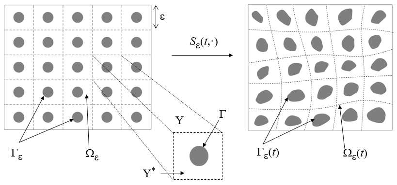
For $t\in[0,T]$, the evolving domain $\Omega_{\epsilon}(t)$ and the evolving surface $\Gamma_{\epsilon}(t)$ are described by a mapping $S_{\epsilon}:[0,T]\times\overline{\Omega}\to\mathbb{R}^{n}$,

with $\Gamma_{\epsilon}(t)=S_{\epsilon}(t,\Gamma_{\epsilon})$, see Figure 1. The Jacobi determinant of $S_{\epsilon}$ is denoted by $J_{\epsilon}$, i. e. we have $J_{\epsilon}:=\det\big(\nabla S_{\epsilon}\big)$.

Now we define the non-cylindrical domains $Q_{\epsilon}^{T}$ and $G_{\epsilon}^{T}$ by

and consider Problem P, namely to find $\tilde{u}_{\epsilon}$ satisfying:

Here, $\nu$ denotes the outer unit normal with respect to $\Omega_{\epsilon}(t)$, $\epsilon^{2}D$ is the diffusion-tensor, and $\epsilon\tilde{q}_{\epsilon}:\overline{\Omega_{\epsilon}}\to\mathbb{R}^{n}$ is a material velocity with the property that at the moving surface $\partial\Omega_{\epsilon}(t)$ it is equal to the evolution of the surface, $\epsilon\tilde{q}_{\epsilon}(t,\cdot)\cdot\nu=\partial_{t}S_{\epsilon}\big(t,S_{\epsilon}(t,\cdot)^{-1}\big)\cdot\nu$. We emphasize that this condition is needed for the derivation of the weak formulation of the problem, but not for the analysis. Therefore it is not stated in Assumption (AD1), referring to $\tilde{q}_{\epsilon}$. The functions $f$ and $\epsilon g$ describe the reaction kinetics in the bulk domain $\Omega_{\epsilon}(t)$, respectively at the surface $\Gamma_{\epsilon}(t)$. For more details about the derivation of such models we refer to e.g. [4].

We use common notations in the functional analysis. For a Banach space $X$ with norm $\|\cdot\|_{X}$ we also use this notation instead of $\|\cdot\|_{X^{n}}$ for the norm in the product space $X^{n}=X\times\ldots\times X$. Also, we use $C>0$ as a generic constant independent of $\epsilon$. With this, and assuming that all integrals are well defined, we obtain by integration by parts and the Reynolds transport theorem the following weak form of Problem P (as given in (1)):
Problem P_W. Find $\tilde{u}_{\epsilon}\in L^{2}((0,T),H^{1}(\Omega_{\epsilon}(t)))$ such that for all $\phi\in C^{1}\big(\overline{Q_{\epsilon}^{T}}\big)$ with $\phi(T,\cdot)=0$ it holds that

Below we state the assumptions on $S_{\epsilon}$:

1. (A1)

   $S_{\epsilon}\in C^{1}([0,T]\times\overline{\Omega_{\epsilon}})^{n}$ with

   $\displaystyle\frac{1}{\epsilon}\|\partial_{t}S_{\epsilon}\|_{C^{0}([0,T]\times\overline{\Omega_{\epsilon}})}+\|S_{\epsilon}\|_{C^{0}([0,T]\times\overline{\Omega_{\epsilon}})}+\|\nabla S_{\epsilon}\|_{C^{0}([0,T]\times\overline{\Omega_{\epsilon}})}$

   $\displaystyle\leq C.$

2. (A2)

   There exist constants $c_{0},C_{0}>0$ independently of $\epsilon$, such that

   $\displaystyle c_{0}\leq J_{\epsilon}\leq C_{0}.$

3. (A3)

   We have $J_{\epsilon}\in C^{1}([0,T]\times\overline{\Omega_{\epsilon}})$ with

   $\displaystyle\|\partial_{t}J_{\epsilon}\|_{L^{2}((0,T),\mathcal{H}_{\epsilon}^{\prime})}+\epsilon\|\nabla J_{\epsilon}\|_{L^{\infty}((0,T)\times\Omega_{\epsilon})}\leq C.$

   For the definition of the space $\mathcal{H}_{\epsilon}$ we refer to Section 3.

4. (A4)

   For any $\ell\in\mathbb{Z}^{n}$ with $|\epsilon l|<h$ and $0<h\ll 1$ fixed, it holds that

   	$\displaystyle\|J_{\epsilon}(\cdot_{t},\cdot_{x}+\ell\epsilon)-J_{\epsilon}\|_{C^{0}([0,T]\times\overline{\Omega_{\epsilon}^{h}})}$	$\displaystyle\leq C|\ell\epsilon|,\mbox{ and }$
   	$\displaystyle\|\nabla J_{\epsilon}(\cdot_{t},\cdot_{x}+\ell\epsilon)-\nabla J_{\epsilon}\|_{L^{\infty}((0,T)\times\Omega_{\epsilon}^{h})}$	$\displaystyle\leq C|\ell|,$

   For the definition of the domain $\Omega_{\epsilon}^{h}$ we refer to Section 3.

5. (A5)

   For any $\ell\in\mathbb{Z}^{n}$ it holds that

   $\displaystyle\|v_{\epsilon}(\cdot_{t},\cdot_{x}+\ell\epsilon)-v_{\epsilon}\|_{C^{0}([0,T]\times\overline{\Omega_{\epsilon}^{h}})}\leq C|\ell|\epsilon^{2},$

   with $v_{\epsilon}(t,x):=\nabla S_{\epsilon}(t,x)^{-1}\partial_{t}S_{\epsilon}(t,x)$ and $0<h\ll 1$ fixed.

6. (A6)

   There exists $S_{0}\in C^{0}\big(\overline{\Omega},C^{1}\big([0,T]\times\overline{Y^{\ast}}\big)\big)^{n}$ such that $S_{0}(t,x,\cdot_{y})$ is $Y$-periodic and $S_{0}(t,x,\cdot):Y^{\ast}\rightarrow Y(t,x):=\mathrm{R(S_{0}(t,x,\cdot))}$ (the range of $S_{0}(t,x,\cdot_{y})$) is a $C^{1}$-diffeomorphism and (for the definition of the two-scale convergence see Section 4)

   	$\displaystyle S_{\epsilon}(t,x)$	$\displaystyle\rightarrow x$	strongly in the two-scale sense,
   	$\displaystyle\nabla S_{\epsilon}(t,x)$	$\displaystyle\rightarrow\nabla_{y}S_{0}(t,x,y)$	strongly in the two-scale sense,
   	$\displaystyle\nabla S_{\epsilon}^{-1}(t,x)$	$\displaystyle\rightarrow\nabla_{y}S_{0}^{-1}(t,x,y)$	strongly in the two-scale sense,
   	$\displaystyle\epsilon^{-1}\partial_{t}S_{\epsilon}(t,x,y)$	$\displaystyle\rightarrow\partial_{t}S_{0}(t,x,y)$	strongly in the two-scale sense.

Especially, it holds that $J_{\epsilon}\rightarrow J_{0}:=\det\nabla_{y}S_{0}$ strongly in the two-scale sense. We emphasize that due to the estimates in Assumption (A1) the strong two-scale convergences in (A6) hold with respect to every $L^{p}$-norm for $p\in[1,\infty)$ arbitrary large. For the derivation of the macroscopic model we need the strong convergence of $\mathcal{T}_{\epsilon}J_{\epsilon}$, where $\mathcal{T}_{\epsilon}$ denotes the unfolding operator, see Section 4.

In the following we give an example of a transformation $S_{\epsilon}$, for which the assumptions (A1) - (A6) are fulfilled.

Finally, we state the assumptions on the data:

1. (AD1)

   It holds that $\tilde{q}_{\epsilon}\in L^{\infty}(Q_{\epsilon}^{T})^{n}$ and

   $\displaystyle\|\tilde{q}_{\epsilon}\|_{L^{\infty}(Q_{\epsilon}^{T})}\leq C.$

   Further, for $q_{\epsilon}(t,x):=\nabla S_{\epsilon}(t,x)^{-1}\tilde{q}_{\epsilon}(t,S_{\epsilon}(t,x))$ for almost every $(t,x)\in(0,T)\times\Omega_{\epsilon}$ we assume that for any $\ell\in\mathbb{Z}^{n}$ it holds that

   $\displaystyle\|q_{\epsilon}(\cdot_{t},\cdot_{x}+\ell\epsilon)-q_{\epsilon}\|_{L^{\infty}((0,T)\times\Omega_{\epsilon}^{h})}\leq C|\ell\epsilon|.$

   There exists a $Y$-periodic function $q_{0}\in L^{\infty}((0,T)\times\Omega\times Y^{\ast})$ such that

   $\displaystyle\tilde{q}_{\epsilon}\rightarrow\nabla_{y}S_{0}^{-1}q_{0}\quad\mbox{ in the two-scale sense,}$

   see Section 4 for the definition of two-scale convergence.

2. (AD2)

   It holds that $f,\,g\in L^{2}((0,T)\times\mathbb{R})$, and for almost every $t\in(0,T)$ the functions $z\mapsto f(t,z)$ and $z\mapsto g(t,z)$ are globally Lipschitz-continuous uniformly with respect to $t$.

3. (AD3)

   The diffusion tensor $D\in\mathbb{R}^{n\times n}$ is symmetric and positive.

4. (AD4)

   For $u_{\epsilon}^{0}(x)=\tilde{u}_{\epsilon}^{0}(S_{\epsilon}(0,x))$ it holds that $u_{\epsilon}^{0}\in L^{2}(\Omega_{\epsilon})$ are bounded uniformly with respect to $\epsilon$ and for any $\ell\in\mathbb{Z}^{n}$ such that $|\ell\epsilon|<h$ with $0<h\ll 1$ fixed, it holds that

   $\displaystyle\|u_{\epsilon}^{0}(\cdot+\ell\epsilon)-u_{\epsilon}^{0}\|_{L^{2}(\Omega_{\epsilon}^{h})}\overset{\ell\epsilon\to 0}{\longrightarrow}0.$

   Further, there exists $u^{0}\in L^{2}(\Omega\times Y^{\ast})$, such that $u_{\epsilon}^{0}\rightarrow u^{0}$ in the two-scale sense.

Using the mapping $S_{\epsilon}$, we transform the problem in (1) to the fixed domain $\Omega_{\epsilon}$. Let us define

and for $(t,x)\in(0,T)\times\Omega_{\epsilon}$

Then, by a change of coordinates, we transform Problem P_T into Problem P_T, which is defined on the fixed domain $\Omega_{\epsilon}$. We seek $u_{\epsilon}$ satisfying

In the following, given a bounded domain $U\subset\mathbb{R}^{n}$, the duality pairing between $H^{1}(U)^{\prime}$ and $H^{1}(U)$ is denoted by $\langle\cdot,\cdot\rangle_{U}$. With this we define a weak solution of Problem P_T (introduced in (3)):

The regularity of $\partial_{t}(J_{\epsilon}u_{\epsilon})$ and the regularity of $J_{\epsilon}$ immediately imply $\partial_{t}u_{\epsilon}\in L^{2}((0,T),H^{1}(\Omega_{\epsilon})^{\prime})$. However, as will be seen below the estimates for the norm of $\partial_{t}u_{\epsilon}$ are not uniform with respect to $\epsilon$, therefore we work with the product $J_{\epsilon}u_{\epsilon}$. We emphasize that in the variational equation (4) the time-derivative is applied to $J_{\epsilon}u_{\epsilon}$. This is unlike done Problem $P_{W}$, where the time derivative was applied to the test-function to avoid working with generalized time-derivatives for $\tilde{u}_{\epsilon}$ defined in Bochner-spaces with values in time-dependent function spaces. We emphasise that the analysis below is done for the transformed problem P_T.

We first introduce an $H^{1}(\Omega_{\epsilon})$-equivalent norm, which is more adapted to the $\epsilon$-scaling in the problem. We denote by $\mathcal{H}_{\epsilon}$ the space of $H^{1}(\Omega_{\epsilon})$ functions, equipped with the inner product

The associated norm is denoted by $\|\cdot\|_{\mathcal{H}_{\epsilon}}$. The spaces $H^{1}(\Omega_{\epsilon})$ and $\mathcal{H}_{\epsilon}$ are isomorphic with equivalent norms. More precisely,

We have the embedding

and for $F_{\epsilon}\in L^{2}((0,T),\mathcal{H}_{\epsilon}^{\prime})$ it holds that

Especially, for any $w_{\epsilon}\in L^{2}((0,T),\mathcal{H}_{\epsilon})\cap H^{1}((0,T),\mathcal{H}_{\epsilon}^{\prime})$ it holds that

Clearly, the converse embedding also holds: if $F_{\epsilon}\in L^{2}((0,T),H^{1}(\Omega_{\epsilon})^{\prime})$ then $F_{\epsilon}\in L^{2}((0,T),\mathcal{H}_{\epsilon}^{\prime})$ as well. However, in this case the estimates of the operator norms in the embedding depend badly on $\epsilon$,

We will see in Section 4 that the norm on $\mathcal{H}_{\epsilon}^{\prime}$ is the appropriate norm for the time-derivative to obtain two-scale compactness results.

The following Lemma provides some basic a priori estimates for the solution $u_{\epsilon}$ and the product $J_{\epsilon}u_{\epsilon}$.

We emphasize that in the proof above we used the $C^{1}$-regularity of $J_{\epsilon}$, but we have not assumed a uniform bound with respect to $\epsilon$ for the $C^{0}$-norm of the time-derivative $\partial_{t}J_{\epsilon}$. We overcome this problem by using the equality $\partial_{t}J_{\epsilon}=\nabla\cdot(J_{\epsilon}v_{\epsilon})$.

References

• [1] E. Acerbi, V. Chiadò, G. D. Maso, and D. Percivale. An extension theorem from connected sets, and homogenization in general periodic domains. Nonlinear Analysis, Theory, Methods & Applications, 18(5):481–496, 1992.
• [2] G. Allaire. Homogenization and two-scale convergence. SIAM J. Math. Anal., 23:1482–1518, 1992.
• [3] G. Allaire, A. Damlamian, and U. Hornung. Two-scale convergence on periodic surfaces and applications. in Proceedings of the International Conference on Mathematical Modelling of Flow Through Porous Media, A. Bourgeat et al., eds., World Scientific, Singapore, pages 15–25, 1996.
• [4] A. Alphonse, C. M. Elliott, and J. Terra. A coupled ligand-receptor bulk-surface system on a moving domain: well posedness, regularity, and convergence to equilibrium. SIAM Journal on Mathematical Analysis, 50(2):1544–1592, 2018.
• [5] T. Arbogast, J. Douglas, and U. Hornung. Derivation of the double porosity model of single phase flow via homogenization theory. SIAM J. Math. Anal., 27:823–836, 1990.
• [6] A. Bourgeat, S. Luckhaus, and A. Mikelić. Convergence of the homogenization process for a double-porosity model of immiscible two-phase flow. SIAM J. Math. Anal., 27:1520–1543, 1996.
• [7] C. Bringedal, I. Berre, I. S. Pop, and F. A. Radu. Upscaling of Non-isothermal Reactive Porous Media Flow with Changing Porosity. Transp. Porous Med., 114(2, SI):371–393, 2016.
• [8] C. Bringedal, L. von Wolff, and I. S. Pop. Phase field modeling of precipitation and dissolution processes in porous media: upscaling and numerical experiments. Multiscale Model. Simul., 18(2):1076–1112, 2020.
• [9] D. Cioranescu, A. Damlamian, P. Donato, G. Griso, and R. Zaki. The periodic unfolding method in domains with holes. SIAM J. Math. Anal., 44(2):718–760, 2012.
• [10] D. Cioranescu, A. Damlamian, and G. Griso. Periodic unfolding and homogenization. C. R. Acad. Sci. Paris Sér. 1, 335:99–104, 2002.
• [11] D. Cioranescu and A. Piatnitski. Homogenization of a porous medium with randomly pulsating microstructure. Multiscale Modeling & Simulation, 5(1):170–183, 2006.
• [12] D. Cioranescu and A. L. Piatnitski. Homogenization in perforated domains with rapidly pulsing perforations. ESAIM: Control, Optimisation and Calculus of Variations, 9:461–483, 2003.
• [13] M. Eden and A. Muntean. Homogenization of a fully coupled thermoelasticity problem for highly heterogeneous medium with a priori known phase transformations. Mathematical Methods in the Applied Sciences, 40:3955–3972, 2017.
• [14] M. Fotouhi and M. Yousefnezhad. Homogenization of a locally periodic time-dependent domain. Communications on Pure & Applied Analysis, 19(3):1669, 2020.
• [15] M. Gahn and M. Neuss-Radu. A characterization of relatively compact sets in Lp​(Ω,B)L^{p}(\Omega,B). Stud. Univ. Babeş-Bolyai Math., 61(3):279–290, 2016.
• [16] M. Gahn, M. Neuss-Radu, and P. Knabner. Derivation of an effective model for metabolic processes in living cells including substrate channeling. Vietnam J. Math., 45(1–2):265–293, 2016.
• [17] M. Gahn, M. Neuss-Radu, and P. Knabner. Homogenization of reaction–diffusion processes in a two-component porous medium with nonlinear flux conditions at the interface. SIAM J. Appl. Math., 76(5):1819–1843, 2016.
• [18] M. Gahn, M. Neuss-Radu, and P. Knabner. Effective interface conditions for processes through thin heterogeneous layers with nonlinear transmission at the microscopic bulk-layer interface. Networks and Heterogeneous Media, 13(4):609–640, 2018.
• [19] E. Hanzawa. Classical solutions of the Stefan problem. Tohoku Math. J., 33(3):297–335, 1981.
• [20] M. Lenczner. Homogénéisation d’un circuit électrique. Comptes Rendus de l’Académie des Sciences-Series IIB-Mechanics-Physics-Chemistry-Astronomy, 324(9):537–542, 1997.
• [21] J. E. Marsden and T. J. R. Hughes. Mathematical Foundations of Elasticity. DOVER PUBN INC, 1994.
• [22] A. Meirmanov and R. Zimin. Compactness result for periodic structures and its application to the homogenization of a diffusion-convection equation. Elec. J. of Diff. Equat., 115:1–11, 2011.
• [23] A. Mielke, S. Reichelt, and M. Thomas. Two-scale homogenization of nonlinear reaction-diffusion systems with slow diffusion. Networks & Heterogeneous Media, 9(2):353 – 382, 2014.
• [24] T. Muthukumar, J.-P. Raymond, and K. Sankar. Homogenization of parabolic equation in an evolving domain with an oscillating boundary. Journal of Mathematical Analysis and Applications, 463(2):838–868, 2018.
• [25] M. Neuss-Radu. Some extensions of two-scale convergence. C. R. Acad. Sci. Paris Sér. I Math., 322:899–904, 1996.
• [26] M. Neuss-Radu and W. Jäger. Effective transmission conditions for reaction-diffusion processes in domains separated by an interface. SIAM J. Math. Anal., 39:687–720, 2007.
• [27] G. Nguetseng. A general convergence result for a functional related to the theory of homogenization. SIAM J. Math. Anal., 20:608–623, 1989.
• [28] M. A. Peter. Homogenisation in domains with evolving microstructures. C. R. Macanique, 335:357–362, 2007.
• [29] M. A. Peter. Coupled reaction–diffusion processes inducing an evolution of the microstructure: Analysis and homogenization. Nonlinear Analysis: Theory, Methods & Applications, 70(2):806 – 821, 2009.
• [30] M. A. Peter and M. Böhm. Multiscale modelling of chemical degradation mechanisms in porous media with evolving microstructure. Multiscale Modeling & Simulation, 7(4):1643–1668, 2009.
• [31] J. Prüss and G. Simonett. Moving Interfaces and Quasilinear Parabolic Evolution Equations. Birkhäuser, 2016.
• [32] M. Redeker, C. Rohde, and I. S. Pop. Upscaling of a tri-phase phase-field model for precipitation in porous media. IMA J. Appl. Math., 81(5):898–939, 2016.
• [33] I. E. Scheffler. Mitochondria. John Wiley & Sons, 2008.
• [34] R. Schulz and P. Knabner. Derivation and analysis of an effective model for biofilm growth in evolving porous media. Math. Methods Appl. Sci., 40(8):2930–2948, 2017.
• [35] R. Schulz, N. Ray, F. Frank, H. S. Mahato, and P. Knabner. Strong solvability up to clogging of an effective diffusion-precipitation model in an evolving porous medium. Euro. Jnl of Applied Mathematics, 2016.
• [36] J. Simon. Compact sets in the space Lp​(0,T,B){L}^{p}(0,{T};{B}). Ann. Mat. Pura Appl., 146:65–96, 1987.
• [37] T. L. van Noorden. Crystal precipitation and dissolution in a porous medium: Effective equations and numerical experiments. Multiscale Modeling & Simulation, 7(3):1220–1236, 2009.
• [38] T. L. van Noorden and A. Muntean. Homogenisation of a locally periodic medium with areas of low and high diffusitvity. Euro. Jnl of Applied Mathematics, 22:493 – 516, 2011.
• [39] T. L. van Noorden and A. Muntean. Corrector estimates for the homogenization of a locally periodic medium with areas of low and high diffusivity. Euro. Jnl of Applied Mathematics, 24:657 – 677, 2013.
• [40] C. Vogt. A homogenization theorem leading to a volterra integro-differential equation for permeation chromotography. SFB 123, University of Heidelberg, Preprint 155 and Diploma-thesis, 1982.