Calabi-Yau threefolds with Picard number three
Abstract.
In this paper, we continue the study of boundedness questions for (simply connected) smooth Calabi–Yau threefolds commenced in [6]. The diffeomorphism class of such a threefold is known to be determined up to finitely many possibilities by the integral middle cohomology and two integral forms on the integral second cohomology, namely the cubic cup-product form and the linear form given by cup-product with the second chern class. The question addressed in both papers is whether knowledge of these cubic and linear forms determines the threefold up to finitely many families, that is the moduli of such threefolds is bounded. If this is true, then in particular the middle integral cohomology would be bounded by knowing these two forms.
Crucial to this question is the study of rigid non-movable surfaces on the threefold, which are the irreducible surfaces that deform with any small deformation of the complex structure of the threefold but for which no multiple moves on the threefold. We showed in [6] that if there are no such surfaces, then the answer to the above question is yes. Moreover if , the answer was shown to be yes without the further assumption on the Calabi–Yau.
The main results of this paper are for Picard number , where we prove boundedness
in the case where there is at most one rigid non-movable surface, assuming the cubic form is smooth, thereby defining a real elliptic curve; in the two cases where the Hessian curve is singular, we also assume that
the line defined by the second chern class does not intersect this curve at an inflexion point. The arguments
used nicely illustrate the general theory developed by the author in the first half of [6].
In addition to the methods described in [6], a further crucial tool in the proofs will be the classical Steinian involution on the Hessian of an elliptic curve.
2000 AMS Subject Classification: Primary 14J32, Secondary 14J30, 14J10
Keywords: Calabi–Yau threefolds. Birational classification. Boundedness of families.
Introduction
Throughout this paper, will denote a (simply connected) smooth complex Calabi–Yau threefold. We know that its diffeomorphism class is determined up to finitely many possibilities by knowledge of the cup-product cubic form on given by , the linear form on given by and the middle cohomology [3, 4]. A well-known question is whether the Calabi–Yau threefold is determined up to finitely many families by the diffeomorphism type. In the paper [6], we addressed the question as to whether is determined up to finitely many families by the weaker information of the cubic and linear forms on , and in particular proved this was true for Picard number . In this paper we start the study of higher Picard number. We saw in [6] that the rigid non-movable surfaces played a central role in this question; if there are no such surfaces on , then boundedness was proved in general for all .
Following definitions from [6], the positive index cone of the cubic is the set of classes for which and the quadratic form given by has index . Recall that if is the component of the positive index cone on a Calabi–Yau threefold which contains the Kähler cone , we consider the subcone of given by the extra conditions that for all rigid non-movable surfaces on , and let be the component of this cone which contains the Kähler cone. Assuming that there are only finitely many such surfaces and that is general in moduli, we showed in [6] that any integral class in will have for some (Proposition 4.1 and Lemma 4.3), with explicitly dependent on the class; in particular for a movable class and supported on the rigid non-movable surfaces. Recall that a class is said to be movable if it is in the closure of the cone generated by mobile classes, where an integral class is called mobile if it corresponds to a non-empty linear system with no fixed component. The cone of movable classes is called the movable cone .
The main results of this paper are for Picard number . A crucial tool in the proofs will the classical Steinian involution on the Hessian of a real elliptic curve. We recall below that there are only two possibilities where the Hessian of the elliptic curve is singular, and in both these special cases the real elliptic curve has one real component.
Main Theorem.
Suppose is a Calabi–Yau threefold with Picard number for which the cup-product cubic form and the linear form defined by the second chern class on are specified, and where the corresponding plane cubic curve is smooth. Assume contains at most one rigid non-movable surface.
(i) If the above real elliptic curve has two components, then the Kähler cone of is contained in the positive cone on the bounded component; moreover lies in a bounded family.
(ii) If the real elliptic curve has one component and the Hessian curve is smooth, then there is a rigid non-movable surface on and its class lies in the closed half-cone on which determined by the bounded component of the Hessian; moreover lies in a bounded family.
(iii) If the Hessian curve is singular and the line in does not intersect the elliptic curve at an inflexion point, then contains a rigid non-movable surface and lies in a bounded family.
Corollary.
If is a Calabi–Yau threefold with Picard number for which we have specified the above cubic and linear forms on , where the corresponding cubic curve and its Hessian are smooth, then for sufficiently large there must be at least two rigid non-movable surfaces on . If the Hessian curve is singular, we have the same result provided we assume also that the line does not intersect the real elliptic curve at an inflexion point.
Let me indicate one of the main ideas we shall need. We will say that a non-zero point on the boundary of a convex cone is visible from a point if the line segment joining and does not meet the interior of . If is a smooth point of , the tangent hyperplane through determines a closed half-space whose intersection with the interior of is empty; then is visible from if and only if is in this half-space. The set of points in which are visible from and will be called the visible extremity of from ; a non-zero smooth point is in the visible extremity from if and only if is in the tangent hyperplane. A non-zero which is not in the visible extremity from will not be visible from if and only if it is visible from , and also if and only if is visible from with respect to . A guiding result is the following:
Proposition 0.1.
Let be a Calabi–Yau threefold containing finitely many rigid non-movable surfaces , with is the component of the positive index cone which contains the Kähler cone; consider the open subcone of given by the conditions for all and let be the component containing the Kähler cone. Any point of the boundary of at which the cubic form is positive and the Hessian form vanishes, but which is not visible from any of the , must be big.
Proof.
We may assume that is general in moduli, and then the elements of the pseodoeffective cone are those of the form , for a real movable divisor and non-negative real numbers. As commented above, since the Kähler cone is a subset of , any element of is of such a form, and so its closure . The claim is that is big.
Suppose to the contrary that lies in the boundary of . Since it is not visible from any of the classes with respect to , it is not visible from any of the classes with respect to the convex cone . It follows that the real numbers defined above above must all be zero, and so ; in fact must lie in its boundary. We saw in the second proof of Theorem 0.1 in Section 4 of [6] that for any movable class , we have . Thus and so was big after all. ∎
Remark 0.2.
Let us comment how this result will be used. Assuming is general in moduli, we know that , for some real movable divisor and some real effective class . In the cases we study, we shall show that but it is in (the closure of) a different component of the positive index cone. If denotes an ample class on , then is big and movable for all and hence the Hessian is always non-negative on the line segment from to ; by varying a little we’ll see that the Hessian may be assumed strictly positive on this line segment, apart maybe at itself. As however for all , we deduce from connectedness that lies in , which will be the required contradiction.
In particular, assuming there are no rigid non-movable surfaces on , we suppose that denotes the component of the positive index cone containing the Kähler cone. If is general in moduli, then not only will but also any big class will be movable, and in particular has non-negative Hessian. Thus Proposition 0.1 implies that there are no points on the boundary of at which the cubic is positive and at which the Hessian is smooth and vanishes, since otherwise there would be nearby rational points which were both big and had strictly negative Hessian. In the case therefore when when the cubic hypersurface is smooth, this recovers the fact that under the above assumptions, the hypersurface must have two components, and the Kähler cone on is contained in the positive (open) cone on the bounded component ([6], Remark 4.7), which in turn is contained in the strictly movable cone , namely the interior of . Thus any integral in the positive cone on the bounded component is big and movable.
In the case , we noted that there are at most two rigid non-movable surfaces, and the more delicate case was when there were precisely two — the case of one such surface was slightly easier. In this paper we shall mainly be considering the case for higher Picard number where there is precisely one rigid non-movable surface on . In this case we have a strengthening of a result from [6] — cf. Lemma 5.4 there. In the case of and the cubic is smooth, we deduce that can only happen if represents an inflexion point of the elliptic curve.
Lemma 0.3.
For arbitrary , let denote the closure of the component of the positive index cone that contains the Kähler cone and be the class of the unique rigid non-movable surface on ; if , then the cubic form and its Hessian together with the linear form must all vanish at .
Proof.
Given such an , we would have for all by Lemma 3.3 of [6]. From the same lemma, we have for all . (If for some , then for any we have for and hence for any ; this in turn implies that and so the Hessian would vanish at .) So in particular the open subcone of defined by is the whole of . By Proposition 4.4 of the same paper, the assumptions imply that and , since otherwise some multiple of would move. A major part of the proof of Lemma 5.4 of [6] was that for any there then exists a mobile big divisor with . In our case therefore, represents a smooth point of the cubic form; moreover and are on different sides of the tangent hyperplane given by . If now the Hessian does not vanish at , then for small , we have , since for . However, we know then that for some movable class and real . Thus some multiple of is movable and big; clearly a negative multiple of cannot be effective, and so we deduce that is movable, a contradiction. ∎
Throughout this paper, we may without loss of generality take to be general in moduli; recall from [5] that the Kähler cone is essentially invariant under deformations and it is always contained in the Kähler cone of a general deformation.
The overall plan of the paper is as follows. In Section 1, we describe explicitly the components of the positive index cone associated to a smooth ternary cubic. We will then consider the case when the cubic comes from the cup-product on for a Calabi–Yau threefold with Picard number . For the case when the corresponding real elliptic curve has two components, and is a rigid non-movable surface on , we employ the Steinian involution in Section 2 to describe the open subcone defined by the quadratic inequality for any component of the positive index cone. This enables us in this case to deduce that, when contains at most one rigid non-movable surface, the Kähler cone must be contained in the positive cone on the bounded component of the elliptic curve. We use this in Section 3 to prove boundedness in this case. Finally in Section 4, we employ the Steinian involution to study in more detail the case when the real elliptic curve has one component. Under the assumption that there is at most one rigid non-movable surface on , this can occur only for a smooth Hessian when lies in the closed half-cone on which determined by the bounded component of the Hessian, or in one of the two cases where the Hessian is a singular curve, and in all these cases we can deduce boundedness, in the latter two cases under the mild extra condition that the line does not contain an inflexion point of the curve.
1. Components of the positive index cone for real ternary cubics
In [6], a central role was played by the positive index cone corresponding to the cubic, namely the classes for which and the quadratic form given by has index . For the cubic defines a curve in the real projective plane, and this is the main case we shall study in this paper. In this paper, we shall not study the case when the cubic curve is singular, which would involve case by case arguments, and our initial aim will be to understand the positive index cone in the smooth case. To study real elliptic curves, the Hesse normal form for the curve will be useful, the theory of which may be found in [1] or Section 3 of [2]. Normally we might take real coordinates so that the real elliptic curve takes Hesse normal form , but for our purposes it will be more convenient to make a change of coordinates so that the cubic takes the form
so that the ‘triangle of reference’ of is now in the affine plane with vertices and . We shall write if we wish to indicate the dependence on . Recall that if , then the real curve has two components, the bounded component (lying in the triangle of reference) and the unbounded component. The cone in corresponding to the bounded component has two components when one removes the origin, a positive part inside which and a negative part inside which , whilst the cone on the unbounded component only has one component in , even after removing the origin. In the case it is easily checked that the unbounded component has three affine branches, one of which lies in the negative quadrant , one in the sector and the third in the sector . The inflexion points of the cubic are at and , i.e. the intersection of the line at infinity with the curve (a further reason why the chosen change of coordinates is helpful). The asymptotes for the affine branches of the unbounded component may be found by calculating the tangents to the curve at the inflexion points, and are
Noting that , where is a primitive cube root of unity, when the cubic (1) splits into the real line and two complex lines (meeting at the centroid of the triangle of reference.
When , the cubic is smooth but with only one real component, with three affine branches, one in the region , one in the region and one in the region . The asymptotes are calculated as before and are given by the equations (2). The case is special, partly because it is the only smooth case where the asymptotes are concurrent, with the common point being the centroid of the triangle of reference.
If one calculates the Hessian form of the cubic , one obtains
Thus if denotes the Hessian of the cubic , the fact that our change of coordinates was unimodular shows for that , with constant . In particular we see that if , then , and so the Hessian curve of a real elliptic curve with two components has only one component. For , we have two notable values: for which the Hessian is the three real lines given by , and for which the Hessian curve is the three lines (two of them complex) corresponding to described before. Apart from these two values, for any real elliptic curve with one component, the Hessian is a real elliptic curve with two components, the bounded component lying in the triangle of reference.
The case of the curve having two components is illustrated in Figure 1 (which shows , and the three asymptotes for ). The picture for one component when is not dissimilar, where the roles of the cubic and its Hessian are switched. For or , we note that the asymptotes to the cubic are tangent to the affine Hessian curve ; this is just a special case of a classical result that the double polar with respect to the cubic at a point on its Hessian is tangent to the Hessian at the image of the point under the Steinian involution (see [2], Section 3.2 and Exercise 3.8). When the point is an inflexion point of the cubic, the double polar is just the tangent line to the cubic, in our case the asymptote — the corresponding points on the Hessian are labelled , . This gives more precise information about the affine regions where the Hessian curve can lie.

We now identify the components of the positive index cone. Taking the affine piece of a real cubic as above, one looks for the regions for which either and , or and , the latter being relevant since for in such a region, both and will be positive at . In order to keep track of signs, we note that for all and that for . Moreover the index of the quadratic form is at .
If has two real components, i.e. , then the curve bounds precisely four (convex) regions of the affine plane on which both and . On these regions, we note that the index of the corresponding quadratic form is . Moreover the Hessian curve bounds precisely three (convex) regions of the affine plane on which both and are negative (where the index of the associated quadratic form is ). Apart from the bounded component inside which (contained in the triangle of reference), each unbounded component defined by will together with the negative of the appropriate region defined by give rise to a connected component of the positive index cone in , part of whose boundary is contained in and part of whose boundary is contained in , with the two parts meeting along rays corresponding to two of the inflexion points of the curve . For each of these three resulting hybrid cones in , we have and a continuity argument verifies that the index is on each cone. The other component of the positive index cone corresponds to the bounded component and whose boundary is contained in .
In the case when only has one connected component, i.e. , we have that the condition defines three (convex) regions of the affine plane . There are two special cases here, when and . For all other values of , there are four components of the positive index cone. Three are hybrid, obtained from unbounded affine regions on which together with the (negative of) unbounded affine regions on which ; a continuity argument again ensures that the index is . The remaining component corresponds affinely to the bounded component of ; on the corresponding open half-cone we have , and the index is — this latter claim can be checked in a number of ways (one way is to check it for points in the triangle of reference for the Fermat cubic and using a continuity argument, since as the bounded component of the Hessian of tends to this triangle). Thus points in the negative of the corresponding cone have index as required, to give a connected component of the positive index cone.
In the special case , the Hessian is ; again there will be three hybrid components of the positive index cone, each bounded by the cone on one of the affine branches of and two linear parts corresponding to segments of two of the three lines of the Hessian. As in the general case, there is also the negative cone on the bounded component of the Hessian, in this case corresponding to the whole triangle of reference. The other special case is when : here we have on all the affine plane except at the point , and the positive index cone has just the three connected components, each bounded by the (positive) cone on an affine branch of the curve and a cone in the plane corresponding to the line at infinity, the real component of the curve . Here the bounded component of has shrunk to a point, and so does not contribute to the components of the positive index cone.
In both cases, namely the real elliptic curve has one or two components, the components of the positive index cone are all convex, and their closures are strictly convex unless .
Notation.
We shall now fix on the notation that will be used in the rest of this paper to describe a hybrid component of the positive index cone. Taking the affine slice , where the cubic is of the form described above, with slight abuse of notation concerning the points at infinity, we denote the projectivised boundary of by , where is an affine branch of and is an associated affine branch of , with and meeting at two inflexion points (at infinity). When , without loss of generality we may take in the negative quadrant and then in the region . The branches and meet (at infinity) at the inflexion points and . More specifically, the closed component then has boundary the positive cone on together with the negative cone on , the two parts meeting in two rays corresponding to positive multiples of and ). When and , we take in the region and in the negative quadrant. The branches and again meet (at infinity) at the inflexion points and . The component then has boundary the positive cone on together with the negative cone on , the two parts meeting in the two rays corresponding to positive multiples of and ). For , the only change is to take to denote the union of the two line segments and in the affine plane . For , we shall take to denote the line segment at infinity from to . The boundary of in this case is the positive cone on together with the cone generated by and in
Proposition 1.1.
Suppose is a Calabi–Yau threefold with Picard number and there is at most one rigid non-movable surface on . If the cubic form defines an elliptic curve with one real component, for which the Hessian has a non-trivial real bounded component (i.e. in the notation above, when and ), then the Kähler cone of is not contained in the component of the positive index cone corresponding to the bounded component of the Hessian.
Proof.
We suppose the contrary, so that then the convex cone by index considerations. We observed that the result is true if there are no rigid non-movable surfaces on . We may assume that is general in moduli and there is a unique such surface . We then choose in the boundary of the convex cone which is not visible from . Since for all movable classes , we deduce that , and hence is big. We write for some suitable real movable class and , and thus . By convexity for all since is not visible from , hence a contradiction. ∎
For a Calabi–Yau threefold with Picard number where there is at most one rigid non-movable surface on , Sections 2 and 4 will rule out the possibility of the Kähler cone being contained in a hybrid component of the positive index cone (except for some special cases when the real elliptic curve has one component, for which cases we can prove boundedness results), where hybrid by definition means that part of the boundary consists of points where vanishes and part where vanishes, as described above. This then reduces us down in Section 3 to considering the case where the elliptic curve has two components and the Kähler cone is contained in the positive cone on its bounded component, for which case we can also prove boundedness (Corollary 3.8).
We note that if is a point in the open arc of rays in the boundary of as specified in the statement of the following Proposition, then a line segment from to the given class contains interior points of if and only if it contains interior points of . So in this case we can talk about being visible or not visible from without specifying whether we consider to be on the boundary of or , or indeed say the negative cone on the interior of .
Proposition 1.2.
Suppose is a Calabi–Yau threefold with Picard number for which the cubic form defines a smooth elliptic curve, and that contains a unique rigid non-movable surface . Let denote a component of the positive index cone and a component of the open subcone of given by . If the boundary of contains a non-empty open arc of rays which are not visible from but on which the Hessian vanishes and the cubic form is strictly positive, then does not contain the Kähler cone.
Proof.
As usual, we may assume that is general in moduli. In the light of Proposition 1.1, we may assume to be a hybrid component of the positive index cone; we assume that contains the Kähler cone and obtain a contradiction. Let be any point in one of the specified rays in the boundary; Proposition 0.1 then implies that for some , the class is movable. Moreover, the argument from the proof of Proposition 1.1 shows that is not movable and . With the notation from this section, we may take . Let us assume first that we are not in either of the two special cases or — the argument will in fact be very similar in these cases.
We then have the possibilities that either some real multiple of represents a point of the affine plane , or represents a point on the line at infinity . Suppose first that is a negative multiple of , and so . Then the point is not visible with respect to the cone from the point , and in particular the line segment from to cuts the Hessian curve at points , and one other point; note here that we are using from Lemma 0.3. Consider now ; if this were to lie in the half-plane , then we would have , a contradiction. Thus lies in the half-plane , and so , showing that is in the closure of a different component of the positive index cone.
The next possibility is that is a positive multiple of ; then is visible from ; moreover by Proposition 0.1 we have such that is movable, and hence for some that is movable. Now consider the line segment consisting of points for ; since , the Hessian will vanish when and precisely one more point. We deduce therefore that at we have and , so that is in (the closure of) a different component of the positive index cone.
Finally, if represents a point on the line at infinity, we know from Lemma 0.3 that either represents one of the two inflexion points at infinity on (noting that the sign is determined since for any ample class ), or . In the first case, since and , we see from the geometry of the affine curves that is in (the closure of) a different component of the positive index cone. If represents the third inflexion point (and so ), then we must have ; the fact that is visible from implies (again from the affine geometry) that for all , contradicting the fact it is non-positive for . The remaining possibility is that lies in the interior of the cones on the other two line segments with on which (since we know that ). The fact that the chosen class is visible from implies that it is visible from with respect to the cone on , and the affine geometry then again yields that for all , contradicting the fact it is non-positive for .
In all possible cases therefore, is in (the closure of) a different component of the positive index cone, and so in particular , and we obtain a contradiction via the argument in Remark 0.2.
The reader is invited to check that the same arguments hold true in the case when as for the general case when ; the ability to perturb ensures that in the case where the movable divisor is in the closure of another component of the positive index cone, it is not also in . For , it is even more straightforward; in this case if and only if is a point of the affine plane and not the singular point. We know also that the open arc specified in the Proposition corresponds to an open interval of the line segment at infinity, i.e all its points lie in the cone generated by and . We have seen in Lemma 0.2 that unless it is one of the points at infinity on , and since for any ample , it follows from Lemma 3.3 of [6] that . Moreover, if were to lie on the line at infinity, then any choice of in the open arc specified would be visible from . The assumptions of the Proposition therefore ensure that is a positive multiple of a point in the affine plane , and given we may perturb our choice of if required so that the Hessian is non-singular at all points on the line through and ; hence the Hessian takes negative values on for all ; thus is not movable for any , contradicting the conclusion of Proposition 0.1. ∎
2. Steinian map when elliptic curve has two real components
With notation as in the previous section, we let denote a component of the positive index cone, with closure . The next piece of the jigsaw puzzle will be to understand the function , where and , and in particular where it vanishes on the affine slice of the boundary of a component of the positive index cone. In this section, we study the case when , i.e. the real elliptic curve has two components.
The component of the positive index cone which corresponds to the bounded component of is then easy to understand; phrasing things affinely, we know that for on the bounded component is just saying that lies on the tangent to the curve at . Assuming that corresponds to a point outside the bounded component, the conic intersects that boundary of the component precisely at the points where the tangent to the curve passes through , and hence corresponds to the boundary of the visible points from (where we recall visible here means the points on the bounded component for which the closed line segment does not include any points inside the component); we used the term visible extremity for the set of such points.
We therefore need to understand the hybrid components . Here we adopt the notation from Section 1. In view of Lemma 0.3, we assume ; as above there is then a simple answer to the question of where on we have vanishing of , namely points on of for which the tangent passes through (including maybe inflexion points at infinity). There will be two such points if is in the quadrant (including the possibilities of the inflexion points and ), no such points if is in the quadrant and one point otherwise. Let us consider the branch of the Hessian passing through and , the affine point with coordinates . As is the third inflexion point, we have already observed that the tangent to at is tangent to at , i.e. that if we take to be the zero of the group law, then is the unique real 2-torsion point of the Hessian. Recall the classical fact that there is a well-defined base-point free involution on the Hessian curve, known as the Steinian involution ([2], Section 3.2, noting a misprint in Corollary 3.2.5), where the polar conic of with respect to a point on is a line pair with singularity at . In the case currently under consideration where the Hessian has only one real component, corresponding to a choice of inflexion point for the zero of the group law, there is a unique real 2-torsion point, and is given by translation in the group law by this point. The Steinian map has the property that for any point , the second polar of with respect to the point is the tangent to the Hessian at ([2], Exercise 3.8, noting a misprint). Let be the point on the branch of in the region , which is the 2-torsion point when we take as the zero in the group law, the point on the branch of in the region corresponding to , and the point on the branch of in the region corresponding to . It is left to the reader to check that , and . Thus the second polar of with respect to the inflexion point is the tangent to the Hessian at , namely given affinely by , the second polar of with respect to the inflexion point is the tangent to the Hessian at , namely given affinely by , and the second polar of with respect to the point is the tangent to the Hessian at , namely the asymptote , where as defined before.
Setting , it is easily checked from this that iff , that iff and that iff . Moreover if , then for and if then . We are interested in the cases of and since we want to know the sign of on points of where either or . This gives us a dictionary as to how many points of there are at which the function vanishes.
Lemma 2.1.
Suppose and . If , so that , then vanishes precisely once on the interior of the open arc of , and does not vanish on the interior of the open arc . If , then vanishes once on the interior of the arc and twice at , and is non-vanishing on the open arc . If , so that , and lies in the open region between the arc of the Hessian from to , the line and the line , then will vanish precisely twice on the open arc and once on the open arc . If lies on the arc of the Hessian from to , then is a line pair whose singularity lies in the interior of the arc of , one line of the pair also intersecting and the other line also intersecting at some point in the interior of the arc . For the remaining points satisfying the initial inequalities, is non-vanishing on the arc and has one zero on the interior of the arc of .
Proof.
Note that the second polar of a point in the arc of from to corresponds to the tangent line to the Hessian at on the arc of the Hessian going from to . Furthermore we note that for a given point , we are asking how many points on the arc of the Hessian from to , the tangent at contains . We note that is clearly on no such tangent line if is strictly below the arc of the Hessian going from to , and if lies on this arc, the answer is one (as the relevant tangent line is just the tangent to the Hessian at ). In this case is a line pair with singularity at as claimed. From the geometry we see that also lies on a tangent line at a point of the Hessian arc and also on a tangent line of ; this then gives the required statements in this case. If is strictly above the arc , then the claims are clear geometrically since we are looking for points of the visible extremity of the convex set with boundary the affine branch of the Hessian as seen from , lying on the arc of the Hessian from to , and there will be one such point unless lies in the open region specified in the statement of the Lemma, in which case there are two. The remaining claims of the lemma are also clear from the geometry, since we are additionally asking if there are points on the open arc of the Hessian, the tangent line at which passes through .∎
By symmetry, we have a corresponding result for and . We can then deduce the following result.
Corollary 2.2.
If and , then vanishes twice on the closed arc (including possibly the inflexion points in the case of an equality), and not at all on the affine branch . If and then is non-zero on the closed arc ; in this case if , then will also be non-zero on the arc , and if it will vanish twice on (in the case of equality, twice at the point ). In all other cases, will intersect (the closure of) precisely once and the affine arc either once or three times
Summing up therefore, the conic either intersects the projectivised boundary of twice (including the case when it is the point with multiplicity two), or four times in the cases specified. Since we know that is convex, we know in particular that the cone is connected when we just have the two points of intersection, but will have two components when there are four (distinct) intersection points. If the index at is with , it follows from Proposition 3.4 of [6] that any component of the above cone is also convex. If has index , then has index , and the cone is convex. If however lies on the affine arc of the Hessian from to , the second polar with respect to is a line pair with a singularity at the corresponding point of , as detailed in Lemma 2.1. The open cone then has two (convex) components, and the open cone has one (convex) component, reflecting the fact that if the index at is , then that is also the index at .
Proposition 2.3.
Suppose is in the affine plane with , . If , then any component of contains an open arc of points visible from . In the case of , some open arc in is not visible from .
Proof.
Since , we have that intersects precisely once on the open arc if , and in this case . The condition defines a convex subcone of containing , part of whose boundary corresesponds to an arc of in (namely the part near ), which is visible from . If , then we may have or . If , then the condition defines a subcone of containing , and part of the boundary of one component corresponds to an arc in , part of which (namely the part near ) is visible from . If the above subcone contains a second component, then part of its boundary corresponds to a second arc in whose interior contains , and so part of that arc is also visible from . If , then the condition defines a convex subcone of containing , part of whose boundary corresponds to an arc of in , part of which (namely the part near ) is not visible from .∎

Before proceeding further, the reader might find Figures 2 and 3 helpful. We are taking as in Figure 1, and is the branch of the Hessian in the positive quadrant. In both figures, the point is marked, is the hybrid component of the positive index cone with boundary corresponding to , and the areas corresponding to the subcone have been shaded. For Figure 2 we take to be the affine point ; here and so by Proposition 2.3, we have part of is visible from . The picture when lies in the open region between the arc of the Hessian and its asymptote is similar to Figure 2, except that has two possible components, with one having part of its boundary corresponding to an open arc of containing , part of which is visible from . For Figure 3 we take , so that and part of is not be visible from .

Proposition 2.4.
If is a Calabi–Yau threefold with Picard number whose corresponding real cubic curve is smooth with two real components, and there is at most one rigid non-movable surface on , then the Kähler cone must be contained in the positive cone on the bounded component of the elliptic curve.
Proof.
The content of this result is that the Kähler cone cannot be contained in a hybrid component of the positive index cone. We already know this in the case of no such surfaces, so suppose we have a unique such surface . We suppose that the result is not true, so that the Kähler cone is contained in a hybrid component , which we may assume to be bounded by and , with the notation as before. The index of at the point is for . We let denote the convex cone .
Claim.
There is an arc of points on , the negative multiples of which correspond to rays as specified in the statement of Proposition 1.2.
Assuming does not lie on the line at infinity , we let denote the intersection of the line though with the affine plane . Suppose the Kähler cone is contained in a hybrid , which without loss of generality we may take to comprise of the (positive) cone on interior of the affine branch of together with the negative cone on the interior of the affine branch of , the two parts meeting along the cone spanned by and .
If is such that does not properly intersect either or , namely with and , then is negative on the whole cone , which contradicts containing the Kähler cone, since in this case we note that the index of is and so is a positive multiple of . If is such that intersects twice (possibly including points at infinity), then we check easily that the boundary of contains the whole negative cone on . In this case we also note that the index of is and so is a positive multiple of . Since all of is visible from the affine point , none of the negative cone on may be seen from , and so the corresponding points of the boundary of may not be seen from , and the Claim is proved.
If now vanishes twice on (namely and ), then (which is negative at and ) will be positive on a region inside of with boundary including the arc of between the two intersection points. Such a point is also a positive multiple of . Points of this arc may plainly be seen from , and so the corresponding points of the boundary of may not be seen from , and the Claim follows.
We are left with the case where is as in Proposition 2.3, or by symmetry where the roles of and are switched. The Claim then follows from this previous result.
Finally we should mention the case when lies on the line at infinity. We know that by Lemma 0.3, unless represents one of the inflexion points or . In this latter case on , and so there is no difficulty finding an arc of rays in the boundary of which are not visible from . If represents the inflexion point , then touches the boundary of along two rays, corresponding to and the symmetry point on . Thus the subcone is either empty or the whole of , in which latter case the claim is true since half of the cone on is visible from and half is not. The other case is when ; knowing that , we have that , where either or , where by symmetry we may assume the former case. In this case, the same argument says that is positive on an arc of (namely from to the point on the arc where vanishes), which points are visible from and again the Claim follows.
Thus we merely need to combine the Claim with Proposition 1.2 to deduce that the Kähler cone cannot be contained in a hybrid component of the positive index cone, and so it must be contained in the positive cone on the bounded component of the elliptic curve. ∎
3. Boundedness when elliptic curve has two real components
The result of Proposition 2.4 extends to give a corresponding result for any . Note however that the cubic having two real components in higher dimensions is a stronger condition; for smooth cubic surfaces for instance, it is well-known that there are five real diffeomorphism types and only one of these has two components.
Theorem 3.1.
Let be a Calabi–Yau threefold which is general in moduli with Picard number whose corresponding cubic hypersurface is smooth with two real components. If there is at most one rigid non-movable surface on , then the Kähler cone must be contained in the positive cone on the bounded component of the cubic hypersurface.
Proof.
We choose a general ample integral class and a general integral class inside the positive cone on the bounded component of the cubic hypersurface, and we take the 3-dimensional slice of through the origin and the classes , and . We therefore obtain a cone on a smooth elliptic curve with two real components, defined by the restriction of the cubic form to . Unless , the Hessian of the elliptic curve is not of course the restriction of the Hessian hypersurface to (if only since the degrees are different). If , then the quadratic form on associated with a non-trivial divisor has index or , according to whether the Hessian of the (smooth) restricted cubic is positive, negative or vanishes. It will turn out that the Hessian of the restricted cubic plays a more crucial role than the restriction of the original Hessian.
We suppose that the Kähler cone is not contained in the positive cone on the bounded component, and so is not contained in the positive cone on the bounded component of the elliptic curve; we suppose that is contained in some other component of the positive index cone of the elliptic curve — the restriction of the component of the positive index cone of the cubic on containing is an open subcone of . We let denote a component of the open subcone of given by the extra condition , which we saw in the previous section was convex. The proofs of Proposition 4.1 and Lemma 4.3 from [6] extend to give that for any choice of integral in , we can find an explicit positive integer depending on for which , i.e with and having some multiple mobile. Any irreducible surface class in will still define a quadratic form with index for or with respect to the cubic form restricted to ; in particular this holds both for and any non-trivial mobile class in , and so the Hessian of the elliptic curve is non-negative there.
The argument of Proposition 0.1 and the results of the previous section applied to the restriction of the cubic to then go over directly to yield a contradiction. ∎
Let us consider the case when the hypersurface corresponding to the cubic has two components, and that the linear form has also been specified. Given this information, and assuming that is general in moduli and contains only one rigid non-movable surface, we aim to prove boundedness.
We now let denote the component of the positive index cone which contains the Kähler cone. We have seen in Theorem 3.1 that must be the positive cone on the bounded component of the cubic hypersurface. The Hessian does not vanish on (apart from trivially at the origin) and from the case of elliptic curves, we know that is a strictly convex cone. If denotes the unique rigid non-movable surface on , it does not represent a point in by Lemma 0.3. Therefore, away from the origin, the quadric intersects precisely on the visible extremity from , the lines from to such points being tangent to . This enables us to produce a version of the result from Proposition 5.1 in [6], which follows since is contained in the cone generated by and , where .
Corollary 3.2.
With the above assumptions, namely general in moduli with and with one rigid non-movable surface on , where the cubic corresponds to a smooth hypersurface with two real components and denotes the component of the positive index cone which contains the Kähler cone (by Theorem 3.1 the positive cone on the bounded component), it then follows that .
If we know , we choose any integral in the interior of with some multiple of mobile and then bound (cf. [6], Proposition 5.5) to get only finitely many possibilities for the class of .
Proposition 3.3.
Under the assumptions of the previous result, there is an upper bound depending only on the known information, including the class of and the choice of integral divisor , on the possible for which is movable. There is an integer depending only on and other known data such that , so that , where some multiple of is mobile and has a known upper bound. By appropriate choices of and , we can find a finite set of classes, at least one of which will be movable and big.
Proof.
Let us assume first that . Since by Lemma 0.3, it follows that for any , there exists such that
As three of the terms on the righthand side are positive, we deduce that for all . This argument also works for , except for the points on the visible extremity of from . Suppose that is one of these points, so that and . Since by continuity, let us assume that . Using the Hodge Index theorem on , we have equality in , and so ; hence the 1-cycle in numerically trivial. This contradicts the fact that the Hessian does not vanish at . Thus we deduce that in fact for all , i.e. the linear form is strictly negative on .
Having chosen an integral , there exists depending on the given data (including and ) such that is strictly negative on for . In particular, if is an ample class in , we have , meaning that cannot be movable; so when , we have found a suitable upper-bound depending on known data.
Assume now that , then plainly and the cubic is positive for , negative for , and positive again for , for suitable positive numbers , where corresponds to leaving the positive cone on the bounded component. Thus if is movable, either we have , or and the mobile class has . In this latter case however, if we let denote an ample class in , then clearly for all , from which we deduce that , a contradiction since then . Thus in this case too we have an upper bound on the for which is movable.
Now recall from the proofs of Proposition 4.1 and Lemma 4.3 of [6] that there exists , depending only on and the cubic and linear forms on , such that for , and so , with some multiple of mobile (and hence movable), and a non-negative integer. Therefore we deduce bounds for that if and if . Thus there exist a finite set of classes, at least one of which will be a movable class , some multiple of which is mobile.
The movable class obtained in this way corresponds on some minimal model to a morphism; if is not big, then the image of this morphism is a surface or a curve. We can then however choose another integral class , not representing a point on the plane through the origin containing and . Repeating the argument, we achieve a finite set of possibilities for a second movable class , not a multiple of , and even if both and correspond to maps to curves, their sum would correspond to a map to a surface. We may assume then that the movable class obtained is either big or corresponds to a map to a surface. In the latter case, some minimal model of is an elliptic fibre space over a surface , and the real Cartier divisors on have transforms in corresponding to some rational linear space . By choosing integral classes which together with span , we may assume that either the above recipe yields some big movable class, maybe taking a sum of two movable classes to obtain bigness, or all of them yield movable classes in a (known) linear space of codimension one obtained as above, corresponding on some minimal model to an elliptic fibre space structure. In the latter case, let denote a primitive integral form defining the hyperplane ; our construction ensures that we may assume that on and .
In this case, using the results from Section 4 of [6], we may suppose that gives rise to with movable, and that with movable. Thus and . Since , this implies that divides . Now choose an arbitrary integral class with and (with as above) a positive integer with . Since does not divide , the above recipe now yields a movable class . With the movable class defining a map to a surface, the sum is movable and big.
Summing up therefore, given knowledge of the linear and cubic forms on and the class of the (unique) rigid non-movable surface , we can find a finite set of integral classes, at least one of which must be movable and big. ∎
Remark 3.4.
When the Picard number is odd and the Hessian at is strictly positive, there is a short-cut in the first part of this Proposition. In this case then the Hessian at it is strictly negative; since the Hessian at is non-negative, and so we obtain a bound as claimed.
Having proved Proposition 3.3, we can then apply Proposition 1.1 from [6] to deduce boundedness once we know the linear and cubic forms on and the class .
If , then we have only a bounded number of possibilities for the values and by Proposition 2.2 from [6]. We now prove the same fact when . From Corollary 3.2 we have on , and the inequality fails to be strict (away from the origin) only if the hyperplane is tangent to along some ray also lying in .
We assume therefore that , and the linear form is non-negative on , where is the cone on the bounded component of the cubic, which we have shown above must contain the Kähler cone. By taking double polars (viz. ) we get a differentiable map , the dual cone in the dual space, for which the boundary (a cone on an ) maps surjectively to the boundary of . Thus the map is also surjective. Moreover, this map is injective on , since if , then . But is both convex and contained in the index cone, and so in particular it follows that the Hessian is non-vanishing at . Therefore the map is injective from the real vector space to its dual, and so . Thus for any linear form (for instance ) which is non-negative on , we have a unique real class for which ; if is strictly positive on the non-zero classes in , then .
Remark 3.5.
For a smooth ternary cubic, we consider the corresponding elliptic curve in . There will be four (some possibly complex, or maybe coincident) poles corresponding to a projective line, namely in our case ; these are obtained as the four base-points of the pencil of polar conics corresponding to the points of the line, and there is a similar result for higher where we are looking for the base points of a higher dimensional linear system of quadrics. Of these an even number will be real and the complex poles occur as complex conjugates; some of the real poles may however yield rather than and so will have negative on . In the case , and the line intersects the Hessian curve in three real points, each such point gives rise to a reducible conic in (a line pair), one of the lines of which is the line joining the two projective points of the visible extremity of from . Each of the real intersection points of the line with the Hessian curve gives rise to a projective line through the unique pole with , and so is explicitly determined by the geometry.
Proposition 3.6.
Under the assumption that the form is non-negative on , the closed positive cone on the bounded component of the cubic hypersurface, knowing the cubic and linear forms for will also bound and for the unique rigid non-movable class .
Proof.
We may assume that ; we commented above that either is strictly positive on the non-zero classes in , or the hyperplane is tangent to along some ray generated by a class in the boundary.
We saw above that when is strictly positive on the non-zero points of , there exists a unique real point with . In the special case where is tangent along some ray in the boundary of , we have that for a unique in that ray.
Choose linearly independent rational points on the projective hyperplane , whose polars are rational projective quadrics (), both containing the unique point with . Choose a rational point , and choose rational values such that the quadric vanishes at . Letting , we obtain a rational point on the projective hyperplane , giving rise to a rational projective quadric through , whose corresponding affine cone will be denoted by . By choosing appropriately, we may assume that does not lie on the Hessian (and in the special case, is not in the ray generated by ) and then the projective quadric is smooth, and so in particular its set of rational points is dense. The space of homogeneous linear forms which vanish at is a dimensional space containing , and we can extend this to a basis of with the () close to and strictly positive on the non-zero classes in . These additional linear forms then correspond to points in near on for which is a multiple of for all . We may perturb in (retaining strict positivity on ) and we are also allowed to scale the ; using the density of rational points on , in this way we may assume that we still have a basis but with rational multiples of for all with the integral points in , which may be taken to be primitive, whose corresponding points in the projective plane are near the point given by . The intersection of the all the projective hyperplanes in for all is just the point . For each , we let define a hyperplane in the pencil of hyperplanes containing (recall ) and , with also close to , such that the open set contains all of the closed half-space apart from the base locus of the pencil, namely the codimension two linear space given by the vanishing of and . Thus the union of the open sets for covers all of the closed half-space apart from .
We now parallel translate the hyperplanes to another point of the hyperplane where for all , so that the affine linear forms for the translated hyperplanes are for suitable .
Claim.
We may assume that these translated hyperplanes only intersect at the origin.
In the general case (where is strictly positive on the non-zero points of ), this can be achieved by choosing the original sufficiently close to so that none of the vanish on the non-zero points of , and then taking in the hyperplane close enough to so that this property is preserved. In the special case, all the hyperplanes will intersect non-trivially, and so the argument doesn’t work. Instead we need to take an appropriate on the affine line through and (in particular with on the line segment ) with the required property.
In both cases, we suppose that the translated hyperplanes are given by linear forms , and then we have a second desired property that the open half-spaces and for together cover the closed half-space . Note that both the properties of the hyperplanes being disjoint from and the open half-spaces covering the closed half-plane , are open properties. So we may perturb the point on by a small amount and retain these properties. So in particular, we may now take rational on the hyperplane and such that the corresponding quadric projective hypersurface is smooth with rational points being dense. The can be written uniquely as with the classes on , where is the affine cone of the quadric hypersurface , but by a small perturbation of the we may assume as above, at the expense of the being positive rational multiples of the , that the are integral primitive points of .
We may therefore run the above algorithm to find primitive integral points in , at least one of which must be in the open subcone , since we are in the case where .
Thus we may assume that an integral has now been given, and hence for some multiple depending on we have that , and so , with some multiple of mobile (and hence movable), and a non-negative integer. Given that and , we either have or we have obvious upper bounds on both and in terms of , the latter also giving a lower bound on by Proposition 2.2 of [6]. If , then we have already found a big movable integral divisor and so boundedness for the Calabi–Yau threefolds follows from Proposition 1.1 from [6], and the Proposition follows in this case too. ∎
The plan now is to apply the results of [6] to obtain boundedness. We have shown that and only take a finite set of possible values, using Proposition 2.3 of [6] and Proposition 3.6 above. If this information were to bound the possible classes of , then Proposition 3.4 would yield a finite set of classes, one of which would be movable and big, and hence the results of [6] yield boundedness, We therefore need a result which says that, given the cubic and linear forms on , there are only finitely many possible integral classes with given values of and .
Lemma 3.7.
Suppose the Picard number and the cubic form defines a real elliptic curve with two components, where contains only one rigid non-movable surface; then for any given values of and , there are only finitely many possible classes for the rigid non-movable surface .
Proof.
As usual, we assume that is general in moduli. Crucial to this result are the real points of intersection of the projective line with the real elliptic curve. We let be the unit sphere given by , so for each point of intersection there are two (antipodal) points of ; unless the point of intersection is an inflexion point, we need only consider the corresponding point for which . In this case, we take open neighbourhoods of , with say being a spherical disc of radius , where . We assume that has been chosen sufficiently small so that on and the convex subset of given by for all is non-empty. We choose a fixed integral class in this open cone. Thus, if the class of a rigid non-movable surface lies in the cone on , then for some fixed depending on our choice of but not on the class . I claim that there can only be finitely many possible classes of rigid non-movable surfaces in the open cone on . This follows since there exists such that if is in the closed cone on with , then for all , giving a contradiction since on all such classes (and so none could be movable). Thus for any possible class of a rigid non-movable surface in the cone on , we have , and hence there are only finitely many such classes.
We now consider the case where the line intersects the cubic at an inflexion point, and we consider the corresponding points , where without loss of generality we may take . So the conic defined by consists of two lines intersecting at on the Hessian, one of them not intersecting the projectivised cone and the other joining the two points on the boundary of the projectivised cone where the tangent lines are vertical (the points of the visible extremity from ). Moreover direct calculation verifies that the linear form is negative on that part of the affine plane given by , and in particular therefore is strictly negative on the non-zero elements of . We can now find an open neighbourhood with closure such that is strictly negative on the non-zero elements of for all and such that the convex subset of given by for all is non-empty. We choose a fixed integral class in this open cone. Thus, if the class of a rigid non-movable surface lies in the cone on , then for some fixed depending on our choice of but not on the class . I claim that there can only be finitely many possible classes of rigid non-movable surfaces in the open cone on . This follows since there exists such that if is in the closed cone on with , then on the non-zero elements of for all . Since then for any ample class , we deduce that cannot be movable for any . Thus for any possible class of a rigid non-movable surface in the cone on , we have , and hence there are only finitely many such classes.
Suppose now there were infinitely many possible classes with given values of and , for the rigid non-movable surface, then would be unbounded. We could then find a sequence of distinct classes , with corresponding classes tending to one of the points in corresponding to an intersection point of the line and the cubic. Therefore, for one of the neighbourhoods we found above, we have for all , contradicting the previous conclusions. ∎
For we do not at present have available any similar general result to Lemma 3.7, and in fact one should only hope for a finiteness result modulo isomorphisms of fixing the linear and cubic forms, which would suffice for our purposes. We have however proved all the previous results in this section for the general case, and in particular for all , rather giving the simpler proofs for , to emphasise that it is precisely here and nowhere else that the proofs for the general case fail, in particular of boundedness when and there are two real components of the cubic. When dealing with the cubic having one real component, as studied when in the next section, we will also be confronted with the fact that the geometry of real cubic hypersurfaces is just far more complicated if .
In summary however, for we have proved the following statement.
Corollary 3.8.
Suppose that is a Calabi–Yau threefold with , with given linear and cubic forms on , where the cubic defines a real elliptic curve with two components. If contains at most one rigid non-movable surface, then lies in a bounded family.
4. Case when the elliptic curve has one component
We now wish to study the case when the elliptic curve has only one real component, and so if the Hessian is smooth, it has two components. Throughout the section, we may without loss of generality assume that is general in moduli. The four components of the positive index cone are as described in Section 1. Recall that there are two special values for where changes occur, namely an . Away from these two values (which we shall consider later in this Section), we wish to describe the Steinian map .
If as before the inflexion points of the cubic (and hence of the Hessian) are denoted , then the tangents there to the cubic (which we saw are just the asymptotes to the three affine branches) will be tangent to the Hessian at three distinct points . Having chosen one of the as the zero of the group law, the corresponding point where the tangent to at is tangent to the Hessian is just one of the 2-torsion points of the Hessian. Moreover the second polar of with respect to each of these three points will be the tangent to the Hessian at the corresponding point .
It is easiest to understand what is going on dynamically. For , we found a precise description of , where the tangent to at the each is tangent to an affine branch of the unique connected component of . As , the affine branches of both the real curves given by and tend to segments of the line at infinity between the relevant inflexion points, whilst the bounded component shrinks to a point, so that for both and define the line at infinity plus an isolated point at the centroid of the triangle of reference. Deforming away from towards zero, the singular point then expands to become the bounded component of the Hessian, and the line segments at infinity that were limits as of the affine branches of deform to affine branches of and the line segments that were limits as of the affine branches of deform to affine branches of . Recall here that from Section 1, and so one does expect the regions occupied by the unbounded affine branches of and to switch over. In particular, the tangents to the cubic at each inflexion point are tangents to the unbounded affine branches of , similar therefore to the case . Thus in this case, the Steinian map sends each inflexion point to a point on the unbounded component of , and hence gives an involution on both connected components of .
The next change occurs at , where the bounded component together with the three affine branches of just tend to the three real lines determined by the triangle of reference. To see what happens to the Steinian map, it is probably easiest to look at the value ; here the Hessian is just the line at infinity together with the isolated point and all three asymptotes pass through this point. As one deforms in either direction away from , this point expands to give the bounded component of the Hessian and each asymptote of will now be tangent to the bounded component of the Hessian, which by continuity will also be the case for all . Thus for and , the Steinian map interchanges the two components of . The bounded component will be contained in (and tangent to) the asymptotic triangle given by the lines , and . For , the asymptotic triangle will be given by the inequalities , and , whilst for it will be given by , and .
What is occurring here is that for each value of , there are three possible values of for which is a multiple of , one with , one with and one with . If we choose an inflexion point say, the tangent to at will be tangent at one of the three 2-torsion points of , the one on the unbounded component if , and the ones on the bounded component in the other two cases.
For any given point in the affine plane , we let denote the function of given by , and we wish to understand how intersects not only the affine branches of but also the unbounded affine branches of the Hessian. We will therefore need to understand this in all the three cases detailed above, as the Steinian map will be different in the three cases.
Proposition 4.1.
Suppose that is a Calabi–Yau threefold with Picard number whose corresponding real cubic curve is smooth with one real component, with the Hessian also smooth, and that there is at most one rigid non-movable surface on . Then such a surface exists and its class lies in the closure of the half-cone on which determined by the bounded component of the Hessian, and moreover lies in a bounded family.
Proof.
We recall (Proposition 1.1) that the component of the positive index cone containing the Kähler cone would have to be hybrid. We now let denote the unbounded branch of which lies in the region and , and the unbounded branch of the Hessian lying in the sector . There is then a hybrid component of the positive index cone whose boundary consists of the positive cone on together with the negative cone on , the two parts meeting along rays generated by and , and without loss of generality we may assume that this is the component which contains the Kähler cone.
As observed in the Introduction, there will be a (unique) rigid non-movable surface class on . In the special case where lies in the closure of the half-cone on the bounded component of the Hessian on which , we do however have and hence as observed in [6] that . The fact that the cubic is strictly positive on the non-zero elements of this closed half-cone, in this case implies that there will only be finitely many classes with the given possible values of . For each such class , the condition will define an open subcone of (in fact by considering the zeros of on the projectivised boundary of , arguing as below the subcone is in all cases connected, and unless the cubic is with will be all of ); without however using these facts, for any component of this open cone we may choose an integral ; if also contains the Kähler cone, then by Proposition 4.1 and Lemma 4.3 of [6] we can find a positive integer depending on for which . For , it is however clear that is in the other half-cone on the bounded component of the Hessian for and hence has value of the Hessian negative. Thus there is an upper bound for for which can be moveable, and so we find a finite set of classes, at least one of which must have a multiple which is mobile. The class so found might not be big, but by running the same argument with a different choice of not in the plane spanned by and , we can as argued in the proof of Proposition 3.3 ensure that it is either big or corresponds to an elliptic fibration on an appropriate minimal model for ; as further argued in that proof we may then find a finite set of integral classes with at least one being movable and big, and thus by Proposition 1.1 from [6] the claimed result follows.
From now on therefore, we shall assume also that does not lie in the closure of the half-cone on the bounded component of the Hessian on which . We are interested in integral classes with ; we let denote the class in the affine plane given by its intersection with the line through the origin and — we shall comment later that the proofs extend to the case when lies in the plane .
Using Lemma 3.3 of [6], a connected component of the subcone given by will be convex if , for instance when is a positive multiple of , whilst a connected component of the subcone given by will be convex if , for instance when is a negative multiple of . Let denote a connected component of the subcone of given by , therefore convex. In the cases when or , we shall see that the conic cuts the projectivised boundary of in at most two points and so the subcone of given by is itself connected; thus for a given class , the cone is unique; we shall see however that this will no longer always be true when .
Claim.
Under the above assumptions, if is a positive multiple of , part of the projectivised boundary of corresponds to an open arc of consisting of points that are visible from . If is a negative multiple of , part of the projectivised boundary of corresponds to an arc of that is not visible from .
Given this claim, since the corresponding part of the boundary of consists of rays on the negative of points in the given arc on , the part of the boundary of in question is not visible from . Assuming that does not lie on the line at infinity, this shows via Proposition 1.2 that the Kähler cone cannot be contained in a hybrid component of the positive index cone, and in the light of Proposition 1.2 the required result then follows.
For the case when the cubic is with , the argument is essentially identical to the argument for given in Section 2, modulo the fact that the regions of the plane occupied by the unbounded branches of and have switched over. For , the bounded component of essentially plays no role in the argument, and for , the bounded component of essentially plays no role in the proof of the above Claim. The case when lies on the line at infinity also follows as in the argument from Section 2.
The other two cases (where the Steinian map interchanges the two components of ) will be very similar to each other; we shall first give the argument when to show that under the above assumptions the Kähler cone of the Calabi–Yau threefold cannot lie in a hybrid component of the positive index cone, and afterwards we shall comment what is different in the case .
We note in the first of the two cases that the tangent line to at is the line , and this is tangent to the bounded component of the Hessian at the point . If we take as the zero of the group law, this is just a 2-torsion point of . Moreover the bounded component of the Hessian is inscribed in the asymptotic triangle, and so in this case it lies above (and touches) the line . Also playing a role will be the other other two lines through that are tangent to the Hessian and yielding 2-torsion points of the Hessian; these have the form , corresponding to the other tangent to the bounded component and corresponding to the tangent to the unbounded component of . Explicitly, if the Hessian is (up to a multiple) the Hessian of , where , and , then ; moreover .
We have the Steinian involution on the Hessian which in these two cases interchanges the two components; explicitly we let be the point on the bounded component of the Hessian whose tangent is also the tangent to at , and defined similarly with respect to the inflexion points . The latter we saw above was the point and the tangent line , where .
Under the Steinian map, the branch (going from to ) of the Hessian corresponds to the arc (not containing ) on the bounded component going from to . We now argue similarly to Section 1. For a given class not in , it is clear how many times the quadric cuts (the closure of) — it will cut it twice if and (since there will be two tangents to ), it will not cut at all if and , and will cut it once in the other cases. We now ask how many times and where the quadric cuts . To answer this question, we are looking for the tangents from to the arc (not containing ) from to on the bounded component of the Hessian. Here the answer is twice (with multiplicity) if is in the region bounded by , and by the arc specified , none for any other points with and or with and , and precisely once otherwise as there is exactly one tangent to the given arc . Moreover, the midpoint of the arc is the point noted before, and under the Steinian map this point corresponds to the midpoint of , namely the intersection of with . So being more precise still, will cut in the part given by if and only if , and or , and .
The Claim is true for all the possibilities detailed above when for where the function vanishes on . We first explain the proof of the claim in detail in the case , .
We assume first that is a positive multiple of . Of course if say we have with arbitrary, we have that the line is both tangent to at and to the bounded component of the Hessian at , and so has just a double zero at . It follows that either or on all of , yielding either that is empty or — in the latter case clearly there exists an arc of which is visible from . We assume therefore that we have strict inequalities for and above. There is precisely one point on the open arc of the specified bounded component of the Hessian for which lies on the tangent line, an so the argument via the Steinian involution shows that there is precisely one point, namely on at which vanishes. A mechanical calculation verifies that , and hence we must have . Thus there is an arc in (namely near ) which is part of the projectivised boundary of and which is visible from .
Assume now that is a negative multiple of , and hence . We know that and so we have a stronger inequality that , where is an asymptote for , namely the tangent to the Hessian at the inflexion point . We will still deduce as above that , and thus there is an arc of points of on which is strictly negative and which are not visible from (namely near ), noting that itself is not visible from because of the stronger inequality on .
The second case we explicitly check is when is in the open region bounded by the arc (not containing ) of the bounded component of the Hessian from to , and line segments from the lines and — in this case the arc lies in the quadrant . Note that and so is a positive multiple of . One checks that the negative of the arc of from to corresponds to part of the boundary of , and this arc is clearly visible from . If now we take on the arc (not containing ) of the bounded component of the Hessian, then is a line pair only intersecting at one point and not intersecting the affine branch at all, and we check that is a pair of complex lines whose only real point is the intersection point with — recall that the end points of the arc correspond to the inflexion points and . Thus according to whether is a positive or negative multiple of , we have that is negative on or positive on . The former case clearly does not occur and in the latter case all of corresponds to boundary points of .
The reader should check that the Claim remains true for the other possibilities for when ; these are either easier or follow by symmetry from the first case considered.
Let us now consider the above claim in the remaining case with smooth Hessian, namely ; we will see that the claim continues to hold. As before, we may assume that does not lie in the closure of the half-cone on the bounded component of the Hessian on which , and does not lie in the plane ; we let denote the point in the affine plane determined by . Let denote a connected component of the subcone of given by , by Lemma 3.3 of [6], a convex subcone of
As before it is clear for how many times (and where) intersects . It will intersect twice if and , at no points if and , and once otherwise. For , , there are no zeros of on and would be negative on all of . If say , , then would be negative on . If , then has zeros on the affine branch and the point at infinity, and the whole of is visible from .
An additional feature compared with the previous case is that can intersect the projectivised boundary of at two points on and two on , and that will happen when is in the open region with boundary consisting of a segment of the line , a segment of the line , and the arc (not containing ) of the bounded component of the Hessian between and ; as before denotes the point on the bounded component of the Hessian where the asymptote to the cubic at is tangent. In contrast to the previous case, this time the arc of the Hessian between and lies in the quadrant , . We illustrate this situation with the Figures 4 and 5 when , and , which lies in the open region bounded by , and the arc of the Hessian between and .
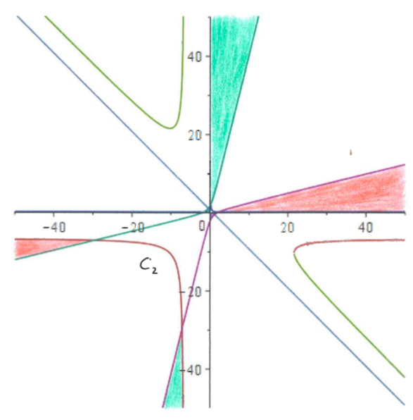

Figure 5 is just the detail near the origin of the Figure 4, and includes the cubic and its asymptotes, the quadric , but only the bounded component of the Hessian is visible (only just!), inscribed in the triangle formed by the asymptotes. In all such cases and the condition defines two open convex subcones of , but both of these satisfy the Claim made before, that part of the projectivised boundary of the subcone corresponds to an open arc of consisting of points that are visible from ; recall that in this case, the relevant branch of the Hessian is contained in the negative quadrant. This is illustrated in the two pictures, where the two open convex subcones of given by are defined by the regions shaded in red and green.
To justify that these are the correct pictures, let us consider the degenerate case where ; here the conic only intersects the projectivised boundary of at the points and . Moreover, calculation gives the formula (for this choice of ) that , which is negative on the open cone generated by and . The index at is , and so the open cone given by has two (convex) components and . From the above calculation for either , and then we have say and . If now contains a point of , then by convexity of and the fact that the points on the open cone generated by and are not in , there exists a ray of in ; this would imply the existence of another ray in , contradicting the previous deduction. We deduce that is the ray generated by and is the ray generated by . If we perturb to a point in the interior of the given region, the conic will intersect the projectivised boundary of in two points near each inflexion point, one on and one on , and defines two convex cones in ; this is the only case where intersects both the cones in defined by . This picture continues to hold true for all in the interior of the region by a continuity argument.
If is in the interior of one of the line segments of the region in question, then will define a single convex subcone of , although there will be another zero on the projectivised boundary of at an inflexion point. Since is a positive multiple of and all of is visible from , the above claim continues to hold in this case.
If is a point on the specified arc , then degenerates into two real lines intersecting at the point , each also intersecting ; so long as is a positive multiple of , then has two (convex) components , and the same argument as before proves the claim.
All the other cases are similar to the corresponding cases for , and so the claim has been verified for affine points for both the cases where the Steinian involution switches the two components of the Hessian; thus part of the boundary of consists of rays on the negative of points in an open arc in , which are not visible from .
It is a mechanical check that in both cases and , the analogous statement continues to hold if represents a point on the line at infinity . In summary therefore, assuming that is not in the closure of the half-cone on which determined by the bounded component of the Hessian, we deduce for all , that there is part of the boundary of which is not visible from but on which the Hessian vanishes. When with lying on the cone on the unbounded component of the Hessian, it follows as in Section 2 that divides into convex cones, each of which satisfies the claim.
We can therefore apply Propositions 1.1 and 1.2 to deduce that in the case where the cubic form of a Calabi–Yau threefold defines an elliptic curve with one component, with the Hessian also smooth, if there is at most one rigid non-movable surface on , then lies in a bounded family. ∎
Let us now consider the two cases where the Hessian is not smooth, namely and . We recall that in these cases we also assume that the line does not intersect the real elliptic curve at an inflexion point. Here we substitute explicit calculation for the theory of the Steinian map. As usual, if denotes a unique rigid non-movable surface on , we let denote the component of the subcone of given by containing the Kähler cone, and we set and .
Let us start with the case , where we shall assume without loss of generality that is the branch of in the positive quadrant, with asymptotes , , and is given by the two line segments : and : , , so that the cones on and meet along the rays generated by and . For an affine point , one knows when intersects (the closure of) , that is when lies on a tangent line from a point of , and one can explicitly calculate when and where is zero on . Given the class of , one is left with several cases; we leave the reader to check the case when lies on the line at infinity , and summarise below the various cases where some multiple of is of the form ; the actual calculations are tedious but easy and so will be omitted. In all these cases, we would like to argue as in the smooth case, using Proposition 1.2, to obtain a contradiction. In all cases except for (1) and (2), the quadratic will have one zero on and one on .
(1) If , , then vanishes twice on (the closure of) and is non-zero on . Moreover and so is a positive multiple of , and all of is visible from .
(2) Suppose now that , and . When , we have that and is negative on . If is a positive multiple of , we have that is empty and hence a contradiction. If is a negative multiple of , then and we deduce that there are only finitely many possible classes for as in the proof of Proposition 4.1, and hence lies in a bounded family. When , we show that vanishes once on and once on . We note that and the arc of between the two zeros of is visible from but not in the visible extremity.
(3) Suppose now that , ; then and has a zero on , , and points on are visible from but not in the visible extremity.
(4) Suppose and ; then and has a zero on , , and both and are visible from . The case when is a positive multiple of follows as in (3), by taking points on near . When is a negative multiple of , we could consider instead points on near , but these are also visible from . We find ourselves therefore left with cases where and .
(5) Suppose now , ; then and . When , we have and that has a zero on . Note that points on (near ) are visible from . When , we have and has a zero on , and points on (near ) are not visible from . If , then and defines two lines through , one of which only meets at and the other divides the interior of in two parts. The fact that points on near are visible from and points on near are not visible from covers both the cases when might be a positive or negative multiple of .
(6) Finally we suppose that and ; here we can check that and that is negative on all of , and so would again be empty.
All the other cases with then follow by symmetry. In all the cases, one can apply Proposition 1.2 to obtain the required contradiction to there being just one rigid non-movable surface, except in case (2) above and is a negative multiple of , or in case (4) above where and . In this latter case we may assume that with and is a negative multiple of . Since however , we know that there are only a finite set of possibilities for the pair of values and , using Lemma 2.2 of [6].
Proposition 4.2.
Suppose that the Picard number and the cubic in appropriate real coordinates is the Fermat cubic, and we assume that the elliptic curve does not intersect the line at an inflexion point. If contains no more than one rigid non-movable surface, then lies in a bounded family.
Proof.
As observed in the Introduction, there will be a unique rigid non-movable surface class on . From the calculations described above and the use of Proposition 2.1, we must be in one of the two exceptional cases detailed in (2) and (4) above. In the first exceptional case, we saw that there are only finitely possibilities for the class of and the argument from Proposition 4.1 shows that lies in a bounded family.
In the second exceptional case, with and is a negative multiple of . Hence as we have just argued, and can only take finitely many values, and the same is then true for . Under the assumption that the line does not contain an inflexion point of the elliptic curve, arguing as in the first part of the proof of Lemma 3.7 then shows that there are again only finitely many possibilities for . Suppose now that we are given the class , and is a negative multiple of it. Given that , an easy calculation verifies the line pair does not meet the line segment and meets the line segment in a single point, and that if then for — the quadric meets also in one point, and so the points of at which the Hessian vanishes are precisely of the form , for . A further elementary calculation verifies that for all points with for some . Hence for all the corresponding points on the boundary of , we have . We show then that the linear function is negative on all of ; if not, then for some point we have . For such a point, the index condition on implies that , and given that , this gives a contradiction when . More generally, if for a point of , then we would deduce that is numerically trivial and so . Such points will be of the form with , where we have is explicitly the linear form , whose term in has coefficient , contradicting the previous deduction.
The conclusion is that is strictly negative on all of . In particular, if we choose an integral class , then for some explicit depending on , but then for , we will have that will be negative on , in particular on any ample class , and such would not be movable. Thus we can find a bound for which is not movable for . Hence there is an upper bound on for which is movable, and so we find a finite number of classes, one of which will have a multiple which is mobile. Using the argument used previously in the proofs of Propositions 3.3 and 4.1, a finite set of integral classes may be found, at least one of which is movable and big; thus lies in a bounded family. ∎
Note that if we allow two rigid non-movable surfaces, then the cubic can be the Fermat cubic, as for instance is the case if we take a resolution of a quintic hypersurface with two simple nodes. The Fermat cubic is the only example I know where an elliptic curve occurs (defined by the ternary cubic for a Calabi–Yau threefold with ) having only one component. As we saw in Section 1, the Fermat cubic is unique in that any component of the positive index cone has boundary, part of which is curved contained in , and the rest of which has two linear parts contained in .
We now consider the remaining case, namely . As observed in the Introduction, there will be a unique rigid non-movable surface class on . We assume without loss of generality that the boundary of the relevant component of the positive index cone corresponds to the affine branch of the cubic in the quadrant , , and the appropriate line segment at infinity joining the inflexion points and . For a class , we know when and where vanishes on and we explicitly calculate when and where it vanishes on . Unsurprisingly, given that it is a limit of cases we know about with from above, is either non-zero on , or vanishes twice, except for the special case when , where . For this point, we would need to have a negative multiple of , and since only a bounded number of multiples are allowed; choosing integral we deduce as in the proofs of Propositions 3.3 and 4.1 that lies in a bounded family, given that we can bound with . Otherwise either represents a point in the affine plane other than , or represents a point at infinity. In the former case it is clear that none of is visible from , and so a contradiction may be obtained via Proposition 1.2. So we assume that is on the line at infinity (in particular ). For on the line at infinity, we know that defines a line pair intersecting at the affine point , and that the line is a further line through this point (these statements follow since they are the limit of facts we know when is near or from a direct calculation). In particular, we may identify these lines by calculating the relevant point at infinity. Clearly will not correspond to a point in the closed cone generated by and , since we know that for any ample we must have , and it is not in the open cone generated by and by Lemma 0.3. If say were a positive multiple of or , then this represents a rational point of the real elliptic curve, which lies also on the line by Lemma 0.3, contrary to the assumptions we have made, Thus without loss of generality we may assume that is a positive multiple of , with . We note in passing that if and only if . The following facts may then be checked:
(1) One of the lines of defines a plane only intersecting at the origin in and the other line (which may be explicitly calculated from ) defines a plane which cuts in two; this determines }, as the part whose boundary includes .
(2) The second line in (1) intersects the line at infinity in the point , where
Moreover the line does not intersect (and the linear form is negative on) the quadrant , if ; hence the form is negative on the non-zero elements of ; the line is the asymptote through if and the asymptote through if . For , we show that on the affine plane the form is strictly negative below the line , where . Algebraic manipulations show that in this range, and so we still have is strictly negative on the non-zero points in the closure of .
(3) If we know the class , a positive multiple of say as above, we also know and can pick any integral class in ; then for some explicit depending on . If , then for all non-zero in the closure of and all . Hence there exists such that for , we will have that is negative on all of (and in particular on the Kähler cone). Therefore there is a known upper-bound on the for which can be movable. The case when is even easier; here and we consider , with positive real roots say. Suppose now that is mobile for some ; then . Any ample class in must have , and then for all ; this implies that , which is clearly nonsense. Thus in this case too, we have found an upper-bound for the possible for which can be movable. In both cases therefore, the data produces a finite set of classes , at least one of which will have a multiple which is mobile. Using the argument used previously in the proofs of Propositions 3.3, 4.1 and 4.2, a finite set of integral classes may be found, at least one of which is movable and big; thus lies in a bounded family.
(4) We show that the class of may be assumed known up to finitely many possibilities. If , then by Propostion 2.2 of [6] there are only finitely many possible values for and . Suppose now ; if , then by Proposition 2.2 of [6] again there are still only finitely possibilities for and . We may assume therefore that , and so some positive multiple corresponds to a point at infinity with ; from this it follows that contains the open subcone of defined by . We can choose any integral in this smaller cone, and then for some explicit , we have that for some movable divisor (some multiple of which is mobile) and some integer . If , then we already have our desired big movable class, and as before we deduce boundedness and only finitely many possible values for and . We may assume therefore that , in which case the fact that yields bounds on both and . The upper-bound on will again yield only finitely many possible values for and by Proposition 2.2 of [6]. Under the assumption that the line does not meet the elliptic curve at an inflexion point, we can deduce as in the first part of the proof of Lemma 3.7 that there are only finitely many possible classes for . Having now reduced to the case when there are only finitely many possible classes for , we may run the argument from (3) to deduce the claimed result.
We have now dealt with the second case where the Hessian is singular.
Proposition 4.3.
Suppose that the Picard number and the cubic is smooth with one real component and singular Hessian, where the line does not intersect the real elliptic curve at an inflexion point. If contains no more than one rigid non-movable surface, then there will exist such a surface and lies in a bounded family.
The Main Theorem from the Introduction now follows from combining Proposition 2.4, Corollary 3.8 and Propositions 4.1 and 4.3.
References
- [1] A. Bonifant and J. Milnor, On real and complex cubic curves, Enseign. Math. 63 (2017), 21 -61.
- [2] I. Dolgachev, Classical Algebraic Geometry. CUP 2012.
- [3] D. Sullivan, Infinitesimal Computations inTopology, Publ. Math. Inst. Hautes Etud. Sci. 47 (1977) 269-331.
- [4] C.T.C. Wall, Classification problems in differential geometry V. On certain 6-manifolds, Invent. math. 1 (1966) 355-374.
- [5] P.M.H. Wilson, The Kähler Cone on Calabi–Yau threefolds, Invent. math. 107 (1992) 561-583. Erratum, Invent. math. 114 (1993) 231-233.
- [6] P.M.H. Wilson, Boundedness questions for Calabi–Yau threefolds, to appear in J. Alg. Geom. arXiv:1706.01268.