Black holes with a cosmological constant in bumblebee gravity
Abstract
In this work, we present black hole solutions with a cosmological constant in bumblebee gravity, which provides a mechanism for the Lorentz symmetry violation by assuming a nonzero vacuum expectation value for the bumblebee field. From the gravitational point of view, such solutions are spherically symmetric black holes with an effective cosmological constant and are supported by an anisotropic energy-momentum tensor, conceived of as the manifestation of the bumblebee field in the spacetime geometry. Then we calculate the shadow angular radius for the proposed black hole solution with a positive effective cosmological constant. In particular, our results are the very first relation between the bumblebee field and the shadow angular size.
Keywords:
Black Holes, Lorentz Symmetry Breaking, Black Hole Shadow, Cosmological Constantpacs
04.70.-s,04.50.Kd,11.30.Cp,04.60.-mI Introduction
The recent search for signs of the Lorentz symmetry violation at low energy regimes, due to remaining effects of quantum gravity on the Planck scale, has attracted attention in the last years Liberati2013. The Lorentz-violating effects arise in different contexts such as string theory Kostelecky1989; Kostelecky1989a; Kostelecky1989b; Kostelecky1991, noncommutative spacetime noncommutative; noncommutative2; noncommutative3, loop quantum gravity LQG; LQG2, warped brane worlds BraneLIV; BraneLIV2, and Hoava-Lifshitz gravity Horava2009, among others. A suitable framework to account for Lorentz-violating effects on the behavior of elementary particles was proposed by Colladay and Kostelecký Kostelecky1997; Kostelecky1998, based on the idea of a spontaneous Lorentz symmetry breaking in string theory Kostelecky1989, known as the Standard Model extension (SME).
The SME is an effective field theory, which includes additional gauge-invariant terms, even compatible with the observer Lorentz invariance, and is composed of contractions of the physical standard model fields with fixed background tensors Bluhm2005; Bluhm2008. Several studies involving the different sectors of the SME were carried out and allowed to raise stringent bounds on the magnitude of the Lorentz-violating parameters. Theoretical and phenomenological developments include CPT symmetry violation CPTviolation; CPTviolation2; CPTviolation3; CPTviolation4; CPTviolation5; CPTviolation6; CPTviolation7, the fermion sector fermionsector; fermionsector2; fermionsector3; fermionsector4; fermionsector5; fermionsector6; fermionsector7, the gauge CPT-odd/even sectors gaugesector; gaugesector2; gaugesector3; gaugesector4; gaugesector5; gaugesector6; gaugesector7; gaugesector8; gaugesector9, photon-fermion interactions fermioninteraction; fermioninteraction2; fermioninteraction3; fermioninteraction4; fermioninteraction5; fermioninteraction6, and radiative corrections rad1; rad1a; rad1b; rad1c; rad1d; rad1e; rad1f; rad1g; rad1h; rad1i; rad1j; rad2; rad2a; rad2b; rad2c; rad2d; rad2e.
When the gravitational interaction is taken into account, a spontaneous symmetry breaking mechanism Bluhm2005; Bluhm2008 is adopted in order to implement the local Lorentz violation and preserve the geometric constraints and conservation laws required by general relativity. An interesting and consistent approach to the spontaneous local Lorentz and diffeomorphism violations that includes the gravitational sector in the SME framework was initially discussed in Ref. Kostelecky2004. In such an approach, spacetime is assumed to be a Riemann-Cartan manifold with nonzero curvature and torsion. The presence of a self-interacting potential for the tensor fields guarantees a vacuum expectation value (VEV) whose underlying dynamics are built from vierbein and spin connections Bailey2006. Recent studies involving the SME gravitational sector include models that describe the expansion of the universe cosmology, linearized gravity linearized; linearized2, and gravitational waves GravityWaves; GravityWaves2. It is worth mentioning the existence of alternative approaches that include the violation of the Lorentz symmetry directly in the geometric structure of the theory, such as in the Randers spacetime RandersSpace; RandersSpace2; RandersSpace3 and the bipartite-Finsler spacetime Bipartite; Bipartite2.
The bumblebee models are examples of proposals that involve self-interacting tensor fields with a nonzero VEV, fields which define a privileged direction in spacetime, that is to say, they generate an anisotropic energy-momentum tensor. The simplest case is described by a vector field and was first considered in the context of string theories Kostelecky1989, with the spontaneous Lorentz-symmetry breaking triggered by a smooth quadratic potential. The bumblebee models have been studied in different contexts, whether in the curved spacetime Kostelecky2004; Bailey2006; linearized; BumblebeeCurved or in the Minkowski spacetime BumblebeeFlat; BumblebeeFlat2; BumblebeeFlat3; BumblebeeFlat4; BumblebeeFlat5; BumblebeeFlat6. As is known in the literature, some interesting effects of the bumblebee VEV arise in connection with black hole physics. In this article, we will focus on some of them.
Initial studies on black hole solutions within the Lorentz violation scenarios were carried out by Bertolami and Páramos Bertolami2005, where the authors imposed the condition of a covariant constant VEV, that is, (where is the covariant derivative), instead of the common prescription . By assuming different configurations for the background vector, those authors obtained approximated solutions in terms of the parametrized post-Newtonian parameters that are modified by the presence of the bumblebee VEV. A static and spherically symmetric black hole solution was recently built by Casana et al. Casana2018, by considering a nonminimal coupling between the Ricci tensor and the bumblebee field. The additional condition for the constant squared norm of the VEV allowed them to find an exact Schwarzschild-like solution. Modifications on the black hole thermodynamics due to the presence of the nonvanishing bumblebee VEV were pointed out in Ref. Debora2020, considering black holes geometries obtained in Refs. Bertolami2005; Casana2018. Other black hole solutions were obtained involving different bumblebee models. A Kerr-like solution was built following a similar approach Casana2020. In Ref. Euclides2020, a Reissner-Nordström solution emerged from the spontaneous Lorentz symmetric breaking triggered by a Kalb-Ramond field. Even exotic wormhole solutions have been investigated in the literature of that context Ovgun2020; Rondineli2019.
Having said all that, we follow some mentioned works and present new black holes geometries with a cosmological constant in the bumblebee model or gravity. As will see, such solutions with a cosmological constant are just possible by assuming a suitable form for the bumblebee potential. However, as we will see, the proposed geometries here are neither asymptotically anti-de Sitter nor asymptotically de Sitter. In this sense, we call them Schwarzschild-anti-de Sitter-like and Schwarzschild-de Sitter-like black holes, as much as the zero cosmological constant case, obtained by Casana et al. Casana2018, is not asymptotically flat, thus it is called Schwarzschild-like black hole. Studies on black holes with a cosmological constant are considered as very important issues since the anti-de Sitter/conformal field theory (AdS/CFT) correspondence and the observation of the accelerating expansion of the universe (in the latter case, asymptotically de Sitter or de Sitter-like black holes are justified).
From the metric obtained here, we calculated a very important observable in order to relate the bumblebee field to the spacetime geometry: the shadow angular radius. Shadow of black holes has been a seminal topic in physics recently. And the reason for that is the very first image of a black hole announced by the Event Horizon Telescope Collaboration in 2019 EHT; EHT2. Indeed, that famous image shows the shadow of M87*, the central supermassive black hole in the Messier 87 galaxy. However, the very first shadow of a black hole was calculated in the last century. In the 60s Synge Synge obtained that which we call today shadow of the Schwarzschild black hole. Then Bardeen did the same for the Kerr geometry Bardeen. In the recent years, shadows have been drawn for several black holes in many contexts Eiroa; Neves1; Neves2; Vagnozzi; Khodadi; Casana2020. According to recent works, relations between the shadow and the black hole parameters are possible in the general relativity realm or even in contexts beyond the Einsteinian context Neves1; Neves2; Vagnozzi; Kumar; Khodadi. Our focus here is in a model beyond general relativity.
This article is structured as follows: In Section II the framework is presented, and both the Schwarzschild-anti-de Sitter-like and the Schwarzschild-de Sitter-like black holes are built in the bumblebee gravity, some features are discussed like horizons, singularity, and the energy-momentum tensor for those black holes. Section III speaks of the shadow angular radius of the Schwarzschild-de Sitter-like geometry, and the influence of the Lorentz-violating parameter on this phenomenon is pointed out. The final comments are in Section IV. We adopt geometrized units in our calculations, i.e., , where is the Newtonian constant, and is speed of light in vacuum.
II Constructing black holes in the bumblebee gravity
II.1 The adopted framework
As we pointed out, bumblebee models provide a simple mechanism for studying the spontaneous breaking of the Lorentz symmetry in the gravitational scenario. These types of models have a nontrivial VEV that affects the dynamics of other fields coupled to the bumblebee field, preserving geometric structures and conservation laws compatible with a usual pseudo-Riemannian manifold from general relativity Kostelecky2004; Bluhm2005.
Among several possibilities of models that are able to break the Lorentz symmetry, there is the simplest action form involving a vector field , the bumblebee field, in a torsion-free spacetime written as
| (1) | |||||
where is the gravitational coupling constant, is the cosmological constant, and plays the role of a coupling constant that accounts for the nonminimum interaction between the bumblebee field and the Ricci tensor or geometry (with mass dimension ) Bailey2006; linearized. Also, one has or the bumblebee field strength, and describes the matter and additional couplings with the field . The potential is responsible for triggering the spontaneous Lorentz violation in case of the bumblebee field assumes a nonzero VEV , satisfying the condition . It is worth emphasizing that the quantity is a positive real number, and the sign implies that is timelike or spacelike, respectively. The model described by the action (1) and other versions involving different couplings or choices of the potential have been investigated in a variety of contexts (as mentioned in Introduction).
The gravitational field equations in the bumblebee context or gravity can be directly obtained by varying the action (1) with respect to the metric tensor , while keeping the bumblebee field fixed. That procedure yields
| (2) |
as modified gravitational field equations, in which is the Einstein tensor and the operator ′ means derivative with respect to the potential argument. In the general case, and are the energy-momentum tensors of the bumblebee field and of the matter field, respectively. In order to solve Eq. (2), it is necessary to choose a bumblebee potential and a metric Ansatz with some symmetry, like the spherical or the axial symmetry. By doing that, one obtains a set of equations and, solving them, a full metric. Here we focus on the spherical symmetry and comment some potentials as options to get a full black hole metric, whether with or without a cosmological constant.
The action (1) also provides an equation of motion for . By varying that action in this time with respect to the bumblebee field leads to
| (3) |
With all framework introduced, in which we do not consider a coupling between the bumblebee field and the matter field, we will apply it to the nonzero cosmological constant case, generating then black holes with a cosmological constant. But before that, we comment a previous result that involves a null cosmological constant.
II.2 The case
In this framework, an exact black hole solution without a cosmological constant was constructed by Casana et al. Casana2018, also known as the Schwarzschild-like black hole. According to the authors, a spherically symmetric spacetime in the absence of both matter and a cosmological constant () was interpreted as a Schwarzschild-like black in the bumblebee gravity, from a radial bumblebee field written as
| (4) |
In the coordinates , the general spherical Ansatz used by the authors (and adopted here) is given by
| (5) |
Adopting both the mentioned Ansatz and the condition , one has the radial component of the bumblebee field when it assumes the VEV, i.e.,
| (6) |
As we can see, contrary to Bertolami and Páramos Bertolami2005, the authors of Ref. Casana2018, from Eq. (6), have , which is the same form of the bumblebee field that we will adopt next. It is worth pointing out that the vanishing condition for the covariant derivative is just possible for special spacetimes with a geometrical constraint that comes from the underlying pseudo-Riemann geometry assumption.
With that Ansatz plus the mentioned bumblebee form and assuming , the following metric
| (7) | |||||
is a solution of the modified field equations (2). The metric (7) is also called Schwarzschild-like geometry. The bumblebee field or the Lorentz-violating parameter is represented in that metric by , and the parameter stands for the usual mass of the Schwarzschild black hole in the limit . Note that the condition (4) and the potential choice imply that the field stays frozen in its VEV , that is to say, (vacuum condition) and the assumption ensures that the field is in the minimum of the potential. Besides that, since the background field is a spacelike vector purely radial, its associated field strength is identically null, i.e., .
A solution like (7) resembles that one obtained by Seifert in Ref. Seifert, in which a Lorentz-violating topological defect was studied. In the mentioned paper, the author presented a topological defect solution from a Lorentz symmetry breaking triggered spontaneously by a tensor field, namely, a rank-two antisymmetric tensor field. Such a solution was interpreted as a vacuum monopole solution. As we said, such a monopole solution reseambles (7), but it does not approach asymptotically the line element (7) due to a different -dependence. On the other hand, according to Ref. Seifert2, for the Lorentz symmetry breaking triggered by a vector field, which is just the case considered here, a domain wall (another kind of topological defect) solution was obtained only when a timelike vector was adopted. In this sense, the possibility of a topological defect solution for a spacelike vector (like the bumblebee field adopted here) is prohibited.
From the metric (7), it is clear to see that the event horizon does not depend on . As is well known, considering a metric like (5), zeros of provide the localization of horizons. As we can directly read, for the metric (7) one has , the same value of the event horizon of the Schwarzschild black hole. In the same way, as we will see, the photon sphere is located at , like Schwarzschild’s. Such a surface is responsible for the black hole shadow. On the other hand, as pointed out by Casana et al. Casana2018, the light bending and the perihelion advance bring out the Lorentz-violating parameter and its (possible) tiny influence.11 1 In Ref. Casana2018, there are upper bounds on the parameter from, for example, light deflection, time delay of light, and perihelion advance of the planet Mercury. The most stringent upper bound on the Lorentz-violating parameter is to date. It is worth emphasizing that the solution (7) cannot be converted into the standard Schwarzschild solution for a nonzero value of by means a suitable coordinate transformation Casana2018; Debora2020. In this sense, the metric (7) is an entirely new spacetime metric.
II.3 The case
Following the approach outlined above, we will now investigate some effects of the Lorentz violation in the presence of a nonzero cosmological constant on the model described by the action (1). More specifically, we are interested in obtaining an exact black hole solution in the presence of a cosmological constant, a geometry similar to either the Schwarzschild-anti-de Sitter black hole or the Schwarzschild-de Sitter black hole (depending on the sign of the cosmological constant). One route to be explored here is to relax the vacuum conditions, i.e., and assumed by Casana et al. Casana2018. A simple example of a potential that satisfies such conditions is clearly provided by a smooth quadratic form
| (8) |
where is a constant, and is a generic potential argument. In this case, the VEV is solution of . Another simple choice of potential consists of a linear function
| (9) |
where now is a Lagrange-multiplier field Bluhm2008. Note that the equation of motion for the Lagrange-multiplier ensures the vacuum condition , and then for any field on-shell. However, for the linear functional form (9), it follows that when the field is nonzero, so additional contributions from the potential can modify the Einstein equations. Since has no kinetic terms, it is auxiliary and cannot propagate. However, it is also an additional degree of freedom that appears in the equations of motion. In fact, the equations of motion for the metric (2) and the bumblebee field (3) provide constraints on the field . Moreover, in order to be well defined, all bumblebee models require explicit initial conditions on the field excitations about vacuum values. Like the bumblebee field, the Lagrange multiplier can also be expanded around its vacuum value as
| (10) |
For our purpose here, it is convenient to fix the initial conditions taking , which implies that the field remains frozen in its VEV. This is a similar hypothesis used for the bumblebee field in Ref. Casana2018. A priori, could depend on the spacetime position, but it is sufficient to assume it as a real constant. Thus, in what follows, the on-shell value of is given by , with its value fixed from the equations of motion (2) or (3) in terms of other parameters of the model.
It is worth noting that the action (1) with the conditions , adopted by Casana et al. Casana2018, will provide a black hole solution from the Ansatz (5) only if . A black hole solution with a nonzero cosmological constant needs a different potential, in the case of a solution with the relation exhibited in the Schwarzschild-like black hole (7). Therefore, in order to build black holes with a cosmological constant, we assume, for that purpose, the linear potential written as
| (11) |
where is assumed radial-like (4). With such a potential and the Ansatz (5), one has three independent equations from Eq. (2) because . That is to say, our system of equations reads
| (12) |
| (13) | |||
| (14) |
As we can see, our system shows three independent equations and two unknown functions ( and ). A third would come from the matter energy-momentum tensor with a suitable equation of state. In our case, without a matter field, that function is zero.
Equation (12) is a differential equation which involves just . Thus, its solution is directly given by
| (15) |
where is an integration constant interpreted as some sort of mass parameter of the Schwarzschild geometry. By making , we hope to recover the Schwarzschild-like solution. In this sense, for that purpose.
In order to generate a solution of Eqs. (12)-(14) similar to the case, we use the mentioned relation between the metric terms, . Thus from Eq. (15), one has
| (16) |
as solution of our system. Such a relation between the metric terms provides and an appropriate solution for the system of equations (12)-(14) even with a nonzero cosmological constant. However, with the potential given by (11), a solution of this type will be possible if and only if
| (17) |
The constraint (17) is a conditio sine qua non in order to generate a metric with a cosmological constant from the modified Einstein equations (2) and the potential (11). This is the constraint on the field coming from the modified Einstein field equations as mentioned earlier.
With all metric terms known, namely (15) and (16), our proposed metric with spherical symmetry and a cosmological constant reads
| (18) |
in which, by convenience, we conceive of as an effective cosmological constant. It is worth mentioning that the constraint (17) also guarantees the energy conservation of the bumblebee energy-momentum tensor. Indeed,
| (19) |
for all components, except for the component that asks that constraint in order to satisfy the energy-momentum conservation. And the equation of motion for the bumblebee field (3) is also verified by using the constrain (17) for the nonzero cosmological constant case.
The metric (18) is richer than the metric (7) that excludes a cosmological constant. As will see, the bumblebee field influence is found even on the horizons, contrary to the Schwarzschild-like solution in which the event horizon radius is the same of the Schwarzschild black hole. In particular, the last part of this article will show the influence of the bumblebee field on the shadow angular radius. Those influences are a consequence of the Lorentz symmetry violation, which is translated into geometry or into the general relativity language from a privileged spacetime direction or an anisotropic fluid. This is noteworthy from the total energy-momentum tensor of the metric (18) given by
| (20) |
in which
| (21) |
with and playing the role of the energy density and the radial pressure, respectively, and is the tangential pressure. Then the anisotropic feature of the spacetime (18) gets evident, the radial and tangential pressures are different. As we can see, in particular, the radial pressure is always negative when , which is the Schwarzschild-de Sitter-like case as we will indicate later. A relation between the bumblebee field (specifically its potential) and a de Sitter phase in cosmology was already indicated in Ref. cosmology and it appears in the gravitational context once again here.
It is worth emphasizing that the metric (18) is neither asymptotically de Sitter nor asymptotically anti-de Sitter. That is, we cannot write that metric in a particular form such that, in the end of the day,
| (22) |
The factor before , namely , forbids the above limit. According to Ref. Debora2020 mentioned before, that factor also forbids a coordinate transformation that turns the Schwarzschild-like black hole into the Schwarzschild black hole. The same argument can be adopted here, for our metric uses the relation such as the Schwarzschild-like black hole. Therefore, the metric (18) is not converted into either the Schwarzschild-anti-de Sitter black hole or the Schwarzschild-de Sitter black hole.
Another feature of the metric (18) regards to real or “fictitious” singular points. The former is the physical singularity that appears by taking, for example, the limit of the Kretschmann scalar (built from the Riemann tensor), which is given by
| (23) | |||||
The Schwarzschild-like singularity is present only at (considering ). The mentioned “fictitious” singular points are, indeed, a bad choice of the coordinate system. As we said, zeros of give us not a “physical singularity”, but special surfaces, horizons, which depend on the sign of in the metric (18).
The metric (18) is also independent of two coordinates: and . Thus, that geometry possesses two Killing vector fields ( and ) related to two conserved quantities, energy and angular momentum (both will be useful later for the geodesic motion).
Schwarzschild-anti-de Sitter-like black hole
Assuming , we have a Schwarzschild-anti-de Sitter-like solution. And its spacetime structure is given by a unique horizon, the event horizon, whose radius is
| (24) |
with
| (25) |
The relation between the parameters of the black hole (18) and the event horizon radius is indicated in Fig. 1. As we can see, for large values of , the symmetry breaking parameter, , decreases the horizon radius.
In this case, , the unique Killing surface coincides with the event horizon. The Killing surfaces localization is calculated from , they are surfaces where the Killing vector field is null or lightlike. Above all, from that surface to infinity, the Killing vector field is timelike in the Schwarzschild-anti-de Sitter-like case. In this entire region, , static observers are viable ones.

Schwarzschild-de Sitter-like black hole
On the other hand, the Schwarzschild-de Sitter-like black hole appears from . In this case, the spacetime structure presents two horizons: the event horizon, , and the cosmological horizon, . However, in order to provide two horizons (two real roots of ), the metric parameters or the effective cosmological constant should obey the following inequality:
| (26) |
With one has the well-known Schwarzschild-de Sitter condition to generate two horizons.22 2 For a review on the Schwarzschild-anti-de Sitter and Schw- arzschild-de Sitter geometries, see Ref. Stuchlik. And for , our metric shows an extreme case, in which . Analytic expressions for the event and the cosmological horizons are, respectively,
| (27) |
| (28) |
with . As we can see in Fig. 2, the Lorentz-violation parameter, , modifies the spacetime structure, it decreases the cosmological horizon radius and, at the same time, increases the event horizon radius for considerable values of . The region is the so-called domain of outer communication. In that region, observers may communicate with each other, thus there is no horizon in that region. But an observer beyond the cosmological horizon may be invisible according to someone inside the domain of outer communication. In the domain of outer communication, observers can be static ones, and the Killing vector field is timelike in that region (consequently, having both the spherical symmetry and the mentioned timelike Killing vector makes Eq. (18) a static spacetime). In the next section, we calculate the shadow angular radius of the metric (18) as seen by a static observer in the domain of outer communication.


III The shadow angular radius
The black hole shadow is a dark region in the bright sky caused by a black hole and its huge gravitational field or the intense light deflection. Here we are interested in calculating the angular radius of the shadow generated by the black hole (18) for , the Schwarzschild-de Sitter-like case (more appropriate from the cosmological point of view). As we mentioned, our observer will be at rest in the domain of outer communication, that is to say, our observer is a static one. The shadow silhouette is given by unstable orbits (circular unstable orbits for our metric) outside the event horizon. In such orbits, photons may either go into the black hole or go to the opposite direction, reaching, for example, our observer. Therefore, we need the null geodesic equations in order to obtain such special orbits and trace them to the observer position.
Geodesics are calculated from the Lagrangian
| (29) |
where dot means derivative with respect to the affine parameter of the curve (indicate here by ). In particular, an equatorial null geodesic () for the metric (18) becomes simply
| (30) |
As we said, our proposed metric has and as two Killing vector fields that, consequently, yield two conserved quantities. The first one () provides the energy conservation, and the second one () gives us the angular momentum conservation. Therefore, photons along the geodesics (30) have both conserved energy and angular momentum given by
| (31) |
As is known from textbooks, the geodesic equations from a spacetime with spherical symmetry like (18) may be written as a conservation equation for each photon, a familiar equation like
| (32) |
in which the gravitational potential and the energy are defined as
| (33) |
| (34) |
The condition of unstable orbits ( and ) that compose the black hole shadow give us the following radius: . This is the photon sphere radius, and such a sphere is the surface that creates the shadow silhouette. Therefore, in order to measure the shadow angular radius, our observer will be beyond the photon sphere. As we can see, that radius is the same of the Schwarzschild photon sphere, as much as of the Schwarzschild-de Sitter sphere. The Lorentz-violating parameter does not modify such a result (see Fig. 3).
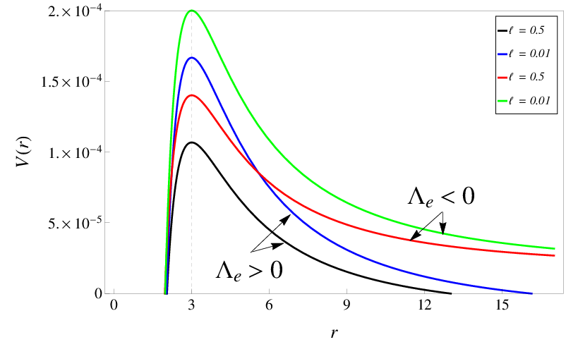
Circular orbits implies , thus Eq. (30) delivers a useful ratio
| (35) |
With the aid of the photon sphere radius, , photons that compose the shadow silhouette present the following constant energy-angular momentum ratio:
| (36) |

We are going to follow the approach presented in Ref. Perlick where the shadow angular radius was calculated for the Schwarzschild-de Sitter black hole. In that approach, our static observer—as we said—is in the domain of outer communication, between the photon sphere and the cosmological horizon. His/her radial coordinate is . According to Fig 4, the shadow angular radius is defined as
| (37) |
In order to obtain the angle , we adopt the isotropic coordinate system, in which angles are invariant in comparison with the Euclidian space. With that coordinate system, our two-dimensional metric (spatial components with ) becomes conformal to the two-dimensional Euclidian space in spherical coordinates and can be written as
| (38) |
from the following transformations
| (39) |
| (40) |
in which is the conformal factor. Therefore, from the above relations, it is easy to get
| (41) | |||||
The term comes directly from the geodesic equation (30), and with a useful trigonometric relation, namely , the following angle is obtained
| (42) |
For a static observer at in the domain of outer communication, the shadow angular radius is obtained from orbits with the calculated energy-angular momentum ratio (36), that is to say, orbits from the photon sphere. Then substituting Eq. (36) into Eq. (42), we have the sought-after relation
| (43) |
As we can see, the above relation equals the result obtained in Ref. Perlick by imposing , which is the Schwarzschild-de Sitter black hole studied in the mentioned article. Moreover, with , we recover the shadow angular radius of the Schwarzschild geometry. As we mentioned earlier, a geometry like (18), with , cannot be converted into either the usual Schwarzschild solution (), or the Schwarzschild-anti-de Sitter solution (), or the Schwarzschild-de Sitter solution () from a suitable coordinate transformation. Therefore, the parameter cannot be absorbed into the cosmological constant, and then the result (43) does not turn into the shadow angular radius of the Schwarzschild-de Sitter black hole as calculated in Ref. Perlick.

Some highlights of the result (43): for , the shadow angular radius is zero, i.e., the sky is entirely bright for our observer. On the other hand, for , the shadow angular radius is maximum, thus observer’s sky is half bright and half dark. Lastly, according to Fig. 5, we can see the influence of the Lorentz-violating parameter on the shadow. The influence of the parameter on the shadow was commented in Ref. Casana2020 where a Kerr-like black hole was built in the bumblebee gravity. That parameter increases the shadow deformation when a rotating black hole is considered. But, for the first time in the literature, the influence of the Lorentz-violating parameter on the shadow angular radius was straightforwardly indicated. Such a parameter—that makes the action (1) non-Lorentz invariant and generates anisotropic spacetimes with a privileged direction—decreases the shadow angular radius, as we just read in Fig 5.
IV Final remarks
The bumblebee gravity is a Lorentz-violating model in which the VEV of the bumblebee field is nonzero and provides, for example, a privileged spacetime direction by means of the Lorentz-violating parameter included in the spacetime metric. Here we built black holes solutions with an effective cosmological constant, which comes from a suitable choice for the bumblebee potential. Such an effective cosmological constant could be either positive or negative. In the first case, we have a Schwarzschild-de Sitter-like black hole. And for the second case, a Schwarzschild-anti-de Sitter-like black hole. The spacetime structure of both black holes was studied, and the influence of the Lorentz-violating parameter was pointed out, i.e., that parameter may increase or decrease the horizons radii depending on the sign of the effective cosmological constant.
The second part of this article was dedicated to the study of the shadow angular radius in the case of a positive and effective cosmological constant, which is the most appropriate case for a cosmological context. As we said, the Lorentz-violating parameter influence on the shadow angular radius—as far as we know, obtained for the first time in the literature here—decreases the shadow angular size.
Acknowledgments
We thank Celio Muniz for comments during the article development and an anonymous referee for valuable points raised in the the review process. RVM thanks Fundação Cearense de Apoio ao Desenvolvimento Científico e Tecnológico (FUNCAP), Coordenação de Aperfeiçoamento de Pessoal de Nível Superior (CAPES), and Conselho Nacional de Desenvolvimento Científico e Tecnológico (CNPq, Grant no 307556/2018-2) for the financial support. JCSN also thanks Coordenação de Aperfeiçoamento de Pessoal de Nível Superior (CAPES, Finance Code 001) for the financial support.
References
- (1) S. Liberati, Class. Quantum Gravity 30, 133001 (2013).
- (2) V. A. Kostelecký and S. Samuel, Phys. Rev. D 39, 683 (1989).
- (3) V. A. Kostelecký and S. Samuel, Phys. Rev. Lett. 63, 224 (1989).
- (4) V. A. Kostelecký and S. Samuel, Phys. Rev. D 40, 1886 (1989).
- (5) V. A. Kostelecký and R. Potting, Nucl. Phys. B 359, 545 (1991).
- (6) S. M. Carroll, J. A. Harvey, V. A. Kostelecky, C. D. Lane, and T. Okamoto, Phys. Rev. Lett. 87, 141601 (2001).
- (7) I. Mocioiu, M. Pospelov, and R. Roiban, Phys. Lett. B 489, 390 (2000).
- (8) A. F. Ferrari, M. Gomes, J. R. Nascimento, E. Passos, A. Yu. Petrov, and A. J. da Silva, Phys. Lett. B 652, 174 (2007).
- (9) R. Gambini and J. Pullin, Phys. Rev. D 59, 124021 (1999).
- (10) J. R. Ellis, N. E. Mavromatos, and D. V. Nanopoulos, Gen. Relativ. Gravit. 32, 127 (2000).
- (11) T. G. Rizzo, J. High Energy Phys. 1011, 156 (2010).
- (12) V. Santos and C. A. S. Almeida, Phys. Lett. B 718, 1114 (2013).
- (13) P. Hoava, Phys. Rev. D 79, 084008 (2009).
- (14) D. Colladay and V. A. Kostelecký, Phys. Rev. D 55, 6760 (1997).
- (15) D. Colladay and V. A. Kostelecký, Phys. Rev. D 58, 116002 (1998).
- (16) R. Bluhm, V.A. Kostelecký, Phys. Rev. D 71, 065008 (2005).
- (17) R. Bluhm, S.-H. Fung, V.A. Kostelecký, Phys. Rev. D 77, 065020 (2008).
- (18) R. Bluhm, V. A. Kostelecký, and N. Russell, Phys. Rev. Lett. 79, 1432 (1997).
- (19) R. Bluhm, V. A. Kostelecký, and N. Russell, Phys. Rev. D 57, 3932 (1998).
- (20) R. Bluhm, V. A. Kostelecký, and N. Russell, Phys. Rev. Lett. 82, 2254 (1999).
- (21) V. A. Kostelecký and C. D. Lane, Phys. Rev. D 60, 116010 (1999).
- (22) R. Bluhm and V. A. Kostelecký, Phys. Rev. Lett. 84, 1381 (2000).
- (23) R. Bluhm, V. A. Kostelecký, and C. D. Lane, Phys. Rev. Lett. 84, 1098 (2000).
- (24) R. Bluhm, V. A. Kostelecký, C. D. Lane, and N. Russell, Phys. Rev. Lett. 88, 090801 (2002).
- (25) V. A. Kostelecký and C. D. Lane, J. Math. Phys. 40, 6245 (1999).
- (26) V. A. Kostelecký and R. Lehnert, Phys. Rev. D 63, 065008 (2001).
- (27) D. Colladay and V. A. Kostelecký, Phys. Lett. B 511, 209 (2001).
- (28) R. Lehnert, Phys. Rev. D 68, 085003 (2003).
- (29) R. Lehnert, J. Math. Phys. 45, 3399 (2004).
- (30) B. Altschul, Phys. Rev. D 70, 056005 (2004).
- (31) G. M. Shore, Nucl. Phys. B 717, 86 (2005).
- (32) S. M. Carroll, G. B. Field, and R. Jackiw, Phys. Rev. D 41, 1231 (1990).
- (33) A. A. Andrianov and R. Soldati, Phys. Rev. D 51, 5961 (1995).
- (34) A. A. Andrianov and R. Soldati, Phys. Lett. B 435, 449 (1998).
- (35) A. A. Andrianov, R. Soldati, and L. Sorbo, Phys. Rev. D 59, 025002 (1998).
- (36) A. P. Baêta Scarpelli, H. Belich, J. L. Boldo, and J. A. Helayël-Neto, Phys. Rev. D 67, 085021 (2003).
- (37) R. Lehnert and R. Potting, Phys. Rev. Lett. 93, 110402 (2004).
- (38) C. Kaufhold and F. R. Klinkhamer, Nucl. Phys. B 734, 1 (2006).
- (39) B. Altschul, Phys. Rev. D 75, 105003 (2007).
- (40) H. Belich, L. D. Bernald, P. Gaete, and J. A. Helayël-Neto, Eur. Phys. J. C 73, 2632 (2013).
- (41) M. Schreck, Phys. Rev. D 86, 065038 (2012).
- (42) G. Gazzola, H. G. Fargnoli, A. P. Baêta Scarpelli, M. Sampaio, and M. C. Nemes, J. Phys. G 39, 035002 (2012).
- (43) A. P. Baêta Scarpelli, J. Phys. G 39, 125001 (2012).
- (44) B. Agostini, F. A. Barone, F. E. Barone, P. Gaete, and J. A. Helayël-Neto, Phys. Lett. B 708, 212 (2012).
- (45) L. C. T. Brito, H. G. Fargnoli, and A. P. Baêta Scarpelli, Phys. Rev. D 87, 125023 (2013).
- (46) S. Tizchang, R. Mohammadi, and S. Xue, Eur. Phys. J. C 79, 224 (2019).
- (47) R. Jackiw and V.A. Kosteleck´y, Phys. Rev. Lett. 82, 3572 (1999).
- (48) J.-M. Chung, Phys. Rev. D 60, 127901 (1999).
- (49) M. Perez-Victoria, Phys. Rev. Lett. 83, 2518 (1999).
- (50) J.-M. Chung and B.K. Chung, Phys. Rev. D 63, 105015 (2001).
- (51) G. Bonneau, Nucl. Phys. B 593, 398 (2001).
- (52) M. Perez-Victoria, J. High Energy Phys. 0104, 032 (2001).
- (53) O.A. Battistel and G. Dallabona, J. Phys. G 27, L53 (2001).
- (54) O.A. Battistel and G. Dallabona, Nucl. Phys. B 610, 316 (2001).
- (55) A. P. B. Scarpelli, M. Sampaio, M.C. Nemes, and B. Hiller, Phys. Rev. D 64, 046013 (2001).
- (56) O.A. Battistel and G. Dallabona, J. Phys. G 28, L23 (2002).
- (57) B. Altschul, Phys. Rev. D 70, 101701(R) (2004).
- (58) T. Mariz, J.R. Nascimento, E. Passos, R.F. Ribeiro, and F.A. Brito, J. High Energy Phys. 0510, 019 (2005).
- (59) J.R. Nascimento, E. Passos, A.Yu. Petrov, and F.A. Brito, J. High Energy Phys. 0706, 016 (2007).
- (60) A.P.B. Scarpelli, M. Sampaio, M.C. Nemes, and B. Hiller, Eur. Phys. J. C 56, 571 (2008).
- (61) F.A. Brito, J.R. Nascimento, E. Passos, and A.Yu. Petrov, Phys. Lett. B 664, 112 (2008).
- (62) F.A. Brito, L.S. Grigorio, M.S. Guimaraes, E. Passos, and C. Wotzasek, Phys. Rev. D 78, 125023 (2008).
- (63) O.M. Del Cima, J.M. Fonseca, D.H.T. Franco, and O. Piguet, Phys. Lett. B 688, 258 (2010).
- (64) V.A. Kostelecký, Phys. Rev. D 69, 105009 (2004).
- (65) Q. G. Bailey and V. A. Kostelecký, Phys. Rev. D 74, 045001 (2006).
- (66) D. Capelo, J. Páramos, Phys. Rev. D 91 (10), 104007 (2015).
- (67) R. V. Maluf, V. Santos, W. T. Cruz, and C. A. S. Almeida, Phys. Rev. D 88, 025005 (2013).
- (68) R. V. Maluf, C. A. S. Almeida, R. Casana, and M. M. Ferreira, Jr., Phys. Rev. D 90, 025007 (2014).
- (69) V. A. Kostelecký, A. C. Melissinos, and M. Mewes, Phys. Lett. B 761, 1 (2016).
- (70) V. A. Kostelecký and M. Mewes, Phys. Lett. B 757, 510 (2016).
- (71) V.A. Kostelecký, N. Russell, R. Tso, Phys. Lett. B 716, 470 (2012).
- (72) J. E. G. Silva, C.A.S. Almeida, Phys. Lett. B 731, 74 (2014).
- (73) J.E.G. Silva, R.V. Maluf, C.A.S. Almeida, Phys. Lett. B 766, 263 (2017).
- (74) V. A. Kostelecký, N. Russell, R. Tso, Phys. Lett. B 716, 470 (2012).
- (75) J. E. G. Silva, R. V. Maluf, C. A. S. Almeida, Phys. Lett. B 798, 135009 (2019).
- (76) Zonghai Li and Ali Övgün, Phys. Rev. D 101, 024040 (2020).
- (77) Sean M. Carroll, Timothy R. Dulaney, Moira I. Gresham, Heywood Tamx, Phys. Rev. D 79, 065011 (2009).
- (78) R. Bluhm, N.L. Gagne, R. Potting, A. Vrublevskis, Phys. Rev. D 77, 125007 (2008).
- (79) R. Bluhm, N.L. Gagne, R. Potting, A. Vrublevskis, Phys. Rev. D 79, 029902 (2009) (Erratum).
- (80) C.A. Hernaski, Phys. Rev. D 90, 124036 (2014).
- (81) R. V. Maluf, J. E. G. Silva, C. A. S. Almeida, Phys. Lett. B 749, 304 (2015)
- (82) C. A. Escobar and A. Martín-Ruiz, Phys. Rev. D 95, 095006 (2017).
- (83) O. Bertolami, J. Páramos, Phys. Rev. D 72, 044001 (2005).
- (84) R. Casana, A. Cavalcante, F. P. Poulis, E. B. Santos, Phys. Rev. D 97, 104001 (2018).
- (85) D. A. Gomes, R. V. Maluf, C. A. S. Almeida, Annals of Physics 418, 168198 (2020).
- (86) C. Ding, C. Liu, R. Casana, A. Cavalcante, Eur. Phys. J. C 80, 178 (2020).
- (87) L. A. Lessa, J. E. G Silva, R. V. Maluf, C. A. S. Almeida, Eur. Phys. J. C, 80, 335 (2020).
- (88) A. Övgün, K. Jusufi, and I. Sakalli, Phys. Rev. D 99, 024042 (2019).
- (89) R. Oliveira, D. M. Dantas, V. Santos, C. A. S. Almeida, Class. Quantum Gravity 36 (10), 105013 (2019).
- (90) K. Akiyama et al. (The Event Horizon Telescope Collaboration), Astrophys. J. Lett. 875, L1 (2019).
- (91) K. Akiyama et al. (The Event Horizon Telescope Collaboration), Astrophys. J. Lett. 875, L6 (2019).
- (92) J. L. Synge, Mon. Not. R. Astron. Soc. 131, 463 (1966).
- (93) J. M. Bardeen, Timelike and null geodesics in the Kerr metric, in Black Holes, edited by C. DeWitt and B. DeWitt (Gordon and Breach, New York, 1973), p. 215.
- (94) E. F. Eiroa and C. M. Sendra, Eur. Phys. J. C 78, 91 (2018).
- (95) J. C. S. Neves, Eur. Phys. J. C 80, 343 (2020).
- (96) J. C. S. Neves, Eur. Phys. J. C 80, 717 (2020).
- (97) S. Vagnozzi, and L. Visinelli, Phys. Rev. D 100, 024020 (2019).
- (98) A. Allahyari, M. Khodadi, S. Vagnozzi, and D. F. Mota, J. Cosmol. Astropart. Phys. 02, 003 (2020).
- (99) R. Kumar, A. Kumar, and S. G. Ghosh, Astrophys. J. 896, 89 (2020).
- (100) M. D. Seifert, Phys. Rev. Lett. 105, 201601 (2010).
- (101) M. D. Seifert, Phys. Rev. D 82, 125015 (2010).
- (102) Z. Stuchlik, and S. Hledik, Phys. Rev. D 60 044006 (1999).
- (103) V. Perlick, O. Yu. Tsupko, and G. S. Bisnovatyi-Kogan, Phys. Rev. D 97 104062 (2018)