1000
Deep Learning-based Resource Allocation
For Device-to-Device Communication
Abstract
In this paper, a deep learning (DL) framework for the optimization of the resource allocation in multi-channel cellular systems with device-to-device (D2D) communication is proposed. Thereby, the channel assignment and discrete transmit power levels of the D2D users, which are both integer variables, are optimized to maximize the overall spectral efficiency whilst maintaining the quality-of-service (QoS) of the cellular users. Depending on the availability of channel state information (CSI), two different configurations are considered, namely 1) centralized operation with full CSI and 2) distributed operation with partial CSI, where in the latter case, the CSI is encoded according to the capacity of the feedback channel. Instead of solving the resulting resource allocation problem for each channel realization, a DL framework is proposed, where the optimal resource allocation strategy for arbitrary channel conditions is approximated by deep neural network (DNN) models. Furthermore, we propose a new training strategy that combines supervised and unsupervised learning methods and a local CSI sharing strategy to achieve near-optimal performance while enforcing the QoS constraints of the cellular users and efficiently handling the integer optimization variables based on a few ground-truth labels. Our simulation results confirm that near-optimal performance can be attained with low computation time, which underlines the real-time capability of the proposed scheme. Moreover, our results show that not only the resource allocation strategy but also the CSI encoding strategy can be efficiently determined using a DNN. Furthermore, we show that the proposed DL framework can be easily extended to communications systems with different design objectives.
Index Terms:
Multi-channel wireless communications systems, interference channel, D2D transmission, deep learning, distributed operation, resource allocation, CSI sharing.I Introduction
In wireless communication systems (WCS), efficient resource allocation is important to achieve high system performance. Resource allocation for WCS has been studied for several decades for different types of systems including cognitive radio (CR) [1, 2, 3], device-to-device (D2D) [4, 5, 6, 7], vehicle-to-everything (V2X) [8, 9], and non-orthogonal multiple access (NOMA) [10, 11] communication systems.
Existing resource allocation schemes typically aim to maximize spectral efficiency (SE) [3, 8, 10] or energy efficiency (EE) [5, 6] or to minimize the total transmit power [1, 11] under different constraints, e.g., quality-of-service (QoS) [11, 7] and interference [6, 1, 2] constraints. The resource allocation in WCS becomes very challenging when multiple users transmit data simultaneously over the same radio resource, e.g., in D2D WCS, because of the resulting multi-user interference. In this case, resource allocation algorithm design leads to a nonconvex optimization problem which is generally difficult to solve in an efficient manner due to its NP-hardness.
In the literature, most existing resource allocation schemes [12, 6, 7] involve iterative algorithms which limits their applicability in practice where real-time operation is essential [13, 14]. In particular, iterative methods may take a long time to converge when the number of users or resource allocation variables is large. Moreover, such analytical solutions for resource allocation are taylor-made for a specific problem and a completely new solution has to be developed if the problem formulation changes only slightly, e.g., a different objective function or additional constraints are considered, which further limits the applicability of this approach. Deep learning (DL)-based schemes can overcome the aforementioned shortcomings of current resource allocation designs.
I-A Application of DL in WCS
DL, which is based on deep neural networks (DNNs), has recently seen a surge in interest in different application domains, mainly due to its remarkable advantages over conventional methods. For example, image classification based on DL has even surpassed human-level performance [15]. In DL, a DNN model is trained to minimize the adopted loss function based on a large amount of data and the back propagation algorithm without relying on an explicit hand-crafted mathematical formulation of the system model. Although DL has been extensively studied in the fields of computer vision and natural language processing, only recently, it has been seriously considered for the design of WCS [16] regarding problems such as channel estimation, data detection, and classification of wireless signals.
Channel estimation and data detection based on DL were studied for orthogonal frequency-division multiplexing (OFDM) [17], filter bank multicarrier modulation [18], multiple-input and multiple-output (MIMO) [19], millimeter-wave (mmWave) MIMO [20], and molecular communication [21] systems. Moreover, the authors of [22] studied DL-based channel estimation and detection for MIMO systems with 1-bit analog-to-digital converters. Furthermore, in [23], a DL-based channel state information (CSI) feedback scheme for massive MIMO systems was proposed.
Regarding the classification of wireless signals, it was shown in [24] and [25] that the modulation format and the type of data traffic can be determined accurately with DNNs. DL was also applied for cooperative spectrum sensing in CR systems [26], where a DNN-based cooperative spectrum sensing strategy was proposed. Moreover, DL was exploited for the design of encoders and decoders using a DNN-based autoencoder for optical wireless communications [27] and sparse code multiple access (SCMA) [28]. Finally, the practical relevance and viability of DL-based WCS design were verified by implementation with software-defined radios [29, 30] and corresponding digital circuits using hardware description language [31].
I-B DL-based Resource Allocation
Given that DNNs can approximate an arbitrary continuous function, allowing them to mimic the behavior of highly nonlinear and complex systems and making them universal approximators [32], they can also be applied for resource allocation in WCS. More specifically, DNNs can be trained based on the gradient of a loss function, i.e., by back propagation, to emulate the function which characterizes the optimal solution of a resource allocation problem without having to solve a complicated optimization problem explicitly [14]. Accordingly, a near-optimal resource allocation strategy can be found by feeding appropriate input data, e.g., the channel gains of the system, to the trained DNN.
DL-based resource allocation is beneficial compared to conventional approaches in view of its high adaptability, high flexibility, and low complexity. First, DL-based resource allocation does not rely on a theoretical channel model and can adapt its operation to the actual environment, leading to a higher performance in practice. Second, DL-based resource allocation is flexible because the same DNN structure can be used to achieve different design goals by changing the loss function [14]. Finally, the computation time11 1 The training of the DNN, which can be time consuming, can be performed offline before the DNN is actually used. Hence, the potentially long training time is not an obstacle to real-time operation of DNN-based systems. required by the trained DNN to obtain the resource allocation policy is much lower than that of conventional resource allocation schemes because DNNs perform only simple matrix operations [13, 33].
Due to its merits, DL has been applied for resource allocation in WCS recently [13, 14, 34, 35, 36, 37, 38, 39]. Specifically, according to the type of training, DL-based resource allocation schemes can be divided into two categories, namely 1) supervised learning-based schemes and 2) unsupervised learning-based schemes.
For resource allocation design based on supervised learning, the optimal resource allocation strategy for a given channel realization is provided as training data and the DNN is trained to regenerate that optimal strategy [13, 40]. In this case, the DNN is used to reduce the computational complexity required for obtaining the optimal resource allocation policy by emulating iterative computations. In [13], a DNN was trained to reconstruct the optimal transmit power control with respect to the weighted minimum mean square error (WMMSE). On-off transmit power control was considered in [34], where each device decided whether to transmit or not in a distributed manner based on the estimated CSI of the channel to other devices. Moreover, EE maximization in a multi-user network was studied [41]. Furthermore, in [40], the transmit power for max-min and max-prod power allocation in a downlink massive MIMO system was investigated, and the optimal transmit power was determined based on the location of the users. In addition, in [39], the transmit power of the pilot and data symbols in a massive MIMO system was controlled via DNNs where the user activity in each cell was taken into account.
Although resource allocation based on supervised learning was shown to significantly reduce computational complexity, it requires the collection of label data for the training of the DNNs. To this end, the optimal resource allocation strategy has to be obtained for a large number of channel realization which can be challenging for complex communications systems with large numbers of users. Moreover, this approach is not flexible because completely new label data has to be generated when the system model changes, e.g., when a new constraint is added.
On the other hand, for unsupervised learning-based resource allocation schemes, the data is not labeled and the DNNs autonomously determine the optimal resource allocation strategy based on the input samples, e.g., the channel gains. Accordingly, the collection of training data is much easier compared to supervised learning-based schemes. In [14], the transmit power was optimized for maximization of the SE and EE using convolutional neural networks (CNNs) and unsupervised learning. Specifically, the SE and EE were directly used as loss functions for training and the DNNs were trained without label data for the optimal power allocation. However, only a constraint on the total transmit power was considered and more general constraints, e.g., QoS requirements, were not taken into account. In [35] and [38], QoS constraints were considered in addition to a total transmit power constraint by including the QoS violation probability in the loss function. With this approach, the DNN was trained to increase the SE while concurrently reducing the probability of violating the constraints. Moreover, to further improve the performance, an ensemble of DNN models was proposed in [35]. However, both [35] and [38] do not consider multi-channel systems which limits the applicability of the derived schemes. In [36] and [37], DL-based resource allocation schemes with QoS constraints were proposed for multi-channel CR and D2D communications, respectively. Finally, in [42], a generic DL-based resource allocation framework to handle non-convex constrained optimization problems was provided and its distributed implementation was considered. Most existing proposals for unsupervised learning-based resource allocation assume that perfect global CSI is available and the optimization variables are continuous. However, these assumptions are not realistic because the global CSI has to be collected via a feedback channel which has a limited capacity in practice. Furthermore, some optimization variables may be integer such as the index of the assigned channels, which requires a special training methodology to ensure that the output of the DNN is discrete. Accordingly, in this work, we propose new DL-based resource allocation schemes which address the aforementioned shortcomings of previous approaches.
I-C Contributions and Organization
In this paper, we propose DL-based resource allocation strategies for multi-channel cellular systems with interfering users. In particular, we consider a D2D communication-enabled cellular system where multiple users transmit data over the same channel simultaneously, causing co-channel interference. The main contributions of this paper can be summarized as follows.
- 1.
We propose DNN-aided resource allocation strategies for multi-channel D2D enabled cellular systems where the channel indices and the discrete transmit power levels of the users are optimally selected such that the SE of the D2D users is maximized while a minimum data rate is guaranteed for the legacy cellular users. Novel DNN models and a novel training methodology are proposed to efficiently handle the involved discrete optimization variables. A hybrid training strategy, which combines supervised and unsupervised training, is adopted such that the computation time for the training is low. Although we mainly focus on the maximization of the SE in D2D enabled cellular systems, the proposed DL framework can be extended with minor modifications to other design objectives because the DNN structure does not rely on a specific system model.
- 2.
Both centralized and distributed resource allocation schemes are developed. In particular, for the distributed scheme, the optimal sharing strategy for the local CSI, i.e., the optimal encoding strategy of the local CSI sent from individual users to the BS and the optimal encoding strategy of the collected local CSI sent from the BS to the users, is determined via DL. Thereby, the limited capacity of the feedback channel is taken into account.
- 3.
The performance of the proposed schemes is evaluated via computer simulations under various conditions. Our simulation results confirm that the proposed scheme can achieve near-optimal performance with low computation time. We also show that the proposed hybrid training strategy is beneficial for reducing the training time of DNNs and the optimal encoding of the local CSI can be efficiently learned with the proposed DL-based resource allocation schemes. Furthermore, we show that the proposed DNN model can be easily modified to address alternative design objectives, e.g., the maximization of the EE.
The remainder of this paper is organized as follows. In Section II, we introduce the considered system model and problem formulation. The proposed DNN structure for resource allocation and the proposed DNN training methodology are provided in Sections III and IV, respectively. Simulation results are given in Section V, and conclusions are drawn in Section VI.
Notations: We use upper-case boldface letters, lower-case boldface letters, and normal letters for matrices, vectors, and scalars, respectively. denotes a set of binary values whose cardinality is , and denotes the expectation with respect to random variable .
II System Model and Problem Formulation
We first present the adopted channel model. Then, the problem statement is provided, and the considered resource allocation problems are formulated.
II-A Channel Model
In the considered system, there are channels, where denotes the set of channels, and in each channel, one cellular user equipment (CUE) transmits data in the uplink to the BS. The number of D2D transmit pairs (TPs) is set to where each TP consists of one transmitter and one receiver, and the set of D2D TPs is denoted by . Moreover, we assume that all D2D TPs and CUEs are randomly distributed over an area and are equipped with a single antenna. The considered system model for = = 2 is depicted in Fig. 1.
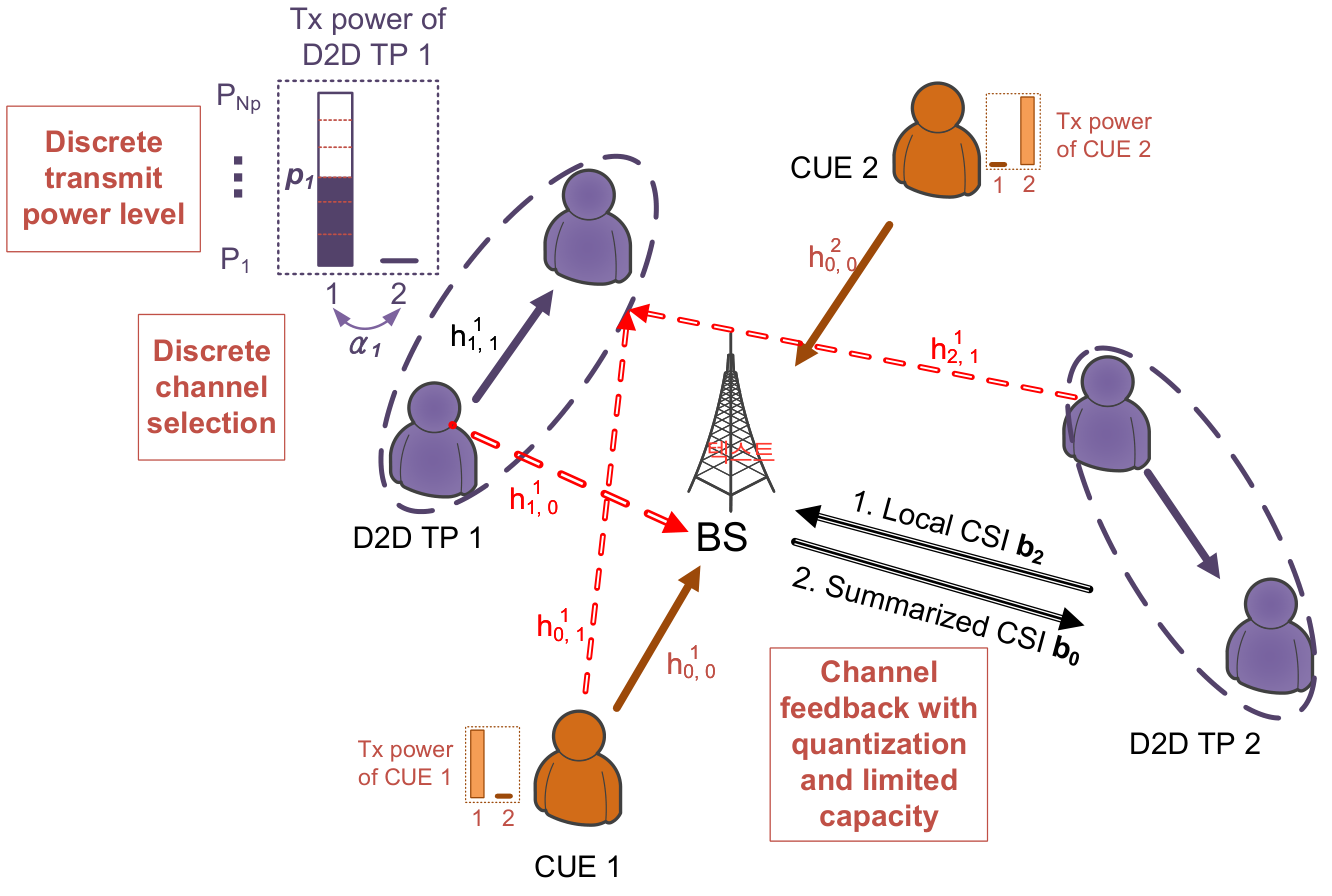
The channel gain of the -th channel, which comprises both the distance-dependent channel gain (i.e., path loss) and multipath fading, is denoted as , where and are the indices of the D2D transmitters and receivers, respectively, and and are the indices of the CUEs and the BS, respectively. For example, is the channel gain between the CUE and the receiver of the first D2D TP in the first channel, see Fig. 1. Furthermore, denotes the vector of channel gains that D2D TP can acquire, i.e., its local CSI, and is the matrix containing all , i.e., the global CSI. In addition, sets and contain all possible realization of and , , respectively.
We assume that the D2D TPs cannot utilize multiple channels simultaneously. Specifically, indicates whether D2D TP uses the -th channel, i.e., if D2D TP transmits data over channel and otherwise. Given that each D2D TP can utilize only one channel at a time, . Moreover, we define as the vector of channel usage indicators for D2D TP . Unlike in [36] and [37], where users can utilize multiple channels simultaneously, the consideration of single channel usage results in an integer programming problem, which is difficult to solve efficiently.
The transmit power of D2D TP is denoted as . We assume that the transmit power of the users is divided into discrete levels such that , where the elements of are organized in ascending order such that and . Herein, is the maximum transmit power of each user. The consideration of discrete power levels, which are used in many communication standards, e.g., 3GPP LTE and IS-95 [43, 44], is more realistic than assuming continuous power levels. Moreover, discrete power levels are beneficial when transmitters have limited capabilities due to hardware constraints, e.g., in machine-type communications [45]. However, optimization problems involving discrete power levels are more difficult to solve than problems with continuous power levels because of the resulting integer programming. Furthermore, we assume that the transmit power of the CUEs is . In addition, we denote the bandwidth of each channel and the noise power spectral density by and , respectively.
II-B Problem Statement
In this paper, the objective of resource allocation is to maximize22 2 We note that the proposed approach is general and allows the use of other objective functions, e.g., the maximization of the EE, and the incorporation of additional constraints. In Section V, we show that the proposed DNN structure can also be employed to maximize the sum EE of the D2D TPs. the sum SE of the D2D TPs while guaranteeing that the SE of the CUEs does not fall below a certain threshold, , which constitutes a QoS requirement. To this end, the selection of the channel, , and the transmit power level, , have to be optimized according to the current channel conditions.
According to the universal approximation theorem [32, 13, 42], DNNs can approximate arbitrary functions. Therefore, instead of solving the optimization problem for resource allocation for each channel realization, functions that approximate the optimal resource allocation strategy for arbitrary channel conditions can be realized via DNNs. Then, the optimal resource allocation is found by feeding the current channel gains to the DNN instead of solving the optimization problem independently for each channel realization [14, 36, 37].
Regarding the availability of CSI, we consider two cases, namely full CSI and partial CSI, which lead to centralized and distributed resource allocation policies, respectively. In the former case, the BS is able to collect the complete CSI, , such that the resource allocation for each D2D TP can be determined in a centralized manner. In the latter case, the CSI is shared via CSI feedback channels with limited capacity such that the resource allocation has to be determined in a distributed manner based on partial CSI. Moreover, for the case of partial CSI, the local CSI has to be encoded, which has to be taken into account for the optimization. In the following two subsections, we provide the detailed problem formulations for centralized and distributed resource allocation, respectively.
II-C Centralized Resource Allocation
For centralized resource allocation, full CSI is assumed to be available and our objective is to find the optimal resource allocation policy for this case. Let and denote the functions that approximate the optimal channel selection and transmit power level of D2D TP , such that and . In the considered D2D system model, the receiver of D2D TP receives data from the transmitter of D2D TP and interference from the transmitters of the other D2D TPs and the CUE. Accordingly, the achievable SE of D2D TP in the -th channel, , with resource allocation policy and is given as follows:
| (1) |
where corresponds to the interference from the CUE using channel .
Similarly, the SE of the CUE using channel , which we denote by , can be written as follows:
| (2) |
Then, the functions and , which maximize the overall SE of the D2D TPs subject to a minimum required SE of the CUE, , can be found by solving the following optimization problem:
| (3) |
In (3), the expected SE is maximized instead of the instantaneous SE since functions, and , which are optimal for any given channel condition, , are designed.
II-D Distributed Resource Allocation
For distributed resource allocation, the local CSI is shared among the D2D users, and then each D2D user determines its own resource allocation in a distributed manner based on the collected partial CSI. Accordingly, the sharing of local CSI needs to be optimized along with the resource allocation. Herein, considering how CSI is acquired in existing cellular communication standards, e.g., 3GPP LTE [46, 47], we assume that each D2D user sends the local CSI to the BS first, and then the BS broadcasts the collected CSI to the D2D users. Although the direct sharing of local CSI among users has been considered in the literature [34, 42], it can cause a huge signaling overhead and some D2D users may not be able to share their local CSI because of the large distances between them.
For distributed resource allocation, we assume that the capacity of the CSI feedback channel is limited such that each D2D TP compresses its local CSI to bits and sends the compressed local CSI to the BS, see Fig. 1. The local CSI reported by D2D TP to the BS is denoted as . The encoding of the local CSI is modeled via function for given local CSI such that . Then, the BS accumulates the local CSI from all D2D TPs, , and broadcasts the collected local CSI and its own CSI, , to all D2D TPs, where the broadcast CSI is compressed into bits by the BS. The CSI sent from the BS to all D2D TPs is denoted by and determined by function for given local CSI of the channel of the CUE at the BS, , and encoded local CSI of the D2D TPs, , such that . Note that the total signaling overhead for distributed resource allocation is bits because each D2D TP reports its own local CSI using bits and the BS broadcasts the accumulated local CSI to the D2D TPs using bits.
Accordingly, for distributed resource allocation, the optimal encoding strategies for local CSI sharing, i.e., and , have to be determined. In addition, the optimal resource allocation strategy of the D2D TPs has to be obtained based on local CSI, , and the combined CSI sent by the BS, . Let and be the functions that model the channel selection and the transmit power level of D2D TP for partial CSI, such that and .
Then, the following optimization problem must be solved for distributed resource allocation:
| (4) |
where and are given as follows
| (5) |
Since the resource allocation strategies of all D2D TP need to be jointly optimized to achieve the common goal of maximizing the sum SE, a centralized optimization problem is formulated in (4), i.e., the strategies for channel and transmit power level selection for each D2D TP are jointly derived. However, each D2D TP can determine its resource allocation strategy individually solely based on local CSI and the summarized CSI coming from the BS , because and are the functions of and .
III DNN Structure For Deep Learning Based Resource Allocation
In this section, we present the proposed DNN structure used to approximate the optimal resource allocation functions for centralized and distributed resource allocation, i.e., , , , , , and .
III-A Structure of Basic DNN Module
In this subsection, we describe the basic DNN module which constitutes the basic building block of the proposed DNNs. The basic DNN module is composed of multiple basic units which are in turn composed of one fully connected (FC) layer, one batch normalization (BN) layer, one rectified linear unit (ReLU) layer, and one dropout layer, as depicted in Fig. 2. These basic DNN modules are used to approximate functions, , , , , , and .
In the FC layer, the output is determined by the multiplication of weights and the addition of a bias to the input [38, 48]. Let , , and denote the input vector, weight matrix, and bias vector of the FC layer, respectively. Then, the output is given by .
The output of the FC layer is fed into the BN layer which performs mini batch-wise normalization [48, 49]. In general, during the training of DNNs, multiple input data, i.e., mini batches, are fed into the DNN simultaneously in order to reduce the computation time via parallel processing. In the BN layer, mini batch data is normalized by its own mean and variance. Then, the normalized data is multiplied by weights and biases are added whose values are adjusted during training. Mathematically, let be the input of the BN layer, then the output of the BN layer is given by , where and are the weight and bias of the BN layer, and is a small constant to prevent division by zero. Moreover, and . It has been shown that the use of a BN layer is an effective means to avoid the overfitting problem and the vanishing gradient problem in DNNs by regulating the distribution of the inputs of the subsequent layers [49].
Then, the output of the BN layer is fed into the ReLU layer which introduces nonlinearity to the DNN [50, 38]. Specifically, for input vector , the output of the ReLU layer is , i.e., negative inputs are blocked by the ReLU layer. The use of ReLU is also beneficial in view of computation time because its output and derivative are very easy to calculate.
Finally, the dropout layer is applied to the output of the ReLU layer. In the dropout layer, the input data is randomly dropped with a certain probability such that some of the input data is blocked from being forwarded to the subsequent layer. This drop out is an efficient regularization technique to avoid the overfitting of DNNs [14].
The proposed basic DNN module is composed of basic units which are sequentially connected, cf. Fig. 2. The numbers of inputs and outputs of a basic DNN module are denoted by and , respectively. Moreover, the number of hidden nodes of each basic unit, which corresponds to the size of the FC layer, is given by , except for the last basic unit, whose number of hidden nodes is equal to the number of outputs of the basic unit, i.e., . Furthermore, inspired by recent advances in DL, we consider residual connections (short-cut connections) in the basic DNN module, such that the output of the first basic unit is forwarded to the subsequent units via short-cut connections [51]. More specifically, the output of the first basic unit is added to the output of the BN layer of the subsequent units. These residual connections can help in the training of the DNN [51].
III-B Structure of Centralized DNN Model
In this subsection, we present the structure of the centralized DNN model which is used to determine the resource allocation based on full CSI, cf. Fig. 3. In the centralized DNN model, the complete CSI, , is applied as input and the transmit power level, , and the channel selection, , are the outputs. Moreover, the centralized DNN model is implemented at the BS, which collects the CSI from the users and informs the resource allocation to each D2D TP. First, the input is pre-processed by converting it to the dB scale and normalized to have zero mean and unit variance which facilitates proper training of the DNN [14]. The dB scale is preferable compared to the decimal scale due to the reduced range of possible channel gains.
Let be the matrix of pre-processed channel gains. The elements of , which are denoted by , are given as follows:
| (6) |
After pre-processing of the data, is reshaped into a one-dimensional vector of length , and then fed into two separate basic DNN modules, which are the basic DNN module for the transmit power level (BDP) and the basic DNN module for the channel selection (BDC). The BDP and BDC modules independently determine the transmit power level and channel selection, respectively, i.e., they are used to approximate functions and .
The number of outputs of the BDP module, which calculates the transmit power levels of all D2D TPs, is . The outputs of the BDP module are divided into groups, where each group contains elements, respectively. Then, each group of outputs is fed into separate softmax layer blocks, which perform the softmax operation, such that when the input of the -th softmax layer block is , the -th output of the -th softmax layer block becomes [48]. The output of the -th softmax layer block, which we denote as , specifies the probabilities with which each transmit power level is selected, i.e., the -th element of corresponds to the probability that D2D TP uses transmit power level, .
The determination of the transmit power level for D2D TP is different for training and inference. During training, the transmit power level of D2D TP is determined by the multiplication of and the discrete transmit power levels. Mathematically, , where is the -th element of . On the other hand, during inference when the D2D TP actually uses the trained DNN to determine its transmit power, cannot be used because the constraint can be violated. Instead, the index of which corresponds to the largest value is employed to select the transmit power level, such that where . Note that the used during training is differentiable, and hence, back-propagation based training can be used. However, the used during inference cannot be used for training because is not differentiable.
The structure of the BDC module, which determines the channel selection, is almost identical to that of the BDP module except that the outputs of the softmax layer directly determine the channel selection . First, the reshaped channel gain is fed into the BDC module which has outputs. Then, the outputs of the BDC module are divided into groups which are fed into independent softmax layer blocks whose outputs are . To be more specific, the -th output of the -th softmax layer block can be interpreted as the probability that D2D TP selects channel . Similar to the determination of the transmit power level, the determination of the channel selection is different for training and inference. Specifically, during training, the output of the BDC module, , is directly used as the channel selection while during inference, we set for and for all other such that the constraint is satisfied in the actual implementation. Hence, due to this binarization, the resource allocation strategy employed during training may differ from that used for inference, which leads to performance deterioration. Thus, during the training process, the deviation of and from binary values is penalized, see Section IV, such that the binarization error is reduced to zero.
III-C Structure of Distributed DNN Model
In this subsection, we provide a detailed description of the structure of the distributed DNN model which relies only on partial CSI. The complete structure of the distributed DNN model is depicted in Fig. 4. Unlike the centralized case, where a single DNN module determines the resource allocation of all D2D TPs, in the distributed case, each D2D TP uses a different DNN module with the corresponding local CSI, , and summarized CSI, , as its input. Accordingly, the DNN module which determines , , and is implemented at the D2D TP , , while the DNN module that determines is implemented at the BS.
First, the local CSI is converted to the dB scale and normalized to have zero mean and unit variance, similar as for the centralized DNN structure. Let vector contain the pre-processed channel gains of D2D TP . Then, is fed into the basic DNN module for CSI feedback (BDF), which has outputs and determines the encoded CSI that is sent to the BS, i.e., . The BDF module is followed by a sigmoid layer which converts input to output . The BDF module and sigmoid layer together approximate the function for the encoding of the local CSI, . Given that all outputs of the BDF module are subject to separate sigmoid operations, the total number of outputs is , which is identical to the number of bits allocated for local CSI sharing. Unlike for the transmit power level and channel selection, for , multiple output values can have a value of 1, which is the reason for employing a sigmoid layer instead of a softmax layer.
After D2D TP has determined , this compressed CSI is sent to the BS and is merged to determine the encoded CSI which is broadcast back to all D2D TPs. To this end, the encoded CSI received from the D2D TPs and the local BS CSI are fed together into the basic DNN module for CSI notification (BDN) which determines , i.e., the BDN module approximates . The output of the BDN module is fed into a sigmoid layer to obtain which is then sent back to each D2D TP. Note that the output of all sigmoid layers, i.e., BDF and BDN, is forced to become either 0 or 1 during training to ensure proper binarization as explained in Section IV.
Upon receiving from the BS, each D2D TP independently determines its transmit power level and channel selection based on its local CSI, , and the summarized global CSI received from the BS, , using the BDP and BDC modules, as for the centralized DNN model. However, unlike for the centralized DNN model, where softmax layer blocks are used, only one softmax layer block is used for each D2D TP because the transmit power level and the channel selection for only one D2D TP are determined.
IV Training and Inference of the Proposed DNN Models
In this section, we first explain the training methodology of the proposed DNN models and the corresponding loss functions. Then, we discuss how trained DNNs can be used to determine the resource allocation, i.e., the inference of the DNN.
IV-A Training of the Proposed DNN Models
In the proposed scheme, the constructed DNN models must be trained first, before they are used to allocate the wireless resources for the D2D TPs. We employ off-line training33 3 In this paper, off-line training is employed because training the DNN models is time consuming and the speed of training can be improved through the use of the parallel computing. However, both the BS and the D2D TPs are unlikely to have this capability., i.e., the DNN models are trained on an independent computation unit and the parameters of trained DNN models are forwarded to the BS and D2D TPs. Herein, we adopt a hybrid training strategy exploiting both supervised and unsupervised learning [14]. Specifically, the DNN models are first trained using a supervised learning strategy based on a few channel samples and the corresponding optimal resource allocation strategies.
This is referred to as coarse tuning (CT), i.e., the DNN models are trained to mimic the optimal resource allocation policies which are given as a label data. After CT, a unsupervised learning strategy based on a large number of channel samples, which we refer to as fine tuning (FT), is applied to the DNNs which have been already trained via CT. During FT, the weighted sum of objective functions and the constraints in (3) and (4) are used as loss function. During both CT and FT, stochastic gradient descent algorithms, e.g., Adam (Adaptive Moment Estimation) [14], are used to update the weights of the DNNs.
The main rationale behind using the proposed hybrid training strategy is to combine the benefits of both individual training strategies, the optimality of supervised learning and the avoidance of label data for unsupervised learning. More specifically, in unsupervised learning, the optimal resource allocation policy has to be found through trial-and-error and the algorithm may converge to a wrong policy. However, in supervised learning, the DNN is simply trained to mimic the provided optimal resource allocation, such that the optimal resource allocation policy can always be obtained. However, the acquisition of the labels needed for supervised learning is time consuming because the label data, i.e., the optimal resource allocation, has to be found through an exhaustive search, while unsupervised learning only requires CSI for training.
In order to balance the trade-off between these two training strategies, in our proposed scheme, the DNN is first trained using CT, and then FT is used to finely tune the weights of the DNN models. Indeed CT can be considered as the initialization before the actual training starts, such that the weights of the DNN are adjusted to favorable initial values before FT is performed. As a result, the training time of the DNN for FT is reduced compared to the case without CT, as can be observed from the simulation results provided in Section V. Note that during CT, a small dataset is utilized in order to reduce the overhead introduced by computing the optimal resource allocation policy, which is needed as a label data during CT.
IV-B Loss Functions for Training
During the CT phase, the DNN is trained to mimic the optimal channel and transmit power level selection, which we denote as and , respectively, where only when is selected as desired power level. Note that and can be obtained through exhaustive search. Then, the DNN models are trained to minimize loss functions, and , for the centralized and distributed DNN models, respectively. The loss functions are given by
| (7) |
where , , and are control parameters which have to be positive. Furthermore, , , and in (7) are defined as follows:
| (8) |
where is a control parameter which has to be positive.
In (7), corresponds to the cross entropy loss such that the value of the loss function is minimized when the outputs of the DNN, i.e., and , are identical to the given label data, and . Subsequently, the DNN model is trained to make and identical to the given optimal resource allocation, i.e., and . We note that the use of the cross entropy loss function can improve the training speed [48] compared to the mean squared error loss function used in [13]. Moreover, and are the binarization errors of the transmit power level and channel selection, i.e., and . Similarly, is the binarization error for the CSI encoding, i.e., . Given that the values of , , and decrease as the , , and approach either 0 or 1, the training pushes the values of , , and towards binary values44 4 For the binarization techniques considered in [27, 52], a sigmoid function with steep slope is employed. This can possibly affect the performance of back-propagation based training because the gradient of a sigmoid function with steep slope is likely to be 0 for most input values. In our proposed scheme, by adopting a polynomial function in the loss function, the problem of vanishing gradient is avoided since the gradient of polynomial function is likely to be non-zero for all possible and .. We note that the BDF, BDN, BDP, and BDC modules of the distributed DNN model are jointly trained because the output of one module affects the other modules.
Next, we present the loss functions of the centralized and the distributed DNN models during the FT phase, and , which are given as follows:
| (9) |
where , , , , and are positive control parameters and is a small positive constant which prevents division by zero when .
In (9), the first term corresponds to the negative objective function used for resource allocation, namely, sum SE of the D2D TPs. The value of the loss function decreases when the sum SE of the D2D TPs increases. Moreover, the second term in (9) depends on how much the QoS constraint for legacy cellular uplink transmission is violated, i.e., . Accordingly, the value of the loss function increases when the QoS constraint is not satisfied. As a result, the DNNs can be trained when the optimal resource allocation is not available as label data. Moreover, as in (7), , , and are used for binarization. Note that the values of , , , , and determine whether the DNN model puts more emphasis on the maximization of the SE, meeting the QoS constraint, or the binarization of the output of the DNN.
Remark 1 Although the proposed loss functions in (9) are different from the conventional loss functions typically used for DL, e.g., the cross entropy loss, the back propagation based training of the DNN is still applicable because the proposed loss functions are differentiable [53].
Remark 2 The proposed DNN model can cope with different design objectives and constraints easily by modifying the loss function. For example, the DNN model can be trained to maximize the EE by replacing in (9) by , which is given by , where is the circuit power consumption of the D2D users.
Remark 3 In the proposed scheme, the training is performed before the DNNs are employed in the communication system, i.e., in an off-line manner. Hence, the overhead incurred during training of the DNNs, which can be huge, is not an obstacle for real-time operation of the proposed scheme [14, 36, 38, 37].
IV-C Inference of the Proposed DNN Model
The transmit power level (), channel selection (), and CSI feedback (, ) can be determined by feeding the current channel gains to the trained DNN models. Given that the proposed DNN models involve only simple matrix calculations and functions, the optimal resource allocation policy can be determined fast even when the number of users and channels is large, as will be confirmed later in Section V.
V Performance Evaluation
In this section, we assess the performance of the proposed DL-based resource allocation scheme. We assume that the users are randomly distributed over a 100 m 100 m area, where the maximum distance between a transmitter and a receiver in the same TP is set to 30 m. Moreover, we assume that = 23 dBm and = 8, i.e., the transmit power is equally divided into 8 levels. Accordingly, , mW mW, mW, mW, mW, mW, and mW. Furthermore, , ,55 5 In the default simulation environment, we have considered small and due to the excessive computation time needed to determine the optimal performance via exhaustive search even for moderate values of and , see Fig. 11. 10 MHz, = -173 dBm/Hz, = 12, and = 24, such that the CSI is compressed to 12 bits and 24 bits for the D2D TPs and the BS, respectively. A simplified path loss model with path loss coefficient and path loss exponent is adopted [14]. The small-scale fading gains are modeled as independent and identically distributed (i.i.d.) circularly symmetric complex Gaussian (CSCG) random variables with zero mean and unit variance. Furthermore, we assume that and channel samples are generated for training and evaluation, respectively. In addition, Adam [54] is used for training where the learning rate, which determines the speed of learning, is set to and for the CT and FT phases, respectively.
Regarding the structure of the DNN model, for the centralized DNN model, we assume that the numbers of hidden layers and hidden nodes for both the BDP and BDC modules are 16 and 400, respectively. Moreover, for the distributed DNN model, the numbers of hidden layers and hidden nodes of the BDF, BDN, BDP, and BDC modules are set to 8 and 150, respectively. Furthermore, the values of the control parameters for the QoS constraint and binarization, i.e., , , , , , , , and are adaptively determined for each simulation environment through trial-and-error. For performance evaluation, three conventional schemes are considered, namely 1) the optimal scheme, 2) the naive distributed DL-based scheme proposed in [14], and 3) a random scheme. For the optimal scheme, the optimal resource allocation policy is found through exhaustive search. For our default simulation setting, where = 8, , and , the total number of possible resource allocation strategies is 10648, all of which have to be examined in the exhaustive search. For the naive scheme, the centralized DNN model, which is trained based on the complete CSI, is used for distributed operation, where the average values of the non-local CSI values are employed to determine the resource allocation. For the random scheme, the channel and transmit power levels are randomly selected.

First, in order to confirm the benefits of the proposed hybrid training strategy, where CT is used as a means to initialize the DNN, we evaluate the evolution of the loss functions for FT, and , by varying the proportion of samples used for CT, , as depicted in Fig. 5, where an epoch is the number times that the entire training dataset is used for training. As can be observed from Fig. 5, the speed of convergence can be greatly improved by employing CT, even when only a small fraction of samples is used for CT, i.e., , which demonstrates the usefulness of CT. Moreover, for the distributed DNN model, more time is required for training than for the centralized DNN model because the encoding of the CSI has to be also optimized in addition to the resource allocation. We note that the training time required for CT is negligible because the amount of training data is small. For example, for , CT takes 0.04 seconds while FT takes more than 60 seconds for one epoch of training.


In Figs. 6 and 7, we show the cumulative distribution function (CDF) of the SE of the D2D TPs and the CUEs for different . For the calculation of the SE, we set the SE of the D2D TPs to zero when the QoS constraint is not satisfied in order to penalize the QoS violation. From the simulation results, we observe that the SE of the D2D TPs deteriorates while that of the CUEs improves when increases because the transmit power of the D2D TPs is more severely regulated when is larger in order to meet the QoS constraints of the CUEs. As can be observed from the results in Fig. 6, the performance of DNN-based resource allocation is almost identical to that of the optimal scheme when . Although the SE of the D2D TPs for the proposed scheme is slightly degraded when 1 b/s/Hz, it is much higher than that obtained for the naive and random schemes. Furthermore, we observe that the SE of the D2D TPs is slightly lower for the distributed DNN model than for the centralized DNN model, because for the distributed scheme, only partial CSI is employed. In addition, the random scheme has the worst SE for the D2D TPs and the CUEs in all cases, which underscores the need for a proper resource allocation optimization.


The naive scheme yields a poor SE for the D2D TPs, especially when = 1 b/s/Hz. This is mainly due to high probability that the QoS constraint is violated66 6 The violation of the QoS constraint is obvious from the starting point of the CDF of the SE of the CUEs in Fig. 7. More specifically, the CDF of the optimal scheme starts at such that the SE of the CUEs is always larger than . On the other hand, the CDF of the other schemes starts at a point which is smaller than such that some CUEs will achieve a lower SE than , i.e., the QoS constraint is violated. We note that the starting point of the CDF of the proposed scheme is much closer to that of the optimal scheme compared to the other schemes, i.e., the QoS constraint is almost always satisfied. for the naive scheme. This probability can be as high as 32% when = 1 b/s/Hz, cf. Fig. 9(b). We note that for the proposed centralized and distributed DNN-based schemes, the QoS violation probability is less than 2.7%, which validates the usefulness of the proposed design, see Fig. 9(b). Moreover, we observe that although the QoS constraint may be violated for some channel realization for the proposed scheme, the overall SE of the CUEs is increased compared to the optimal scheme, cf. Fig. 7. This behavior is due to the fact that the proposed scheme restricts the transmit power of the D2D TPs more severely such that the overall SE of the D2D TPs is slightly degraded but that of the CUEs is slightly increased compared to the optimal scheme.
In order to confirm that the outputs of the DNNs are properly binarized, we consider the CDF of the binarization error defined as , where denotes the nearest integer value for = 1 b/s/Hz. The CDF of the errors for the transmit power level and channel selection are shown in Fig. 8(a) and those for (CSI from D2D TP 1), (CSI from D2D TP 2), (CSI from D2D TP 3), and (CSI from BS) are depicted in Fig. 8(b). Given that these optimization variables are in the range between 0 and 1, the maximum value of the binarization error is 0.5. From Fig. 8, we observe that the binarization error for all optimization variables is negligibly small, which confirms that our DNN models are able to generate binary values.


Next, we show the average SE of the D2D TPs, the probability of QoS constraint violation, and the level of QoS violation, which is defined as the difference between the QoS requirement and the SE of the CUEs when the QoS constraint is violated, i.e., , as a function of in Figs. 9(a) - 9(c). As can be observed from Fig. 9(a), the average SE of the D2D TPs decreases as increases because the transmit power and channel usage of the D2D TPs have to be restricted more severely in order to satisfy the QoS constraints of the CUEs. Moreover, we observe that the average SE of the proposed scheme is slightly degraded compared to the optimal scheme while the gap between both schemes decreases for small . In Fig. 9(b), we observe that the QoS violation probability of the proposed schemes is close to 0 while that of the conventional schemes is much higher, which highlights the effectiveness of the proposed scheme. Moreover, from Fig. 9(c), we observe that the level of QoS violation for the proposed scheme is small such that even though the QoS constraint is violated, the SE of the CUEs is likely very close to such that the impact of the QoS violation is minimal.


In Figs. 10(a) - 10(c), we show the average SE of the D2D TPs, the probability of QoS constraint violation, and the level of QoS violation as a function of the number of D2D TPs, . Because of the excessive computation time needed to determine the performance of the optimal scheme for large , the performance of the optimal scheme is not shown. As can be seen from Fig. 10(a), the average SE of the D2D TPs decreases as increases due to the increased interference among the D2D TPs. Moreover, the naive scheme and the random scheme yield worse performance compared to the proposed scheme in terms of the average SE. In fact, the average SE of the random scheme approaches zero as the number of D2D TPs increases due to the high probability of QoS violation, as confirmed by Fig. 10(b). Furthermore, Fig. 10(c) shows that the level of QoS violation of the proposed scheme increases as increases due to the fixed size of the DNN. Specifically, since we have used a relatively small DNN structure for both the centralized and distributed DNN schemes, the ability of the DNNs to approximate arbitrary functions is not high. However, the dimensionality of the resource allocation strategy increases for larger , such that the performance of the proposed scheme deteriorates in this case.
Next, in Fig. 11, we compare the computation time77 7 For these simulation results, only the computation time for the inference phase is measured because the training of the DNN can be performed off-line before its actual usage. needed for resource allocation as a function of , where the computation time is measured using an Intel Core i7-7700k running at 4.2 GHz with 64 GB of memory, and the simulation codes are implemented using Python 3.7 and Tensorflow 2.0.0. For a fair comparison, parallel computation, which can further reduce the computation time of DNN-based schemes, is not employed. From the results in Fig. 11, we observe that the computation time of the optimal scheme increases exponentially with , and when , the computation time to find the optimal resource allocation policy for one channel sample exceeds 25.9 hours, which is far too high for practical systems. On the other hand, the computation time of the proposed scheme does not increase significantly with . For , the computation times for the centralized and distributed DNN schemes are equal to 1.6 and 24 milliseconds (not shown in Fig. 11), respectively. This suggests that the proposed scheme is applicable even for large number of users. Furthermore, we observe that the computation time of the distributed DNN scheme is larger than that of the centralized DNN scheme due to the additional binarization of the CSI.

To illustrate the encoding of the CSI, the value of as a function of the normalized channel gain is shown in Fig. 12 where is encoded by 2 bits for simplicity of presentation. In this simulation, the number of D2D TPs and the number of channels are assumed to be 2 and 1, respectively, and the normalized channel gains , , and are denoted as , and , respectively, in order to simplify the interpretation of the results. Note that corresponds to the channel gain of the CUE and and correspond to the gains of the interfering channels such that the rate of the CUE is likely large when is high and and are small. As can be observed from Fig. 12, the value of is carefully designed by the DNN to reflect the channel conditions such that a given represents similar channel conditions. For example, when the channel gain of the CUE is small and the interference from D2D TP 1 is large, is likely to be encoded to . This result verifies the efficiency of the proposed DNN-based approach for CSI representation.

Finally, in Fig. 13, we show the performance of the proposed scheme for maximizing the overall EE of the D2D TPs, i.e., , where . In the simulation, we assume that the circuit power of the D2D TPs, , is 500 mW and = 0 b/s/Hz [55]. To maximize the overall EE, we replaced the SE in the loss functions of the proposed schemes by the corresponding EE. From Fig. 13, we observe that the proposed scheme also achieves a close-to-optimal performance in this case and outperforms the conventional non-optimal schemes. The simulation results in Fig. 13 confirm the versatility of the proposed scheme in coping with different design objectives.
VI Conclusions
In this paper, we studied the resource allocation algorithm design for multi-channel cellular networks with D2D communication using a DL framework. We focused on the maximization of the overall SE of the D2D TPs while guaranteeing a minimum data rate for the legacy cellular users. Our problem formulation takes into account discrete optimization variables, namely channel selection and discrete transmit power levels. In addition, we considered both a centralized and a distributed approach for resource allocation. In the latter case, encoded CSI is exchanged between the D2D users and the BS via limited feedback channels. We designed centralized and distributed DNN models that approximate both the optimal resource allocation strategy and the optimal encoding strategy of the local CSI for a limited feedback capacity. In order to facilitate the training of the proposed DNN models, a hybrid supervised and unsupervised learning strategy with novel loss functions was devised and shown to enable efficient training based on a few ground-truth labels. Through computer simulations, we confirmed that the proposed resource allocation schemes achieve near-optimal performance with low computation time, which underlines their applicability in practical systems. Specifically, we found that the distributed resource allocation scheme achieves a similar performance as the centralized scheme, which validates the effectiveness of the proposed CSI representation using a DNN. Furthermore, we verified the scalability of the proposed schemes for a large number of users in view of computation time and showed that the proposed DNN model can be applied to achieve various design objectives, e.g., EE maximization.
References
- [1] D. W. K. Ng, E. S. Lo, and R. Schober, “Multiobjective resource allocation for secure communication in cognitive radio networks with wireless information and power transfer,” IEEE Trans. Veh. Technol., vol. 65, no. 5, pp. 3166–3184, May 2015.
- [2] M. El Tanab and W. Hamouda, “Resource allocation for underlay cognitive radio networks: A survey,” IEEE Commun. Surveys Tuts., vol. 19, no. 2, pp. 1249–1276, 2016.
- [3] K. Lee, C. Yoon, O. Jo, and W. Lee, “Joint optimization of spectrum sensing and transmit power in energy harvesting-based cognitive radio networks,” IEEE Access, vol. 6, pp. 30 653–30 662, Jun. 2018.
- [4] C.-H. Yu, K. Doppler, C. Ribeiro, and O. Tirkkonen, “Resource sharing optimization for device-to-device communication underlaying cellular networks,” IEEE Trans. Wireless Commun., vol. 10, no. 8, pp. 2752–2763, Aug. 2011.
- [5] Y. Jiang, Q. Liu, F. Zheng, X. Gao, and X. You, “Energy-efficient joint resource allocation and power control for D2D communications,” IEEE Trans. Veh. Technol., vol. 65, no. 8, pp. 6119–6127, Aug. 2016.
- [6] W. Lee, T. Ban, and B. C. Jung, “Distributed transmit power optimization for device-to-device communications underlying cellular networks,” IEEE Access, vol. 7, pp. 87 617–87 633, Jul. 2019.
- [7] G. Fodor and N. Reider, “A distributed power control scheme for cellular network assisted D2D communications,” in Proc. of Globecom, Houston, TX, Dec. 2011.
- [8] S. Pyun, W. Lee, and D. Cho, “Resource allocation for Vehicle-to-Infrastructure communication using directional transmission,” IEEE Trans. Intell. Transp. Syst., vol. 17, no. 4, pp. 1183–1188, Apr. 2016.
- [9] J. Gao, M. R. A. Khandaker, F. Tariq, K. Wong, and R. T. Khan, “Deep neural network based resource allocation for V2X communications,” in Proc. of VTC2019-Fall, Honolulu, HI, USA, Sep. 2019.
- [10] Y. Sun, D. W. K. Ng, Z. Ding, and R. Schober, “Optimal joint power and subcarrier allocation for MC-NOMA systems,” in Proc. of Globecom, Washington, DC, USA, Dec 2016.
- [11] X. Li, C. Li, and Y. Jin, “Dynamic resource allocation for transmit power minimization in OFDM-based NOMA systems,” IEEE Commun. Lett., vol. 20, no. 12, pp. 2558–2561, Dec 2016.
- [12] Q. Shi, M. Razaviyayn, Z. Q. Luo, and C. He, “An iteratively weighted MMSE approach to distributed sum-utility maximization for a MIMO interfering broadcast channel,” IEEE Trans. Signal Process., vol. 59, no. 9, pp. 4331–4340, Sep. 2011.
- [13] H. Sun, X. Chen, Q. Shi, M. Hong, X. Fu, and N. D. Sidiropoulos, “Learning to optimize: Training deep neural networks for interference management,” IEEE J. Sel. Topics Signal Process., vol. 66, no. 20, pp. 5438–5453, Oct. 2018.
- [14] W. Lee, M. Kim, and D. H. Cho, “Deep power control: Transmit power control scheme based on convolutional neural network,” IEEE Commun. Lett., vol. 22, no. 6, pp. 1276–1279, Jun. 2018.
- [15] Y. LeCun, Y. Bengio, and G. Hinton, “Deep learning,” Nature, vol. 521, no. 7553, pp. 436–444, May 2015.
- [16] T. Wang, C.-K. Wen, H. Wang, F. Gao, T. Jiang, and S. Jin, “Deep learning for wireless physical layer: Opportunities and challenges,” China Communications, vol. 14, no. 11, pp. 92–111, Nov. 2017.
- [17] H. Ye, G. Y. Li, and B. H. Juang, “Power of deep learning for channel estimation and signal detection in OFDM systems,” IEEE Wireless Commun. Lett., vol. 7, no. 1, pp. 114–117, Feb. 2018.
- [18] X. Cheng, D. Liu, C. Wang, S. Yan, and Z. Zhu, “Deep learning-based channel estimation and equalization scheme for FBMC/OQAM systems,” IEEE Wireless Commun. Lett., vol. 8, no. 3, pp. 881–884, Jun. 2019.
- [19] N. Samuel, T. Diskin, and A. Wiesel, “Deep MIMO detection,” in Proc of SPAWC, Sapporo, Japan, Jul. 2017.
- [20] H. He, C. Wen, S. Jin, and G. Y. Li, “Deep learning-based channel estimation for beamspace mmWave massive MIMO systems,” IEEE Wireless Commun. Lett., vol. 7, no. 5, pp. 852–855, Oct. 2018.
- [21] N. Farsad and A. Goldsmith, “Neural network detectors for molecular communication systems,” in Proc. of IEEE SPAWC, Kalamata, Greece, Jun. 2018.
- [22] A. Klautau, N. González-Prelcic, A. Mezghani, and R. W. Heath, “Detection and channel equalization with deep learning for low resolution MIMO systems,” in Proc. of Asilomar Conference on Signals, Systems, and Computers, Pacific Grove, CA, USA, Oct. 2018.
- [23] C. Wen, W. Shih, and S. Jin, “Deep learning for massive MIMO CSI feedback,” IEEE Wireless Commun. Lett., vol. 7, no. 5, pp. 748–751, Oct. 2018.
- [24] T. J. O’Shea, J. Corgan, and T. C. Clancy, “Convolutional radio modulation recognition networks,” in Proc. of EANN, Aberdeen, U.K., Sep. 2016.
- [25] T. J. O’Shea, S. Hitefield, and J. Corgan, “End-to-end radio traffic sequence recognition with recurrent neural networks,” in Proc. of GlobalSIP, Washington, DC, USA, Dec. 2016.
- [26] W. Lee, M. Kim, and D. Cho, “Deep cooperative sensing: Cooperative spectrum sensing based on convolutional neural networks,” IEEE Trans. Veh. Technol., vol. 68, no. 3, pp. 3005–3009, Mar. 2019.
- [27] H. Lee, S. H. Lee, T. Q. S. Quek, and I. Lee, “Deep learning framework for wireless systems: Applications to optical wireless communications,” IEEE Commun. Mag., vol. 57, no. 3, pp. 35–41, Mar. 2019.
- [28] M. Kim, N. I. Kim, W. Lee, and D. H. Cho, “Deep learning aided SCMA,” IEEE Commun. Lett., vol. 22, no. 4, pp. 720–723, Apr. 2018.
- [29] T. J. O’Shea, T. Roy, and T. C. Clancy, “Over-the-air deep learning based radio signal classification,” IEEE J. Sel. Topics Signal Process., vol. 12, no. 1, pp. 168–179, Feb. 2018.
- [30] S. Dörner, S. Cammerer, J. Hoydis, and S. t. Brink, “Deep learning based communication over the air,” IEEE J. Sel. Topics Signal Process., vol. 12, no. 1, pp. 132–143, Feb. 2018.
- [31] M. Kim, W. Lee, J. Yoon, and O. Jo, “Toward the realization of encoder and decoder using deep neural networks,” IEEE Commun. Mag., vol. 57, no. 5, pp. 57–63, May 2019.
- [32] K. Hornik, M. Stinchcombe, and H. White, “Multilayer feedforward networks are universal approximators,” Neural Networks, vol. 2, no. 5, pp. 359–366, 1989.
- [33] X. Tan, Z. Zhong, Z. Zhang, X. You, and C. Zhang, “Low-complexity message passing MIMO detection algorithm with deep neural network,” in Proc. of GlobalSIP, Anaheim, CA, USA, Nov. 2018, pp. 559–563.
- [34] P. de Kerret, D. Gesbert, and M. Filippone, “Team deep neural networks for interference channels,” in Proc. of ICC Workshops, Kansas City, MO, USA, May 2018.
- [35] F. Liang, C. Shen, W. Yu, and F. Wu, “Towards optimal power control via ensembling deep neural networks,” IEEE Trans. Commun., vol. 68, no. 3, pp. 1760–1776, Mar. 2020.
- [36] W. Lee, “Resource allocation for multi-channel underlay cognitive radio network based on deep neural network,” IEEE Commun. Lett., vol. 22, no. 9, pp. 1942–1945, Sep. 2018.
- [37] W. Lee, O. Jo, and M. Kim, “Intelligent resource allocation in wireless communications systems,” IEEE Commun. Mag., vol. 58, no. 1, pp. 100–105, Jan. 2020.
- [38] W. Lee, M. Kim, and D. Cho, “Transmit power control using deep neural network for underlay device-to-device communication,” IEEE Wireless Commun. Lett., vol. 8, no. 1, pp. 141–144, Feb. 2019.
- [39] T. Van Chien, T. N. Canh, E. Björnson, and E. G. Larsson, “Power control in cellular massive MIMO with varying user activity: A deep learning solution,” IEEE Trans. Wireless Commun., vol. 19, no. 9, pp. 5732–5748, Sep. 2020.
- [40] L. Sanguinetti, A. Zappone, and M. Debbah, “Deep learning power allocation in massive MIMO,” in Proc. of Asilomar Conference on Signals, Systems, and Computers, Pacific Grove, CA, USA, Oct. 2018.
- [41] A. Zappone, M. Di Renzo, M. Debbah, T. T. Lam, and X. Qian, “Model-aided wireless artificial intelligence: Embedding expert knowledge in deep neural networks towards wireless systems optimization,” IEEE Veh. Technol. Mag., vol. 14, no. 3, pp. 60–69, Sep. 2019.
- [42] H. Lee, S. H. Lee, and T. Q. S. Quek, “Deep learning for distributed optimization: Applications to wireless resource management,” IEEE J. Sel. Areas Commun., vol. 37, no. 10, pp. 2251–2266, Oct. 2019.
- [43] H. Nguyen and W. Hwang, “Distributed scheduling and discrete power control for energy efficiency in multi-cell networks,” IEEE Commun. Lett., vol. 19, no. 12, pp. 2198–2201, Dec. 2015.
- [44] C. Liu, B. Rong, and S. Cui, “Optimal discrete power control in Poisson-clustered ad hoc networks,” IEEE Trans. Wireless Commun., vol. 14, no. 1, pp. 138–151, Jan. 2015.
- [45] M. Suciu, T. Šolc, L. Cremene, M. Mohorčič, and C. Fortuna, “Discrete transmit power devices in dense wireless networks: Methodology and case study,” IEEE Access, vol. 5, pp. 1762–1778, 2017.
- [46] L. Militano, M. Condoluci, G. Araniti, A. Molinaro, and A. Iera, “When D2D communication improves group oriented services in beyond 4G networks,” Wirel. Netw., vol. 21, no. 4, pp. 1363–1377, May 2015.
- [47] L. Cottatellucci, “D2D CSI feedback for D2D aided massive MIMO communications,” in Proc. of SAM, Rio de Janerio, Brazil, Jul. 2016.
- [48] I. Goodfellow, Y. Bengio, and A. Courville, Deep Learning. MIT press, 2016.
- [49] S. Ioffe and C. Szegedy, “Batch normalization: Accelerating deep network training by reducing internal covariate shift,” in Proc. of ICML, Lille, France, Jul. 2015.
- [50] K. Simonyan and A. Zisserman, “Very deep convolutional networks for large-scale image recognition,” arXiv preprint arXiv:1409.1556, 2014.
- [51] K. He, X. Zhang, S. Ren, and J. Sun, “Deep residual learning for image recognition,” in Proc. of CVPR, Las Vegas, NV, USA, Jun. 2016.
- [52] M. Kim, P. d. Kerret, and D. Gesbert, “Learning to cooperate in decentralized wireless networks,” in Proc. of Asilomar Conference on Signals, Systems, and Computers, Pacific Grove, CA, USA, Oct. 2018.
- [53] S. Gu, S. Levine, I. Sutskever, and A. Mnih, “MuProp: Unbiased backpropagation for stochastic neural networks,” in Proc. of 4th International Conference on Learning Representations (ICLR), Sardinia, Italy, May 2016.
- [54] D. Kingma and J. Ba, “Adam: A method for stochastic optimization,” arXiv preprint arXiv:1412.6980, 2014.
- [55] Q. Wu, M. Tao, D. W. Kwan Ng, W. Chen, and R. Schober, “Energy-efficient resource allocation for wireless powered communication networks,” IEEE Trans. Wireless Commun., vol. 15, no. 3, pp. 2312–2327, Mar. 2016.