Output Feedback Exponential Stabilization for a 1-d Wave PDE with Dynamic Boundary Thanks: This work was supported by the Natural Science Foundation of Shaanxi Province 2018JM1051, 2014JQ1017. Thanks: 2020 Mathematics Subject Classification. 37L15; 93D15; 93B51; 93B52.

In this paper, we are concerned with the output feedback exponential stabilization of a 1-d wave PDE with dynamic boundary described as follows

where $x$ and $t$ denote the independent spatial and time variables, respectively, $u(x,t)$ denotes the cable displacement at $x$ for time $t$, $m>0$ is the tip mass at the actuator end, $U(t)$ is the boundary control (or input), $F(t)=f(u(\cdot,t),u_{t}(\cdot,t))+d(t)$, $f:H^{1}(0,1)\times L^{2}(0,1)\rightarrow\mathds{R}$ is the internal uncertainty, $d(t)$ is the external disturbance, $y(t)$ is the observation (output). System (1) can be used to describe flexible cable with tip mass [10, 18, 32].

When there is no disturbance ($F(t)\equiv 0$), the velocity feedback control law $U(t)=-\alpha u_{t}(1,t)$ $(\alpha>0)$ is sufficient for the strong stabilization but not sufficient for the exponential stabilization of the system (1), see [27]. By virtue of energy multiplier approach, Morgül et al. [32] proved that the output feedback control law $U(t)=-\alpha u_{t}(1,t)-au_{xt}(1,t)(\alpha,a>0)$ exponentially stabilize the right system. Here the angular velocity $u_{xt}(1,t)$ was adopted, which is quite different from the case $m=0$ where velocity feedback is sufficient for the exponential stability [35]. Moreover, in the special case $\alpha=m/a\neq 1$, Morgül et al. [32] verified the Riesz basis generation of the closed-loop system, and thereby the spectrum-determined growth condition is satisfied. In [10], Guo and Xu showed by virtue of essential spectral analysis that the spectrum-determined growth condition always holds for the closed-loop system under output feedback control law $U(t)=-\alpha u_{t}(1,t)-au_{xt}(1,t)(\alpha,a>0)$. However, the Riesz basis generation for the general case is still unsolved. This will be presented in Lemma 3.

Observe that the aforemention literatures used static collocated feedback where the actuators and sensors are located in the same end $x=1$. The reason why energy multiplier method is successfully used for the stability analysis is that such output feedback makes the system dissipative. However, it has known for a long time, the performance of closed-loop system under collocated output feedback may be not so good [2]. For the non-collocated setting, sensors can be placed according to the performance requirement, thereby such design approach for specific systems has been widely used [2, 29, 38]. Since the non-collocated closed-loop system is usually non-dissipative, the well-posedness as well as stability analysis is most difficult. Dynamic boundary feedback approach may be a better choice to overcome the difficulty stemmed from non-collocated feedback. In [12], with one measurement $u_{x}(0,t),$ an infinite-dimensional observer-based feedback technique has been employed to construct a stabilizing boundary feedback controller for a wave equation (1) with $m=0$ and $F(t)=0$. Such method has been applied to solve non-collocated boundary control designs of Euler-Bernoulli beam equation [13]. For (1) with tip mass ($m\neq 0$), non-collocated control is still a long standing unsolved problem. The reason is that tip mass makes the system much more complex; such system is indeed a hybrid system consists of a PDE and an ODE. One of our task in this paper is to construct a non-collocated output feedback stabilizing controller for system (1) without disturbance. Compared to the existence references [10, 32], our main contributions for the case $F(t)\equiv 0$ are: 1) non-collocated feedback is used, 2) only one measurement is employed, 3) the Riesz basis generations for closed-loop systems in [10, 32] have been generalized to the case $m\neq a$, 4) Riesz basis approach is used to prove the exponential stability for a coupled system which is equivalent to the closed-loop system obtained from our feedback control law, where the verification of exponential stabilization as well as Riesz basis generation for coupled equation is most changeable [12, 13, 16].

Uncertainties and disturbances widely exist in various practical engineering control systems. When the disturbance is taking into consideration ($F(t)\neq 0$), the vibration cable model (1) is quite different from the previous work, because it is governed by a nonhomogeneous hyperbolic PDE. Even a small disturbance can damage the stabilizing output feedback design for system without disturbance. Thus, anti-disturbance problem is most changeable: in order to stabilize the system with disturbance, the controller should be redesigned. Many engineers and mathematicians focus on developing various approaches to deal with uncertainty and disturbance in control system problem. In [31] and [33], in order to reject the disturbance under certain conditions, Morgül proposed a kind of dynamic boundary controller for elastic beam and string, respectively. Guo et al. [17] and Ge et al. [9] used adaptive control method to stabilize the wave equation and beam equation with disturbance, respectively. Sliding-mode control (SMC) approach was adopted to reject the disturbance for wave equations [14], beam equation [15, 21], and the cascade of ODE-wave systems [28]. Backstepping approach developed by Krstic and Smyshlyaev [22, 23, 24, 25, 26, 37] is also helpful for reject disturbance of PDEs [1, 4, 5, 6, 39] and output regulation for coupled linear wave-ODE systems (similar to our setup) [7]. It should be noted that the active disturbance rejection control (ADRC) proposed by Han [19] is another powerful approach to reject disturbance. The core idea of ADRC is estamaite/cancellation in real time and the key step of control strategy is the construction of an extended state observer (ESO) for the estimating of the state and uncertainty. In the earlier works for PDEs by ADRC like [15, 20, 36], they dealt with the disturbance by ODEs reduced from the associated PDEs through some special test functions. Therefore, the ESO is of finite-dimension; slow variation, high gains and boundedness of the derivation of the disturbance were used in the ESO. In [8], Feng and Guo developed a new infinite-dimensional ESO to relax such restricts of the conventional ESO for a class of anti-stable wave equations with external disturbance. Later on, the same method was used to study the stabilization of other wave equations [30, 41, 43] and Euler-Bernoulli beams [42, 44].

In section 3, we shall clarify that the estimated state based output feedback control law (25) for system (1) with $F(t)\equiv 0$ is not robust to the total disturbance. For system (1) with $f(w,w_{t})=0$ and $d(t)$ being bounded, He and Ge [18] adopted adaptive control approach to compensate the uncertainty. In the case $f(w,w_{t})=0$ and $m=a\alpha$, by constructing a finite-dimensional ESO, Xie and Xu [40] employed active disturbance rejection control approach to cope with the disturbance. However, they excluded the internal uncertainty as well as the general case $m\neq a\alpha$. Moreover, as in [32], the author in [40] used two measurements including the high order angular velocity feedabck $w_{xt}(1,t)$. In this paper, with two low order measurements $w_{x}(0,t)$ and $w(1,t)$, we shall design an infinite-dimensional ESO to estimate the original state and total disturbance online. By compensating the total disturbance, an estimated state based output feedback control law is constructed in order to exponentially stabilize the original system. Moreover, all the other states of the closed-loop system are verified to be bounded. The main contribution for the system (1) with disturbance ($F(t)\neq 0$) lies in that, 1) the internal uncertainty is considered, 2) the high order angular velocity feedback $w_{xt}(1,t)$ is avoided, 3) we consider the case $m\neq a,\alpha>0$ while [40] just solved the special case $\alpha,a>0$ and $m=a\alpha$, 4) our control strategy can be also applied to simplify the existence references [30, 42, 43].

Consider system (1) in the energy state Hilbert space $\mathbf{H}_{1}=H_{E}^{1}(0,1)\times L^{2}(0,1)\times\mathds{C},\ H_{E}^{1}(0,1)=\{f|f\in H^{1}(0,1),f(0)=0\}$, with the following norm $\|(f,g,$ $\eta)\|^{2}_{\mathbf{H}_{1}}=\int_{0}^{1}[|f^{\prime}(x)|^{2}+|g(x)|^{2}]dx+\frac{1}{m}|\eta|^{2},(f,g,\eta)\in\mathbf{H}_{1}.$ Define the operator $\mathbf{A}_{1}:D(\mathbf{A}_{1})(\subset\mathbf{H}_{1})\rightarrow\mathbf{H}_{1}$ by $\mathbf{A}_{1}(f,g,\eta)=(g,f^{\prime\prime},-f^{\prime}(1)),$ $\forall\;(f,g)\in D(\mathbf{A}_{1})=\{(f,g,\eta)\in\mathbf{H}_{1}|(g,f^{\prime\prime},-f^{\prime}(1))\in\mathbf{H}_{1},\eta=mg(1)\}.$ Obviously, $\mathbf{A}_{1}$ is skew-adjoint and generates a unity group. System (1) is written abstractly by

where $\mathbf{B}_{1}=(0,0,1)^{T}$ is a bounded linear operator on $\mathbf{H}_{1}$. The following proposition can be derived directly from the proof of [42, Proposition 1.1].

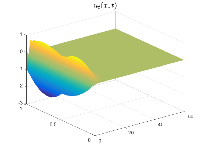
We proceed as follows. In section 2, for system (1) without disturbance, we design a Luenberger state observer and an estimated state based stabilizing control law. We design in section 3 an infinite-dimensional ESO for system (1) to estimated total disturbance and state in real time. An estimated total disturbance and estimated state based stabilizing control law is then designed. Moreover, it is proved that an important couple subsystem including the original equation of the closed-loop is exponential stability and the closed-loop system is bounded. In section 4, some numerical simulations are presented.

We rewrite (1) with $F(t)\equiv 0$ as follows

Our aim in this section is to design a stabilizing control law for system (2) by virtue of only one noncollocated measurement $u_{x}(0,t)$. To this end, we first construct an infinite-dimensional Luenberger state observer as follows

where $\beta,\gamma>0$. Set $\widetilde{u}(x,t)=\widehat{u}(x,t)-u(x,t)$ to get

Denote $\mathbf{H}_{2}=H^{1}(0,1)\times L^{2}(0,1)\times\mathds{C}$, with norm $\|(f,g,\eta)\|^{2}_{\mathbf{H}_{2}}=\int_{0}^{1}|f^{\prime}(x)|^{2}+|g(x)|^{2}+\beta|f(0)|^{2}+|\eta|^{2}/m,$ $(f,g,\eta)\in\mathbf{H}_{2}.$ Then we can write (4) abstractly by

Here $\mathbf{A}_{2}:D(\mathbf{A}_{2})(\subset\mathbf{H}_{2})\rightarrow\mathbf{H}_{2}$ is defined by $\mathbf{A}_{2}(f,$ $g,\eta)=(g,f^{\prime\prime},-f^{\prime}(1)),\;\forall\;(f,g,\eta)\in D(\mathbf{A}_{2})=\{(f,g,$ $\eta)\in\mathbf{H}_{2}|(g,f^{\prime\prime},-f^{\prime}(1))\in\mathbf{H}_{2},f^{\prime}(0)=\gamma g(0)+\beta f(0),$ $\eta=mg(1))\}.$ By [34], $\mathbf{A}_{2}$ generates an exponentially stable $C_{0}$-semigroup, that is, $\|e^{\mathbf{A}_{2}t}\|\leq M_{\mathbf{A}_{2}}e^{\omega_{\mathbf{A}_{2}}t},\;t\geq 0$, where $M_{\mathbf{A}_{2}}$ and $\omega_{\mathbf{A}_{2}}$ are two positive constants. The following Lemma 2 presents that the Riesz basis property of $\mathbf{A}_{2}$ also holds.

Proof. It follows from [34] that operator $(\mathbf{A}_{2},D(\mathbf{A}_{2}))$ generates an exponentially stable $C_{0}$-semigroup, and it is a densely defined and discrete operator on $\mathbf{H}_{2}$. Therefore, for any $\lambda\in\sigma(\mathbf{A}_{2})=\sigma_{P}(\mathbf{A}_{2})$, ${\rm Re}\lambda<0$. We divide the proof into several steps.

Step 1: We claim that for any $\lambda\in\sigma(\mathbf{A}_{2})$, there corresponds one eigenfunction $(f,g,\eta)$ given by

and $\lambda$ satisfies the characteristic equation

This implies that each eigenvalue of $\mathbf{A}_{2}$ is geometrically simple.

Indeed, $f^{\prime\prime}(x)-\lambda^{2}f(x)=0$ implies that $f$ is of the form $f(x)=Ee^{\lambda x}+Fe^{-\lambda x}$. Use the boundary condition $f^{\prime}(0)=(\gamma\lambda+\beta)f(0)$ to derive $E=(1+\gamma)\lambda+\beta,F=(1-\gamma)\lambda-\beta$. We can then derive $\eta=mg(1)=m\lambda f(1)=-\frac{f^{\prime}(1)}{\lambda}$ and (9) by virtue of the boundary condition $f^{\prime}(1)+m\lambda^{2}f(1)=0$.

Step 2: We show that the eigenvalues $\{\lambda_{n}\}_{n=-\infty}^{+\infty}$ have asymptotic expression

where

the corresponding eigenfunction $(f_{n},\lambda_{n}f_{n},$ $m\lambda_{n}f(1))$ of $\mathbf{A}_{2}$ can be chosen such that

where

Now we give the proof. By (9), it follows that

The asymptotic expression (10) is derived directly by Routhe’s theorem. Then we obtain

The combination of (20), (21), (22) and (23) indicates that the asymptotic expression (2) of $F_{n}(x)$ holds.

Step 3: We show that there exist a sequence of generalized eigenfunctions of $\mathbf{A}_{2}$ which forms Riesz basis for $\mathbf{H}_{2}$.

Now we give the proof. Denote

for $\lambda>1$,

for $\lambda<1$. It is easily seen that the operator $\mathbf{T}$ defined by $\mathbf{T}w=P(x)w$ for any $w\in\left(L^{2}(0,1)\right)^{2}$, is a bounded and invertible linear operator on $\left(L^{2}(0,1)\right)^{2}$. Combine this with the fact that $\{(e^{in\pi x},e^{-in\pi x})\}_{n=-\infty}^{+\infty}$ forms Riesz basis for $\left(L^{2}(0,1)\right)^{2}$, to obtain that $\{P(x)(e^{in\pi x},e^{-in\pi x})\}_{n=-\infty}^{+\infty}$ also forms Riesz basis for $\left(L^{2}(0,1)\right)^{2}$. Thereby, $\{(0,0,1,0)\}\bigcup\{(0,0,0,1)\}\bigcup$ $\{(P(x)(e^{in\pi x},e^{-in\pi x}),0,$ $0)$ $\}_{n=-\infty}^{+\infty}$ forms Riesz basis for $\left(L^{2}(0,1)\right)^{2}\times\mathds{C}^{2}$.

From (2), we derive

which implies that, there exists enough big positive integer $N$ such that

Since $\{(0,0,1,0)\}\bigcup\{(0,0,0,1)\}\bigcup\{(P(x)(e^{in\pi x},e^{-in\pi x}),0,0)\}_{n=-\infty}^{+\infty}$ forms Riesz basis for $\big(L^{2}(0,$ $1)\big)^{2}\times\mathds{C}$, it follows by [11, Lemma 1] that there exists a $M\geq N$ such that $\{(0,0,1,0)\}\bigcup\{(0,0,0,1)\}$ $\bigcup\{(P(x)(e^{in\pi x},e^{-in\pi x}),0,0)\}_{n=-M}^{M}\bigcup\{F_{n}\}_{|n|>M}$ forms Riesz basis for $\left(L^{2}(0,1)\right)^{2}\times\mathds{C}^{2}$. We define an isometric isomorphism $\mathbb{T}_{1}:\mathbf{H}_{2}\rightarrow\left(L^{2}(0,1)\right)^{2}\times\mathds{C}^{2}$ by $\mathbb{T}_{1}(f,g,\eta)=(f^{\prime},g,\sqrt{\beta}f(0),\eta),\;\forall\;(f,g,\eta)\in\mathbf{H}_{2}.$ Then there exist $\{W_{n}(x),V_{n}(x),0\}_{n=-M}^{M}\subset\mathbf{H}_{2}$ such that $\{(0,0,1)\}\bigcup\{(W_{n}(x),V_{n}(x),0)\}_{n=-M}^{M}$ $\bigcup\{(\lambda^{-2}_{n}f_{n}(x),\lambda^{-1}_{n}f_{n}(x),-\lambda_{n}^{-3}f^{\prime}_{n}(1))\}_{|n|>M}$ forms Riesz basis for $\mathbf{H}_{2}$. Since $\{(\lambda^{-2}_{n}f_{n}(x),\lambda^{-1}_{n}f_{n}(x),$ $-\lambda_{n}^{-3}f^{\prime}_{n}(1))\}_{n=-\infty}^{\infty}$ is a sequence of generalized eigenvectors of $\mathbf{A}_{2}$, and by [34], $\mathbf{A}_{2}$ is a densely defined and discrete operator, it follows from [11, Theorem 1] that there exists generalized eigenfunctions of $\mathbf{A}_{2}$ that forms Riesz basis for $\mathbf{H}_{2}$. The proof is therefore completed.  

Since the state feedback $U(t)=-\alpha u_{t}-au_{xt}(1,t)$ makes the system (2) exponentially stable [10, 32], Lemma 2 allows us to design the following control law

The closed-loop system is then described by

which is equivalent to

Consider system (2) in Hilbert state space $\mathcal{H}=\mathbf{H}$ $\times\mathbf{H}_{2}$, where $\mathbf{H}=H_{E}^{1}(0,1)\times L^{2}(0,1)\times\mathds{C}$, $H_{E}^{1}(0,1)=\{f$ $\in H^{1}(0,1):f(0)=0\}$. The norm of $\mathbf{H}$ is given by $\|(f,g,\eta)\|^{2}_{\mathbf{H}}=\int_{0}^{1}[|f^{\prime}(x)|^{2}+|g(x)|^{2}]dx+\frac{1}{m+\alpha a}|\eta|^{2},$ $(f,g)\in\mathbf{H}.$ Define the operator $\mathbf{A}:D(\mathbf{A})(\subset\mathbf{H})\rightarrow\mathbf{H}$ by $\mathbf{A}(f,g,\eta)=(g,f^{\prime\prime},-f^{\prime}(1)-\alpha g(1)),\;\forall\;(f,g)\in D(\mathbf{A})=\{(f,g)\in\mathbf{H}|f^{\prime\prime}(1)=0,\eta=mg(1)+af^{\prime}(1)\}.$ By [10, 32], it follows that $\mathbf{A}$ generates an exponentially stable $C_{0}$-semigroup, and there exist a sequence of generalized eigenfunctions of $\mathbf{A}$ that forms Riesz basis for $\mathbf{H}$ provided $\alpha=m/a\neq 1$. In the following Lemma 3, we generalize the result to the case $a\neq m,\alpha>0$.

Proof. We divide the proof into several steps.

Step 1. We claim that operator $(\mathbf{A},D(\mathbf{A}))$ a densely defined and discrete operator on $\mathbf{H}$; for any $\lambda\in\sigma(\mathbf{A})=\sigma_{P}(\mathbf{A})$, ${\rm Re}\lambda<0$.

Indeed, since by [32],$(\mathbf{A},D(\mathbf{A}))$ generates an exponentially stable $C_{0}$-semigroup, it is densely defined and has bounded inverse. Let $(f,g,\eta)\in\mathbf{H}$. Since by Sobolev imbedding theory $H^{2}(0,1)\times H^{1}(0,1)\times\mathds{C}$ is compactly imbedding in $H^{1}(0,1)\times L^{2}(0,1)\times\mathds{C}$, $\mathbf{A}^{-1}$ is compact. Moreover, for any $\lambda\in\sigma(\mathbf{A})=\sigma_{P}(\mathbf{A})$, ${\rm Re}\lambda<0$.

Step 2. We claim that for any $\lambda\in\sigma(\mathbf{A})$, there corresponds one eigenfunction $(f,g,\eta)$ given by

and $\lambda$ satisfies the characteristic equation

This implies that each eigenvalue of $\mathbf{A}$ is geometrically simple.

Step 3: We show that the eigenvalues $\{\lambda_{n}\}_{n=-\infty}^{+\infty}$ have asymptotic expression

References

• [1] J. Auriol, M.D. Meglio, Robust output feedback stabilization for two heterodirectional linear coupled hyperbolic PDEs, Automatica, 115 (2020), 108896.
• [2] R.H. Cannon, E. Schmitz, Initial experiments on the end-point control of a flexible one-link robot, Int. J. Robot. Res., 3 (1984), 62-75.
• [3] G. Chen, A note on the boundary stabilization of the wave equation, SIAM J. Control Optim., 19 (1981), 106-113.
• [4] J. Deutscher, Finite-time output regulation for linear 2×22\times 2 hyperbolic systems using backstepping, Automatica, 75 (2017), 54-62.
• [5] J. Deutscher, J. Gabriel, Periodic output regulation for general linear heterodirectional hyperbolic systems, Automatica, 103 (2019), 208-216.
• [6] J. Deutscher, N. Gehring, Output Feedback Control of Coupled Linear Parabolic ODE-PDE-ODE Systems, IEEE Trans. Automat. Control, DOI 10.1109/TAC.2020.3030763.
• [7] J. Deutscher, J. Gabriel, A backstepping approach to output regulation for coupled linear wave-ODE systems, Automatica, 123 (2020).
• [8] H. Feng, B.Z. Guo, A new active disturbance rejection control to output feedback stabilization for a one-dimensional anti-stable wave equation with disturbance, IEEE Trans. Automat. Control, 62(8) (2017), 3774-3787.
• [9] S.S. Ge, S. Zhang and W. He, Vibration control of an Euler-Bernoulli beam under unknown spatiotemporally varying disturbance, Int. J. Control, 84 (2011), 947-960.
• [10] B.Z. Guo, C.Z. Xu, On the spectrum-determined growth condition of a vibration cable with a tip mass, IEEE Trans. Autom. Control, 45(1) (2000), 89-93.
• [11] B.Z. Guo, R. Yu, The Riesz basis property of discrete operators and application to a Euler-Bernoulli beam equation with boundary linear feedback control, IMA J. Math. Control I., 18(2) (2001), 241-251.
• [12] B.Z. Guo, C.Z. Xu, The stabilization of a one-dimensional wave equation by boundary feedback with non-collocated observation, IEEE Trans. Automat. Control., 52 (2007), 371-377.
• [13] B.Z. Guo, J.M. Wang, K.Y. Yang, Dynamic stabilization of an Euler-Bernoulli beam under boundary control and non-collocated observation, Syst. Control Lett., 57 (2008), 740-749.
• [14] B.Z. Guo, F.F. Jin, Sliding mode and active disturbance rejection control to the stabilization of anti-stable one-dimensional wave equation subject to boundary input disturbance, IEEE Trans. Automat. Control, 58 (2013), 1269-1274.
• [15] B.Z. Guo, F.F. Jin, The active disturbance rejection and sliding mode control approach to the stabilization of Euler-Bernoulli beam equation with boundary input disturbance, Automatica, 49 (2013), 2911-2918.
• [16] B.Z. Guo, J.M. Wang, Control of wave and beam PDEs: the Riesz basis approach, Springer, 2019.
• [17] W. Guo, B.Z. Guo, Adaptive output feedback stabilization for one dimensional wave equation with corrupted observation by harmonic disturbance, SIAM J. Control Optim., 51 (2013), 1679-1706.
• [18] W. He, S.S. Ge, Robust adaptive boundary control of a vibrating string under unknown time-varying disturbance, IEEE Trans. Control Syst. Technol., 20 (2012), 48-58.
• [19] J.Q. Han, From PID to active disturbance rejection control, IEEE Trans. Ind. Electron., 56 (2009), 900-906.
• [20] F.F. Jin, B.Z. Guo, Lyapunov approach to output feedback stabilization for Euler-Bernoulli beam equation with boundary input disturbance, Automatica, 52 (2015), 95-102.
• [21] D. Karagiannis, V. Radisavljevic-Gajic, Sliding mode boundary control for vibration suppression in a pinned-pinned Euler-Bernoulli beam with disturbances, J. Vib. Control, 24(6) (2018), 1109-1122.
• [22] M. Krstic, A. Balogh and A. Smyshlyaev, Backstepping boundary controller and observer for the undamped shear beam, 17th International Symposium on Mathematical Theory of Networks and Systems, 2006.
• [23] M. Krstic, A. Smyshlyaev, Boundary control of PDEs: A course on backstepping designs, Vol. 16. Siam., 2008.
• [24] M. Krstic, B.Z. Guo, A. Balogh and A. Smyshlyaev, Control of a tip-force destabilized shear beam by non-collocated observer-based boundary feedback, SIAM J Control Optim., 47(2008), 553-574.
• [25] M. Krstic, Compensating actuator and sensor dynamics governed by diffusion PDEs, Syst. Control Lett., 58(5) (2009), 372-377.
• [26] M. Krstic and A. Smyshlyaev, Backstepping boundary control for first order hyperbolic PDEs and application to systems with actuator and sensor delays, Syst. Control Lett., 57(2008), 750-758.
• [27] E.B. Lee, Y.C. You, Stabilization of a hybrid (string/point mass) system. In: Proceedings of the 15th International Conference on Systems Engineering. Dayton; 1987. p. 109-112.
• [28] J.J. Liu J, J.M. Wang, Boundary stabilization of a cascade of ODE-wave systems subject to boundary control matched disturbance, Int. J. Robust Nonlinear Control, 27 (2017), 252-280.
• [29] L.Y. Liu, K. Yuan, Noncollocated passivity-based control of a single-link flexible manipulator, Robotica, 21 (2003), 117-135.
• [30] Z.D. Mei, H.C. Zhou, Output Feedback Exponential Stabilization for a One-Dimensional Wave Equation with Control Matched Nonlinear Disturbance, IEEE Trans. Automat. Control, 66(5) (2021), 2273-2280.
• [31] Ö. Morgül,Stabilization and disturbance rejection for the wave equation. In: Proceedings of the 33rd IEEE Conference on Decision and Control (CDC). Orlando; 1994. p. 1776-1777.
• [32] Ö. Morgül, B. Rao, and F. Conrad, On the stabilization of a cable with a tip mass, IEEE Trans. Automat. Control, 39 (1994), 2140-2145.
• [33] Ö. Morgül, Stabilization and disturbance rejection for the beam equation, IEEE Trans. Autom. Control, 46 (2001), 1913-1918.
• [34] B.P. Rao, Decay estimates of solutions for a hybrid system of flexible structures, Euro. J. Appl. Math., 4 (1993), 303-319.
• [35] P. Rideau, Contrôle d’un assemblage de poutres flexibles par des capteurs-actionneurs ponctuels: Étude du spectre du système, Thèse de l’École Nationale Supérieure des Mines de Paris. Sophia-Antipolis, France, Nov. 1985.
• [36] L.L. Su, J.M. Wang, Stabilisation of an anti-stable joint string with boundary disturbance, Int. J. Control, 93(5) (2020), 1027-1038.
• [37] A.Smyshlyaev, M. Krstic, Backstepping observers for a class of parabolic PDEs, Syst. Control Lett., 54 (2005), 613-625.
• [38] Z.Q. Tian, H. Feng, Stabilization of one-dimensional wave equation by non-collocated boundary feedback, Eur. J. Control, 32 (2016), 39-42.
• [39] J. Wang, S.X. Tang, M. Krstic, Adaptive output-feedback control of torsional vibration in off-shore rotary oil drilling systems, Automatica, 111 (2020), 108640.
• [40] Y.R. Xie, G.Q. Xu, Stabilization of a wave equation with a tip mass based on disturbance observer of time-varying gain, J. Dyn. Control. Syst., 23 (2017):667-677
• [41] H.C. Zhou, B.Z. Guo, Unknown input observer design and output feedback stabilization for multi-dimensional wave equation with boundary control matched uncertainty, J. Differ. Equations, 263 (2017), 2213-2246.
• [42] H.C. Zhou, H. Feng, Disturbance estimator based output feedback exponential stabilization for Euler-Bernoulli beam equation with boundary control, Automatica, 91 (2018), 79-88.
• [43] H.C. Zhou, G. Weiss, Output feedback exponential stabilization for one-dimensional unstable wave equations with boundary control matched disturbance, SIAM J. Control Optim., 56 (2018), 4098-4129.
• [44] H.C. Zhou and H. Feng, Stabilization for Euler-Bernoulli beam equation with boundary moment control and disturbance via a new disturbance estimator, J. Dyn. Control. Syst., 27 (2021), 247-259.