∎
Omni: Automated Ensemble with Unexpected Models against Adversarial Evasion Attack
Abstract
Background: Machine learning-based security detection models have become prevalent in modern malware and intrusion detection systems. However, previous studies show that such models are susceptible to adversarial evasion attacks. In this type of attack, inputs (i.e., adversarial examples) are specially crafted by intelligent malicious adversaries, with the aim of being misclassified by existing state-of-the-art models (e.g., deep neural networks). Once the attackers can fool a classifier to think that a malicious input is actually benign, they can render a machine learning-based malware or intrusion detection system ineffective.
Goal: To help security practitioners and researchers build a more robust model against non-adaptive, white-box and non-targeted adversarial evasion attacks through the idea of ensemble model.
Method: We propose an approach called Omni, the main idea of which is to explore methods that create an ensemble of “unexpected models”; i.e., models whose control hyperparameters have a large distance to the hyperparameters of an adversary’s target model, with which we then make an optimized weighted ensemble prediction.
Result: In studies with five types of adversarial evasion attacks (FGSM, BIM, JSMA, DeepFool and Carlini-Wagner) on five security datasets (NSL-KDD, CIC-IDS-2017, CSE-CIC-IDS2018, CICAndMal2017 and the Contagio PDF dataset), we show Omni is a promising approach as a defense strategy against adversarial attacks when compared with other baseline treatments.
Conclusion: When employing ensemble defense against adversarial evasion attacks, we suggest to create ensemble with unexpected models that are distant from the attacker’s expected model (i.e., target model) through methods such as hyperparameter optimization.
Declarations:
Funding: This work was partially funded by NSF grant #1909516.
Conflicts of interest/Competing interests: The authors have no relevant financial or non-financial interests to disclose.
Keywords:
Hyperparameter Optimization Ensemble Defense Adversarial Evasion Attack1 Introduction
With the growing reliance on information technology, cybercrime is a serious threat to the economy, military and other industrial sectors Bissell et al. 2019; Jang-Jaccard and Nepal 2014; Chang et al. 2019; Opderbeck 2015; Roškot et al. 2020. In 2019, the damage cost caused by malware and cybercrime exceeded a trillion dollars Morgan 2019. For example, a March 2019 ransomware attack on aluminum producer Norsk Hydro caused 60 million pounds of remediation cost Sechel 2019. The attack brought production to a halt at 170 sites around the world. More generally, a 2019 study by Accenture reports that cybercrime will cost US $5.2 trillion over the next five years Bissell et al. 2019 Alarming, that cost is growing. That same report documents that in the United States, the annual average cost to organization of malicious software has grown 29% in the last year.
To counter those threats, machine learning algorithms are being widely applied to security critical tasks, such as malware detection and intrusion detection. For example, security practitioners and researchers build detection models that utilize learned patterns to detect whether a new file (e.g., PDF file) or an application (e.g., Android app) or a network traffic becomes a security threat Maiorca et al. 2013; Smutz and Stavrou 2012; Bhat and Dutta 2019; Arp et al. 2014. But paradoxically, machine learning also introduces a new attack vector for motivated adversariesBarreno et al. 2006; Biggio and Roli 2018. An active research field called adversarial machine learning has received a significant amount of attention over the last decade. Adversarial machine learning is a technique that attempts to fool or misguide a machine learning-based model with malicious inputs. This technique was first studied in spam filtering Dalvi et al. 2004; Lowd and Meek 2005a; Lowd and Meek 2005b and later on since 2014, Szegedy et al. Szegedy et al. 2013 found that small perturbations in images can cause misclassification in neural network classifiers which attracted more studies in domains such as computer vision. While at the same time, this technique is also widely studied in the security domain. Adversarial evasion attack Biggio et al. 2013a is one of the most prevalent types of adversarial machine learning attacks that happens during the testing stage in the machine learning pipeline. In this attack, attackers try to evade the detection system by manipulating the testing data, resulting in a wrong model classification. The core of adversarial evasion attack is that when an attacker can fool a classifier to think that a malicious input (e.g., malicious Android application or network traffic) is actually benign, they can render a machine learning-based malware detector or intrusion detector ineffective.
Prior studies have tried Tramèr et al. 2018; Smutz and Stavrou 2016; Kantchelian et al. 2016 to thwart evasion attacks by building a more robust and complex model via ensemble learning Dietterich et al. 2002. Ensemble learning is the process of (a) building multiple models and then (b) polling across the models to arrive at a final decision. In theory, ensemble learning tends to defend against adversarial evasion attack because attackers have to craft payloads (i.e., adversarial examples) that are able to subvert all constituent models at once, which makes it more difficult to be successful. However, some other studies Zhang et al. 2020; Zhang et al. 2018; He et al. 2017; Tramèr et al. 2018; Papernot et al. 2016e caution that adversaries can still defeat ensemble-based strategy. For example, Papernot et al. Papernot et al. 2016e find that, even when ensemble classifiers are used, adversarial attackers can still manage to use their own models to find ways to “transfer” the adversarial examples to a victim model (i.e., attacker’s target model), even if (a) the adversary has little knowledge of the victim model; and even if (b) the defender uses an ensemble of classifiers.
The starting point for our research in this paper is the following observation. Prior work on ensemble learning against adversarial evasion attack Tramèr et al. 2018; Smutz and Stavrou 2016; Kantchelian et al. 2016 barely explored the range of options available within a model or explored few different models. For example, some researchers build their ensemble-based approaches using a small number of constitute models; e.g., Kantchelian et al. Kantchelian et al. 2016 use seven constitute models in their ensemble classifier. Such kind of small size ensemble classifier usually does not yield the optimal prediction performance Hernández-Lobato et al. 2013. However, as shown in Table 1, malware or intrusion detection models can be built from a space of trillions of options (i.e., hyperparameter choices of a model). The small space of ensembles used in previous work barely scratches the surface of the large space of options within ensemble generation.
| Hyperparameter | Ranges | ||||
|---|---|---|---|---|---|
|
| ||||
|
| ||||
| First layer dense | quniform(30, 150, 1) | ||||
| Second layer dense | quniform(30, 50, 1) | ||||
| Third layer dense | quniform(10, 32, 1) | ||||
| Drop out rate | uniform(0.0, 0.5) | ||||
| Optimizer |
| ||||
| Batch size | 16, 32, 64, 128 | ||||
| Number of epochs | quniform(5, 20, 1) | ||||
| Learning rate | 0.001, 0.01, 0.1 |
- •
* Note: quniform(, , ) is a function returns a value like , while uniform(, ) returns a value uniformly between and .
Accordingly, the core innovation of this paper is the proposed approach called Omni. This method uses hyperparameter optimization Feurer and Hutter 2019 algorithms that build an ensemble system by exploring trillion of model options. Such optimization algorithms seek the set of hyperparameters of a given machine learning algorithm which return the optimal evaluation performance. In a machine learning algorithm, hyperparameters are properties that control the behaviors of the machine learning algorithms. For example, when reasoning about “-nearest neighbors”, the hyperparameter “” decides how many neighbors to use for making a decision.
While exploring a large number of models (such as the trillions of options from Table 1), our Omni method learns the “expected model”; i.e. the optimal model from hyperparameter optimization, which is used in normal prediction. This model is the target of attackers and hence then becomes the victim model. Next, Omni’s optimizer surveys the hyperparameter space of models to find “unexpected models”; i.e. models that are (a) performing well (i.e., sub-optimal models) and (b) dissimilar to the expected model (i.e., in the architecture). More specifically:
- •
For hyperparameter optimization, we search a large space of possible configurations of a model to initialize a large model pool.
- •
The expected model is a model from the model pool that performs best (under no attack). We call this model “expected” since we conjecture that this model would be the target of an attacker, and becomes a victim model.
- •
We introduce an idea called model distance, which is a numeric value indicating the degree of similarity of two models’ hyperparameter configurations. A large model distance value means that two models are more likely to be different in their model architecture.
- •
The unexpected models are those whose performance within some small of the expected model but are more than some distance away from the expected model.
- •
Those unexpected models are combined into a weighted ensemble, in which each model in the ensemble with a weight . The final prediction of this ensemble is the combined prediction of each model times its weight . These weights are further optimized by an evolutionary algorithm that finds optimal setting that maximizes prediction performance.
- •
The final weighted ensemble, with its optimized weight setting is then deployed against evasion attacks.
The rest of the paper shows empirically that the results of using Omni as a defense method against adversarial evasion attacks is promising. Background and related work is discussed in Section 2. We introduce threat model, adversarial evasion attack strategies as well as the proposed approach in Section 3. We then describe our datasets and experiment rigs in Section 4. For this studies, we use:
- •
Five sophisticated adversarial evasion attack strategies; i.e. FGSM Goodfellow et al. 2015, BIM Kurakin et al. 2017, JSMA Papernot et al. 2016c, DeepFool Moosavi-Dezfooli et al. 2016 and Carlini-Wagner Carlini and Wagner 2017a; Carlini and Wagner 2017b;
- •
And five security datasets; i.e. NSL-KDD Canadian Institute for Cybersecurity 2009, CIC-IDS-2017 Sharafaldin et al. 2018, CSE-CIC-IDS2018 Sharafaldin et al. 2018, CICAndMal2017 Lashkari et al. 2018 and the Contagio PDF dataset Contagio 2020.
As shown in Section 5 (i.e., the results section), Omni demonstrates its advantages when compared with other baseline treatments such as adversarial training, random ensemble and average weight ensemble. We discuss more about the nature of Omni and other issues in Section 6 and threats to validity in Section 7 then present the conclusion and future directions to extend this work in Section 8. Here we conclude:
A well-designed weighted ensemble system is a promising approach to defend against adversarial evasion attack.
and
When using ensemble learning as a defense method against adversarial evasion attacks, we suggest to create ensemble with unexpected models that are distant from the attacker’s expected model (i.e., target model) through methods such as hyperparameter optimization.
2 Background and Related Works
2.1 Machine Learning for Security & Adversarial Machine Learning
The global security threat continues to evolve at a rapid pace, with a rising number of types of threats. For example, previous studies have shown many kinds of malicious software:
- •
Malware that is a malicious file or hidden within files; e.g. PDF files can carry malicious code Smith 2001.
- •
Ransomware that encrypts a victim’s files then demands a ransom from the victims to restore access to the data upon payment. For example, a March 2019 ransomware attack on aluminum producer Norsk Hydro caused 60 million pounds of remediation cost. The attack brought production to a halt at 170 sites around the world (some 22,000 computers were affected across 40 different networks) Sechel 2019.
- •
Industrial espionage software that infects, then destroyed industrial machinery; e.g. the Stuxnet virus used to damage centrifuges at Iran’s Natanz uranium enrichment facility Langner 2011.
- •
In the social network realm, Facebook estimated that hackers stole user information from nearly 30 million people through malicious software Queenie Wong 2018.
- •
According to the International Data Corporation (IDC), the Android operating system covers around 85% of the world’s smartphone market. Because of its increasing popularity, Android is drawing the attention of malware developers and cyber-attackers. Android malware families that are popular are spyware, bots, Adware, Potentially Unwanted Applications (PUA), Trojans, and Trojan spyware, which affect millions of Android users Bhat and Dutta 2019.
- •
Other kinds of malicious software Monshizadeh and Yan 2014 include (a) scareware that socially engineers anxiety, or the perception of a threat, to manipulate users into e.g. buying unwanted software; (b) adware that throws advertisements up on your screen (most often within a web browser); and (c) software that infects your computer then, without your permission of knowledge, mounts a denial of service attack on other computers.
Security practitioners now routinely add security detectors to their environments, which are machine learning models that utilize known detective patterns to verify whether an application becomes a threat. Such detectors can be built in many ways including (but not restricted to) building a classifier to examine a web page for malicious content Canali et al. 2011; Eshete et al. 2012; constructing multiple classifier systems to classify spam emails Biggio et al. 2010; building classifiers to detect malicious PDF files Xu et al. 2016; applying machine learning to detect Android malware Grosse et al. 2017b; designing supervised learning algorithm to classify HTTP logs Liu et al. 2017; designing machine learning models to detect ransomware Muñoz-González et al. 2017; and detecting malicious PowerShell commands using deep neural networks Hendler et al. 2018.
Previous research works on adversarial machine learning are mainly focused on computer vision which solves tasks such as image recognition Goodfellow et al. 2015; Papernot et al. 2017b. However, adversarial machine learning can also be applied to other domains, such as the security domain, since most of them are not data dependent attacks. Adversarial machine learning studies in the security domain (e.g., intrusion detection) received more and more attention in recent years. To understand the current thinking of adversarial machine learning in the security domain, we conduct a literature review of papers during the last decade. We use google scholar to trace publications and their citations and search papers that fall into this topic.
Table 2 lists relevant work from the last decade. We observe that researchers are more interested in attacks than defense, while at the same time, malware detection and intrusion detection receive more attention than other tasks (e.g., spam filtering), which also motivate our study.
| Ref | Year | Citation | Tasks | Attack/Defense |
|---|---|---|---|---|
| Biggio et al. 2010 | 2010 | 175 | Spam Filtering | ◑ |
| Zhou et al. 2012 | 2012 | 87 | Spam Filtering | ◐ |
| Smutz and Stavrou 2012 | 2012 | 207 | Malicious PDF | ◐ |
| Biggio et al. 2013b | 2013 | 91 | Program Malware Detection | ◐ |
| Biggio et al. 2013a | 2013 | 471 | Malicious PDF Detection | ◐ |
| Maiorca et al. 2013 | 2013 | 101 | Malicious PDF Detection | ◐ |
| Laskov et al. 2014 | 2014 | 239 | Malicious PDF Detection | ● |
| Biggio et al. 2014 | 2014 | 80 | Spam and Malware Detection | ◐ |
| Biggio et al. 2014 | 2014 | 95 | Program Malware Detection | ◐ |
| Zhang et al. 2015 | 2015 | 126 | Spam Filtering and Malicious PDF Detection | ◑ |
| Xiao et al. 2015 | 2015 | 211 | Malicious PDF Detection | ◑ |
| Xiao et al. 2015 | 2015 | 160 | Malicious PDF Detection | ◐ |
| Grosse et al. 2016 | 2016 | 229 | Android Malware Detection | ◐ |
| Tramèr et al. 2016 | 2016 | 623 | Spam Filtering | ◐ |
| Xu et al. 2016 | 2016 | 243 | Malicious PDF Detection | ◐ |
| Grosse et al. 2017a | 2017 | 255 | Android Malware Detection | ◐ |
| Strauss et al. 2017 | 2017 | 57 | Android Malware Detection | ● |
| Hu and Tan 2017 | 2017 | 172 | Program Malware Detection | ◐ |
| Dang et al. 2017 | 2017 | 50 | Malicious PDF Detection | ◐ |
| Chen et al. 2018 | 2018 | 77 | Android Malware Detection | ◐ |
| Demontis et al. 2019 | 2019 | 20 | Android Malware Detection | ◐ |
2.2 Adversarial Defense Strategy
Researchers have proposed various solutions against adversarial machine learning attacks. One way to categorize defense strategies is based on different phases in the machine learning pipeline. Another way is to divide into two types, i.e., reactive defenses and proactive defenses. The former focuses on detecting adversarial examples separately from a trained classifier, while the latter focuses on building classifiers that are robust to adversarial examples. In the following section, we provide a summary of existing defense methods especially against adversarial evasion attacks.
Defense during the testing phases includes adversarial training, gradient masking, defensive distillation, and ensemble learning. The idea of adversarial training Tramèr et al. 2018; Na et al. 2018; Madry et al. 2018; Farnia et al. 2019; Shafahi et al. 2019; Yin et al. 2019 is to build a “golden” dataset that ideally contains a set of curated attacks and normal data that are representative of the target system. The data is then used when training the model. Intuitively, if the model sees adversarial examples during training, its performance during prediction will be improved for adversarial examples generated in the same way. However, the problem with adversarial training is that it suffers from an optimized attack or adaptive attack, since this method only defends the model against the same attacks used to craft the examples originally included during training.
Gradient masking Papernot et al. 2018 is a technique that hides the model gradients to reduce model’s sensitivity to adversarial examples. However, later work Athalye et al. 2018 shows that the gradient masking tactic does not work because of the transferability property of adversarial examples. The attackers can still build a substitute model and transfer the attacks.
Defensive distillation Papernot et al. 2016d tries to generate a new model whose gradients are much smaller than the original undefended model. If gradients are very small, some gradient-based attacks are no longer useful, as the attacker would need great distortions of the input data to achieve a sufficient change in the loss function. However, this method was quickly proved to be ineffective Carlini and Wagner 2016. With a slight modification to a standard attack, attackers can still find adversarial examples on distilled networks.
Ensemble learning Dietterich et al. 2002 is another widely used defense mechanism, in which multiple classifiers are combined together to improve classifier robustness. For example, Biggio et. al. Biggio et al. 2010 investigated ways to build a multiple classifier system (MCS) that improved the robustness of linear classifiers. They argued that randomization-based MCS construction techniques, such as bagging and random subspace method (RSM), were effective in improving classification accuracy. Tramer et. al. Tramèr et al. 2018 introduced a technique called ensemble adversarial training that augments training data with perturbations transferred from other models to increase robustness. Kariyappa et. al. Kariyappa and Qureshi 2019 showed that an ensemble of models with misaligned loss gradients can provide an effective defense against transfer-based attacks. Besides, some other studies Tramèr et al. 2018; Smutz and Stavrou 2016; Kantchelian et al. 2016 also show ways to respond to adversarial evasion attack via ensemble learning.
However, some other prior results are not supportive of the use of ensemble learning for defense purposes Zhang et al. 2020; Zhang et al. 2018; He et al. 2017; Tramèr et al. 2018; Papernot et al. 2016e. For example, Zhang et al. Zhang et al. 2020 show that a discrete-valued tree ensemble classifier can be easily evaded by adversarial inputs manipulated based only on the model decision outputs. Zhang et al. Zhang et al. 2018 investigate the evasion attacks in a more practical setting where attackers do not know the details of classifier, but instead they may acquire only a portion of the labeled data or a replacement dataset for learning the target decision boundary. They argue that ensemble classifiers are not necessarily more robust under a least effort attack based on gradient descent. He et al He et al. 2017 demonstrate that an adaptive adversary can create adversarial examples successfully with low distortion, hence implies that ensemble of weak defenses is not sufficient to provide strong defense against adversarial examples. Papernot et al. Papernot et al. 2016e find the transferability property of adversarial examples also make ensemble classifier less effective.
As mentioned in the introduction section, we argue that there is an issue with prior research using ensemble methods for defense purpose. Specifically, the exploration space for their ensemble systems was too small, while our reading of Table 1 indicates that there are trillions of options to configure a security detection model (the building block of the ensemble system). The rest of this paper proposes a novel method that takes better advantage of that large space of options.
2.3 Hyperparameter Optimization
Given a space of hyperparameter options like Table 1, hyperparameter optimization can be represented as follows:
| (1) |
Here represents the objective to be maximize, e.g. recall or accuracy. is the set of hyperparameters that produce the best score, while can be any value from domain .
Existing hyperparameter optimization algorithms can mainly fall into three categories:
- •
Exhaustive search of hyperparameter space;
- •
Using evolutionary algorithm;
- •
Utilizing Bayesian optimization.
The first category includes manual search, grid search and random search. The search space of each hyperparameter is discretized, and the total search space is discretized as the Cartesian products of them. When using manual search, we choose some model hyperparameters based on our own experience. We then train the model, evaluate its performance and start the process again. This loop is repeated until a satisfactory score is found. The grid search Bergstra et al. 2011 algorithm would traverse all the configurations and select the best one, which is computationally costly and can easily suffer from the “curse of dimensionality”. As a variation of grid search algorithm, random search algorithm Bergstra and Bengio 2012 randomly samples the configurations to reach a predefined fixed sampling density. With purely random sampling, the selected hyperparameters give a non-uniform sampling density of the search space.
As for the second category, the evolutionary algorithm in hyperparameter optimization Young et al. 2015 takes its inspiration from the process of natural selection. This algorithm allows a selective exploration of the operation range using fitness function that determines which is going to be the next point to be sampled.
Both of them are good options for simple optimization problems due to easy implementation of algorithms. However, for complex objective functions, both methods are relatively inefficient because there is no guarantee that they can find an optimal solution except if the configuration space is thoroughly searched. This is a problem if the evaluations of the objective function are not cheap, i.e., the models take a significant amount of time to run with lots of computational resources, and they are uninformed of the information gained from previous evaluations. For example, they do not choose the next hyperparameter based on previous results, which leads to wasting a large amount of time evaluating “bad” hyperparameters instead of focusing on the most promising hyperparameters.
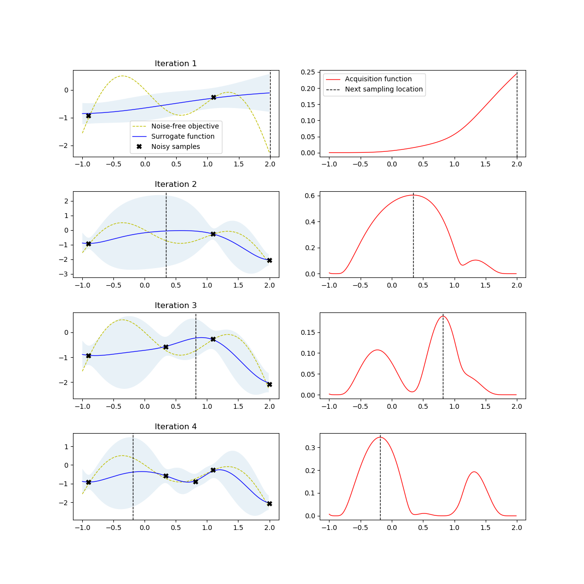
Bayesian optimization Snoek et al. 2012; Shahriari et al. 2015 address such concerns by keeping track of past evaluation results. The principle of Bayesian optimization is using those results to build a probability model of objective function, and map hyperparameters to a probability of a score on the objective function, and therefore use it to select the most promising hyperparameters to evaluate in the true objective function. This method is also called Sequential Model-Based Optimization (SMBO). Figure 1 shows an example process of Bayesian optimization.
The probability representation of the objective function is called surrogate function or response surface because it is a high-dimensional mapping of hyperparameters to the probability of a score on the objective function. The surrogate function is much easier to optimize than the objective function and Bayesian methods work by finding the next set of hyperparameters to evaluate the actual objective function by selecting hyperparameters that perform best on the surrogate function. This method continually updates the surrogate probability model after each evaluation of the objective function.
Variations of SMBO methods differ in how to build a surrogate of the objective function and the criterion used to select the next hyperparameters. Several choices for surrogates function are Gaussian Processes, Random Forest Regression, and Tree Parzen Estimators (TPE) Bergstra et al. 2011, and one of the most common choices for acquisition function is Expected Improvement Snoek et al. 2012. Specifically, our method chooses TPE as the surrogate function and Expected Improvement as the acquisition function, which is popular to use. TPE handles hyperparameter space in a tree-structured fashion, and during iterations, TPE divides observations into two groups. One group only contains observations that give the best scores after evaluation and the other group contains all the rest. The fraction of the best observation is usually defined as 10% to 25% of observations. TPE then models the likelihood probability of each group, and using the likelihood probability from the first group, TPE sampled a bunch of candidates, from which we seek a candidate that is more likely to be in the first group and less likely to be in the second group. TPE also uses the parzen-window density estimators, with which each sample defines Gaussian distribution with specified mean (i.e., the value of the hyperparameter) and standard deviation. These points then stack together and normalized to assure that output is Probability Density Function (PDF). For Expected Improvement, finding the values that will yield the greatest expected improvement in the surrogate function is much cheaper than evaluating the objective function itself.
3 Methodology
In this section, we first introduce some guidelines that help direct our work. We then discuss the adversarial threat model. Next, we introduce the methods of generating adversarial examples for evasion attack. We then demonstrate the details of our ensemble learning based approach Omni.
3.1 Some Guidelines
Before we go deeper into our proposed method, we first introduce several general design principles that are not specific to any individual research question. Carlini et al. Carlini et al. 2019 provide practical advices for evaluating adversarial defense that is intended to be robust to adversarial examples. Specifically, their work shows a list of principles of rigorous evaluations and a checklist of recommendations. Motivated by their work, here we list some example principles that are applicable to our work. Besides, we also add some other principles that beyond Carlini et al.’s recommendations.
- •
P1: State a precise threat model that defense is supposed to be effective under.
- –
Our threat model is described in Section 3.2.
- –
- •
P2: Release models and source code.
- •
P3: Report clean model accuracy when not under attack.
- –
In the results section, we take care to present our pre-attack accuracy as well as other results.
- –
- •
P4: Describe the attacks applied, and report all attack hyperparameters.
- •
P5: Apply a diverse set of attacks.
- •
P6: Report per-case attack success rate.
- •
P7: Record the runtime of hyperparameter tuning phase.
- •
P8: Any work with a stochastic component need to repeat experiments multiple times. As shown below, all our results come from multiple 80% train, 20% test runs where, for each run, the random number seed was changed.
3.2 Threat Model
The machine learning adversarial threat model is a structured framework that lays out all the possible threat vectors on the machine learning system. We provide here a detailed threat model for evasion attacks against deep neural networks. This threat model consists of defining the adversary’s goals, knowledge of the target system, and capabilities of manipulating the testing data.
Adversary’s goals. The goal of the adversary attackers is to impact target model’s prediction performance by causing its misclassification in the testing phase, thus malicious payload can avoid being detected. For example, in a security system (e.g., intrusion detection or malware detection), the attackers want a specific class (e.g., “malicious”) to be classified as a specific other class (e.g., “benign”).
Adversary’s knowledge. The smart adversary attackers are essentially assumed to obtain the internal knowledge of the target model through other approaches. For example, we assume that attackers are able to collect information, including but not limited to model architecture, number of layers, optimization algorithm used, gradients of loss function, testing data, and therefore could successfully carry out white-box attacks Goodfellow et al. 2015 to the target model. Prior study Carlini and Wagner 2017b has shown that accessing model’s gradients is one of the most efficient ways to fool the target models with crafted adversarial examples. When a defense system is applied, the attackers are also assumed to obtain its knowledge and thus challenge the defense system.
Adversary’s capability. In adversarial evasion attacks, the adversary attackers are assumed to be able to perturb the testing dataset. In addition, the adversary attackers are also able to acquire prediction results from the target model. We assume adversarial attacks are carried out at the inference time (i.e., testing time), which means the attackers are only able to perturb the immediate inputs, while not be able to manipulate the training dataset.
Furthermore, we make some justifications about the threat model. Firstly, we limit the scope of study that the attackers will try to evade a single model with crafted adversarial examples. Attacking multiple models with adversarial examples Kwon et al. 2018 is another interesting research direction which we would like to explore in future work. In such type of attack, attackers generate multi-targeted adversarial examples which can be found useful for them to make multiple models to recognize a single data (e.g., image) as different classes.
Secondly, there is a growing interest in different types of privacy-related attacks (e.g., model extraction attack Papernot et al. 2017a) which make the leakage of model information possible Rigaki and Garcia 2020. For example, in an example from the previous study Juuti et al. 2019, some business models are hosted in a secure cloud that allow user clients to query the models via cloud-based prediction APIs. These prediction APIs are suffered from being exploited with model extraction attacks. The target model can be used as an oracle for returning predictions for the samples that attackers submit. Such kind of attempts can further be iteratively executed for attackers to maximize the information extraction about model internals.
Thirdly, our threat model also does not assume adaptive adversarial attacks which are more novel and specifically designed to target a given defense mechanism. In addition, the white-box adversarial attacks in this threat model are non-targeted attacks. Specifically, the aim of non-targeted attacks is to cause samples to be classified incorrectly while targeted attacks would cause samples to be misclassified as specific target class.
3.3 Adversarial Attack Strategy
Adversarial examples Szegedy et al. 2014 or adversarial inputs are examples that are intentionally crafted by attackers by making small perturbations to the input data to cause a machine learning model to produce an incorrect output. Machine learning models, including existing state-of-the-art models such as neural networks lack the ability to classify adversarial examples correctly. A very active research field relevant to this topic is how to craft adversarial examples to fool models. We choose five methods that are widely studied in this domain.
Fast Gradient Sign Method (FGSM) Goodfellow et al. 2015 is a method to generate adversarial examples using model’s gradient information. Each data in the clean dataset is modified by adding or subtracting an almost imperceptible error of . If the sign of the gradient is positive, will be added, and vice versa. Equation 2 formalizes the way to generate adversarial examples by FGSM. In this expression, we note that is the adversarial dataset, is the original input dataset, is the original output label, is the multiplier to ensure the small perturbation, is the model hyperparameters, is the gradient, and is the loss function.
| (2) |
Under this assumption, the gradient of the loss function indicates the direction in which we need to change the input vector to produce a maximal change in the loss. In order to keep the size of the perturbation small, we only extract the sign of the gradient, not its actual norm, and scale it by a small factor epsilon.
Basic Iterative Method (BIM) Kurakin et al. 2017 is an iterative version of FGSM where a small perturbation is added in each iteration. There are two versions of BIM attack: BIM-A and BIM-B. The BIM-A method stops the iteration as soon as mislcassification is achieved. In the BIM-B method, iterations only stop after a fixed number of rounds.
Jacobian-based Saliency Map (JSMA) Papernot et al. 2016c is an iterative method that achieves misclassification of input to any pre-specified class. It uses feature selection with the aim of minimizing the number of features perturbed (i.e., the distance metric).
This method includes the computation of saliency maps for an input sample, which contain the saliency values for each input feature. These values indicate how much the modification of that feature will perturb the classification process, how much different from each target class. Features are then selected in decreasing order of saliency value, and the feature with the max value in this map is perturbed by . The saliency map is created in the following way:
| (3) |
We modify JSMA, so as to flip the feature values from 0 to 1, or 1 to 0 in the perturb step.
DeepFool Moosavi-Dezfooli et al. 2016 works in an iterative manner, with the aim of minimizing the euclidean distance between perturbed samples and original samples (i.e., the distance metric). Specifically, the generation of adversarial samples consists of the analytical calculation of a linear approximation of the decision boundary that separates sample from different classes, and then adding a perturbation perpendicular to that decision boundary, which brings the input closest to a linear approximation of the decision boundary. The algorithm terminates once misclassification is achieved.
Carlini-Wagner (C & W) attack Carlini and Wagner 2017a; Carlini and Wagner 2017b builds an optimization-based attack where the goal is to find the smallest perturbation that can cause a misclassification. If we consider input and noise , this attack finds the adversarial instance by finding the smallest noise added to the input that will change the classification to a class . The noise level is measured in terms of distance. Finding the minimum distance of while ensuring that the output will have a class is not a trivial optimization problem. Instead, Carlini-Wagner attack solves the optimization problem of the form:
| (4) |
where ; is an objective function that drives the input to be misclassified; and is a suitably chosen constant.
3.4 Omni: Building Ensembles of “Unexpected” Models
3.4.1 System Architecture

The basic idea of Omni is to build a more robust ensemble classifier against adversarial attacks that aim at a target model. In order to create such robust ensemble classifier, we employ several novel tricks. The architecture of Omni is presented in Figure 2. In our method, we first apply a hyperparameter tuning method named Bayesian optimization to train a set of models that build a model pool. We ranked the models in the model pool by prediction performance, and pick the model with optimal performance for normal prediction. This model is thus becoming the target model of the adversarial attackers.
As the defense strategy against the adversarial attacks, the ensemble classifier (i.e., Omni) selects other candidate models from the model pool rather than the target model. Those candidate models are able to achieve sub-optimal prediction performance as well as with a distance (in terms of hyperparameter) to the target model. Those picked models are further optimized with weights in the ensemble classifier in order to perform better (i.e., robust) against adversarial attacks.
Besides, we assume that users are more likely to train their models and further optimize their models towards the goal of better prediction performance. We start with such point and choose the optimal model as the attacker’s target since a sub-optimal model might suffer from misclassification even under normal prediction.
3.4.2 Build Ensemble Classifier
Since Omni is an ensemble learning based approach, we then come up with two questions: 1) How to select models for the ensemble system? and 2) How to aggregate those models across the ensemble system?
Unexpected model selection. In our method, we first run our optimizer in the usual manner to find parameters resulting in the model with the highest accuracy. We call this model the expected model since this is the model we would expect the attackers to learn.
Note that, as a side effect of this process, we have a large pool of models; i.e. all the other models explored by the optimizer before arriving at the best one. In this pool, we then hunt for “useful” unexpected models; i.e. models whose hyperparameters are distant from the expected models. Here, by “useful” we mean the models that are performing nearly as well as the expected model. Using ensemble learning, we then create a combined classifier from the unexpected models.
Why do we use those“unexpected models”? Previous work Papernot et al. 2016b; Demontis et al. 2019 show that adversarial evasion attack has the ability to transfer from one model to another model. That is, specially crafted adversarial examples that cause misprediction of model are also likely to mislead a different model . However, this transferability becomes less reliable when two models have different structures Papernot et al. 2016b. For example:
- •
For cross-technique models (e.g., SVM and DNN), attacks from SVM to DNN are less effective than from SVM to SVM.
- •
For intra-technique models (e.g., both models are DNN), attacks from DNN to DNN are also less effective than from DNN to itself.
- •
Generalizing these examples, the rest of this paper tests that we can generate different structures (that makes an adversary harder to figure out defender’s decision boundary), just be picking models that are some distance “” from the expected model (measured using the distance between the hyperparameters.
To implement the above, we need some measure of “distance” , that denotes an “unexpected model”. To compute that, we note that the hyperparameters in Table 1 are in various forms, which involve both discrete categorical and continuous numerical values. Traditional metrics such as Euclidean distance or cosine distance cannot calculate distance between two entities whose attributes have a mix of values. Gower distance Gower 1971 is a distance measure that can be used to address this concern. This measure is defined as follows:
| (5) |
where is the weight of variable between observation and and is the distance between and on variable . Moreover, applies different formulas to categorical and numerical variables. Specifically, for categorical variable, if two observations are the same then the distance of them is assigned , otherwise assigned . For numerical variable, the absolute difference is calculated between observation and , then the result is scaled to range by dividing the range of values of variable . The following equations describe how to calculate categorical and numerical variables respectively, where is the value of variable for observation .
| (6) |
| (7) |
The Gower distance allows to assign a weight to each individual variable base on the importance of that variable in the distance calculation. For simplicity, we use the equal weight in our study.
Unexpected model aggregation. There are various ways of combining unexpected models, in our work, Omni uses a bagging approach named weighted ensemble. When optimizing these weights, we seek to maximize the accuracy of the ensemble.
The way of searching for the weight values is an optimization process. We propose to use an evolutionary algorithm named differential evolution (DE), shown in Figure 3, to solve the function optimization. This optimizer is inspired by biology natural selection process and follows the rule of Darwin’s “survival of the fitness” evolution theory. The general idea of this algorithm is to randomly select some samples from a population. The selected samples are then combined with a scheme to generate a new sample. If the new sample is better after evaluation with target function, then the previous samples are replaced. After several iterations, the population will converge towards the optimal solution. Differential evolution algorithm has very few parameters to adjust, so it is easy to implement and convenient to use.
The premise of the Figure 3 code is that the best way to mutate the existing optimizations is to extrapolate between current solutions (stored in the frontier list). Three solutions are selected at random from the frontier. For each tuning parameter , at some probability , DE replaces the old solution with new where and is a parameter controlling differential weight.
The main loop of DE runs over the frontier of size , replacing old population with new candidates (if new candidate is better). This means, as the loop progresses, the frontier contains increasingly more valuable solutions (which in turn helps extrapolation since the next time we pick , we get better candidates). DE’s loops keep repeating until it runs out of lives. The number of lives is decremented for each loop (and incremented every time we find a better solution).
Note that this paper has two optimization problems requiring different optimization technologies. Exploring the hyperparameters is a complex task which, if done naively, results in very slow optimization runtime. For that reason, as described above, we optimize the values of Table 1 very carefully using the TPE-based Bayesian optimization method Bergstra et al. 2011 On the other hand, once a deep learner is tuned, then its runtime for making predictions is fast. Hence, for just fiddling with the weights placed on the conclusions of a deep learner, we use the much simpler optimizer of Figure 3,
4 Experiments
4.1 Datasets
To assess Omni, we use the five security datasets of Table 3, which covers various attack types including network traffic, Android malwares and malicious PDF files. These datasets were selected since they are publicly available and widely used in the security literature.
| Dataset | Original Size | Sampling Rate(%) | Feature Count |
|---|---|---|---|
| NSL-KDD | 148,517 | 100 | 123 |
| CSE-CIC-IDS2018 | 16,233,003 | 5 | 70 |
| CIC-IDS-2017 | 2,830,743 | 20 | 70 |
| CICAndMal2017 | 2,618,533 | 20 | 71 |
| Contagio PDF Malware | 22,525 | 100 | 135 |
NSL-KDD Canadian Institute for Cybersecurity 2009 dataset is an improved version of KDD’99 dataset Tavallaee et al. 2009, which recorded network traffic under different types of attacks. Compared with the original KDD dataset, NSL-KDD dataset removes redundant records in the train set and test set, which reduces the bias of trained classifiers towards the frequent records and further improves the detection rates.
CIC-IDS-2017 Sharafaldin et al. 2018 is a dataset that consists of labeled network flows. It is comprised of both normal traffic and simulated abnormal data caused by intentional attacks on a test network. This dataset was constructed using the NetFlowMeter Network Traffic Flow analyzer, which collected more than 80 network traffic features and supported Bi-directional flows.
CSE-CIC-IDS2018 Sharafaldin et al. 2018 is another intrusion detection dataset collected in 2018 by Canadian Institute for Cybersecurity (CIC) on AWS (Amazon Web Services). This dataset includes seven different attack scenarios such as Brute-force, Heartbleed, Botnet, DoS, DDoS, Web attacks, and infiltration of the network from inside. Using the tool CICFlowMeter-V3, this dataset includes the captured network traffic and system logs of each machine.
CICAndMal2017 Lashkari et al. 2018 is an Android malware dataset that collects 426 malicious and 1,700 benign applications collected from 2015 to 2017 by researchers at the University of New Brunswick (UNB). The malicious samples are split into four categories (Adware, Ransomware, Scareware, SMS Malware) and 42 families. In addition to providing the APK files, the authors also ran each malicious sample on real Android smartphones and captured network traffic during installation, before restart, and after restart.
Contagio PDF Malware Contagio 2020 dataset is widely available and used for signature research and testing. This source of datasets was selected because it contained a large number of labeled benign and malicious PDF documents, including a relatively large number from targeted attacks.
Note that some datasets (e.g., CSE-CIC-IDS2018) have millions of entries, which would significantly increase the computational cost of both model training and testing on deep neural network. To simplify our evaluation, we apply the stratified random sampling strategy with pre-defined sampling rate. In this way, we maintain the imbalanced characteristic of security datasets (see Table 4).
| Training Phase | Testing Phase | Total | ||||
|---|---|---|---|---|---|---|
| Dataset | Benign | Malicious | Benign | Malicious | Benign | Malicious |
| NSL-KDD | 67,343 | 58,530 | 12,833 | 9,711 | 80,176 | 68,341 |
| CSE-CIC-IDS2018 | 535,701 | 102,379 | 133,926 | 25,595 | 669,627 | 127,974 |
| CIC-IDS-2017 | 363,410 | 89,050 | 90,853 | 22,262 | 454,263 | 111,312 |
| CICAndMal2017 | 193,777 | 224,873 | 48,445 | 56,218 | 242,222 | 281,091 |
| Contagio PDF Malware | 8,821 | 9,199 | 2,205 | 2,300 | 11,026 | 11,499 |
The sampled datasets are further pre-processed with the one-hot-encoding technique that encodes all categorical features to one-hot numeric array. We also apply the StandardScaler pre-processor to transform the data such that their distribution will have a mean value and standard deviation of . Both of the procedures are implemented with the Scikit-learn toolkits. We also note that our task is essentially a binary classification problem, and we do not distinguish the attack types (e.g., Denial of Service) in the datasets. All data originally labeled with the type of attacks are labeled as malicious, and the others are labeled as benign.
4.2 Experiment Rigs
In all our experiments, we split the sampled dataset into two parts:
- •
Part 1: 80% of the sampled dataset is used for training and optimization.
- •
Part 2: the rest of the sampled data is used for model testing.
The first part of the data ((Part 1)) is further split with ratio 3:1. During each trail of Bayesian optimization, the model is trained with the former part (75%), and then evaluated in the latter part (25%).
As mentioned above, for fast learners, these splits are typically created ten times. However, for deep learning experiments (like this paper), since the training times are so long, three samples are often used.
We have referred to existing open-source CleverHans Papernot et al. 2016a library during the implementation of adversarial attacks. In addition, experiments are implemented on the Tensorflow framework, and conducted on our university’s ARC cluster North Carolina State University 2020, which provides Nvidia GPU computing resources. Experiments are also repeated multiple times (i.e., 20) (with different random number seeds), and median results are shown.
4.3 Adversarial Attack Parameters
Table 5 lists the parameters that we set for each type of adversarial attack. Our experiment results in Section 5 are based on these default settings. In the table, the epsilon parameter indicates the degree of perturbation, and the clip function is defined as follows:
| Attack | Parameters | ||||
|---|---|---|---|---|---|
| FGSM | epsilon: 0.2, clip_min: 0.0, clip_max: 1.0 | ||||
|
| ||||
| DeepFool | epsilon: 0.2, clip_min: 0.0, clip_max: 1.0 | ||||
| JSMA |
| ||||
| Carlini-Wagner | Iteration: 100, clip_min: 0.0, clip_max: 1.0 |
| (8) |
5 Results
5.1 Evaluation Treatments
In our experiment, we evaluate our proposed approach with several treatments below:
- •
Treatment 0 : Normal prediction. In this treatment, we do not apply any adversarial attack, therefore models are trained on training datasets and normal predictions are made on testing datasets.
- •
Treatment 1 : Adversarial attacks. This treatment creates adversarial examples with strategies introduced in Section 3.3, with which the testing datasets are perturbed. Trained models then make prediction on the modified testing datasets.
- •
Treatment 2 : Adversarial training. Previous works Tramèr et al. 2018; Na et al. 2018; Madry et al. 2018; Farnia et al. 2019 proposed a simple and intuitive strategy to train an adversarially robust model called “adversarial training”, the basic idea of which is to produce adversarial examples and then incorporate adversarial examples into the training process. The robustness achieved by adversarial training depends on the strength of the adversarial examples used. In this treatment, for each type of adversarial attack, we generate adversarial examples with attack parameter set on a portion of testing datasets, then we aggregate training datasets with created adversarial examples. We then perform same type of adversarial attack with adversarial examples generated with attack parameter set while . With “adversarial training”, the trained models are expected to learn some traits of existing adversarial examples in order to make better predictions on new adversarial examples.
- •
Treatment 3 : Attack random ensemble. In this treatment, we build an ensemble classifier that does not apply any specific strategy of model selection but random pick within a pool of models generated from Bayesian optimization. This random strategy neither guarantees the quality of models (in terms of performance), nor applies the distance criteria. Adversarial attacks are applied to the ensemble classifier.
- •
Treatment 4 : Attack average weight ensemble. In this treatment, we build an ensemble classifier by selecting “useful” unexpected models with methods introduced in Section 3.4.2. Models in the ensemble system are with a scheme that all weights of constitute models are equal, i.e., the final prediction is the average across the ensemble system. Adversarial attacks are applied on the ensemble classifier.
- •
Treatment 5 : Attack Omni. Same as Treatment 4, Omni selects models with defined strategies. Rather than enforcing average weights in the ensemble system, the weights of models are optimized with the “differential evolution” algorithm that tries to maximize the performance of the ensemble classifier under adversarial attacks.
5.2 Treatment Evaluation Results
We present the empirical experiment results of different treatments from Table 6 to Table 10. Each table is a summary result of an individual dataset. We also denote and as the accuracy of each treatment, respectively. Note that the results are shown in the header of each result table. We now discuss the observations from these tables.
Accuracy results in Treatment 0 indicate that prior to the adversarial evasion attacks, the step of hyperparameter optimization lets us find models with very high prediction performance of about 85% to 99% across all datasets. Then sophisticated adversarial attacks are proved to be effective in dropping those accuracy by a large amount (as shown in of Treatment 1).
| Attacks |
|
|
|
|
| ||||||||||
|---|---|---|---|---|---|---|---|---|---|---|---|---|---|---|---|
| FGSM | 37.58 | 59.33 | 33.67 | 57.53 | 70.48 | ||||||||||
| BIM-A | 14.24 | 55.25 | 22.95 | 51.18 | 58.72 | ||||||||||
| BIM-B | 35.67 | 60.71 | 36.53 | 52.54 | 65.03 | ||||||||||
| JSMA | 62.65 | 72.86 | 56.82 | 70.36 | 76.22 | ||||||||||
| DeepFool | 67.46 | 71.23 | 55.42 | 73.42 | 87.37 | ||||||||||
| C&W | 55.42 | 66.49 | 45.92 | 63.55 | 74.41 |
| Attacks |
|
|
|
|
| ||||||||||
|---|---|---|---|---|---|---|---|---|---|---|---|---|---|---|---|
| FGSM | 56.87 | 70.54 | 48.12 | 69.12 | 79.14 | ||||||||||
| BIM-A | 55.64 | 72.17 | 56.67 | 67.10 | 74.52 | ||||||||||
| BIM-B | 63.87 | 69.46 | 61.72 | 66.91 | 74.65 | ||||||||||
| JSMA | 47.32 | 54.92 | 48.62 | 53.82 | 73.17 | ||||||||||
| DeepFool | 57.03 | 71.21 | 56.13 | 76.74 | 83.22 | ||||||||||
| C&W | 44.87 | 67.26 | 47.21 | 66.79 | 71.14 |
| Attacks |
|
|
|
|
| ||||||||||
|---|---|---|---|---|---|---|---|---|---|---|---|---|---|---|---|
| FGSM | 40.29 | 62.47 | 51.03 | 63.07 | 77.13 | ||||||||||
| BIM-A | 57.12 | 77.61 | 63.18 | 64.16 | 73.57 | ||||||||||
| BIM-B | 53.58 | 67.89 | 48.94 | 70.18 | 76.24 | ||||||||||
| JSMA | 40.15 | 58.62 | 42.13 | 52.27 | 74.31 | ||||||||||
| DeepFool | 50.18 | 63.18 | 44.91 | 65.31 | 76.52 | ||||||||||
| C&W | 46.23 | 61.34 | 42.86 | 59.64 | 70.35 |
The results show the effectiveness of Treatment 2 (i.e., adversarial training). In our study, we see that this strategy is beneficial in building a more robust model (compared to the results of ). The pre-trained models learn some traits of adversarial perturbations, and therefore are able to correctly classify more testing data when facing new adversarial examples. Note that in our study, models are adversarially trained with adversarial examples within the same adversarial attack type (i.e., attack specific), and therefore such strategy might be less effective in face of a new class of adversarial attacks or optimized attacks that would generate stronger perturbations. To address these concerns, several other studies proposed different adversarial training schemes such as “ensemble adversarial training” Tramèr et al. 2018 which augments training data with perturbations transferred from other models. We argue that these methods can be further explored as one of our future directions.
As to the results from Treatment 3, these results show no fixed patterns for adversarial defense. We can see that without specific strategy of model selection, in some cases such as FGSM attack on the NSL-KDD dataset, the prediction accuracy are close to or even slightly lower than results. Several factors may contribute to these mixed results, such as using weak models to constitute the ensemble system or using a similar model to the victim model that enables transferability attacks, or both. These results could further suggest the desire to build a well-designed ensemble system rather than a random schema.
| Attacks |
|
|
|
|
| ||||||||||
|---|---|---|---|---|---|---|---|---|---|---|---|---|---|---|---|
| FGSM | 61.59 | 68.89 | 55.68 | 74.31 | 86.68 | ||||||||||
| BIM-A | 49.61 | 77.67 | 56.79 | 70.54 | 85.03 | ||||||||||
| BIM-B | 66.33 | 82.17 | 70.02 | 74.15 | 84.53 | ||||||||||
| JSMA | 56.09 | 63.89 | 51.17 | 63.41 | 77.87 | ||||||||||
| DeepFool | 66.12 | 64.73 | 52.19 | 70.38 | 87.12 | ||||||||||
| C&W | 54.07 | 63.39 | 51.05 | 61.73 | 75.23 |
| Attacks |
|
|
|
|
| ||||||||||
|---|---|---|---|---|---|---|---|---|---|---|---|---|---|---|---|
| FGSM | 44.41 | 56.33 | 42.38 | 63.91 | 74.93 | ||||||||||
| BIM-A | 15.19 | 34.43 | 19.17 | 37.28 | 48.48 | ||||||||||
| BIM-B | 43.09 | 57.28 | 46.39 | 54.11 | 71.72 | ||||||||||
| JSMA | 45.67 | 56.07 | 46.91 | 53.38 | 72.35 | ||||||||||
| DeepFool | 55.32 | 57.76 | 46.82 | 62.53 | 76.21 | ||||||||||
| C&W | 43.54 | 59.43 | 44.72 | 57.26 | 68.47 |
results of Treatment 4 come from a simple ensemble weighting scheme where all weights of constitute models are equal (so the final conclusion is the average across the ensemble). We note that our model selection strategy shows benefits with building a better robust model (compared with Treatment 3). Furthermore, we note that, this approach always performs worse than our proposed Omni’s results in Treatment 5. This is due to the use of differential evolution in Omni to explore towards a more optimal weight. This optimization process is shown to be able to reach a higher performance in our study. Besides, compared with the adversarial training approach applied in our study, one advantage of Omni is that it makes no assumptions of specific attacks, but explores the attack transferability property between the models.
Going forward, we would make a remark that it is recommended to try optimizing ensemble weights since this means that the contribution of each ensemble member to a prediction to be weighted proportionally to the trust of the performance of the member, which results in achieving better performance.
Another remark we would like to make is about the treatments in our study against potential adaptive attacks. In adaptive attacks Tramèr et al. 2020, adversarial attackers design attacks specifically against a given defense mechanism. Adaptive attacks have attracted more attention for evaluating defenses to adversarial examples. A recent study from Tramer et al. Tramèr et al. 2020 reports that a diverse set of thirteen defense strategies can be circumvented with adaptive attacks. We make no claim that Omni are robust to adaptive attack through this empirical study, however, we believe that it would be an interesting direction to explore for future work.
5.3 Hyperparameter Distance
In this section, we conduct a series of experiments to study the influence of the hyperparameter distance on the performance of Omni against adversarial attacks. We only consider attacking Omni in this case. We empirically experiment with different hyperparameter distances range from 0.1 to 0.9 (with a step of 0.2). This range explores “unexpected models” from a small distance to a large distance. The results are summarized in Figure 4 to Figure 8.
We observe that there is a trend shown (e.g., see the lines above the bar charts in Figure 4 to Figure 8) in the results table. A larger hyperparameter distance between the constitute models in the ensemble system and the “victim model” would help to build a defense that is less likely to be susceptible to attack transferability. Moreover, for Omni, if is small, i.e., the architecture of selected models and the “victim model” are quite close, the defense performance is also close to results (i.e., attack accuracy). This trend provides useful suggestions for constructing stronger ensemble classifier in practice.


6 Discussion
6.1 The Nature of Omni
We now provide a brief discussion of why the proposed approach Omni can help to build a more robust classifier. We make the following remarks as well as hypothesis from this empirical study. In the future, we plan to further validate this hypothesis empirically or theoretically.
Hyperparameter optimization. In machine learning tasks, hyperparameter optimization is a widely-used technique that fine-tunes hyperparameters of models in order to achieve a better performance. An explanation of how hyperparameter optimization works is the change of model’s decision boundary. For example, as for a machine learning algorithm such as SVM (Support Vector Machine) in a binary classification task, if the data points in different classes are linearly separable, then it is easy to draw a decision boundary. However, in some real cases, the noisy data points make it not trivial to separate the data linearly. A standard SVM would typically try to separate all data points and not to misclassify any point. This phenomenon usually results in an overfit model and even in some cases, a decision boundary cannot be found.
The idea of “soft margin” Cortes and Vapnik 1995 in SVM allows some of the data points to be misclassified (i.e., on the wrong side of decision boundary), which helps to build a better generalized classifier. The “soft margin” tries to optimize a trade-off of two goals: 1) increase the distance of support vectors to decision boundary; 2) maximize the number of data points that are correctly classified. In the SVM algorithm, the C parameter adds a regularization penalty for each misclassified data point and the gamma parameter indicates the kernel trick. When optimizing the SVM-based models, the selection of different C parameter and gamma parameter would generate models with distinct decision boundaries.
We make one hypothesis about the decision boundary of models in Omni. Close trained models (with similar inherent structure) share similar decision boundaries on the same datasets, while distant models (in terms of hyperparameter distance) would contribute to creating different decision boundaries. Omni then select models with distinct decision boundaries from the target model. Omni seeks “decision boundary variance” with these chosen models.
Ensemble classifier. Compared to a single model, an ensemble classifier is supposed to make the attackers harder to figure out the decision boundary and thus more difficult to find adversarial examples. Omni’s strategy is to build an ensemble classifier from models the decision boundaries of which are even distinct from the “victim models”. A further exploration of Omni would be increasing the diversity of ensemble. Prior study Pang et al. 2019 demonstrates that a more diverse ensemble would increase the robustness than a less diverse ensemble.
Weight optimization. The weighted ensemble is related to the “voting ensemble” which involves combination of predictions from multiple other models. A trivial trick is to average the prediction from each model. A limitation of this technique is that it assumes all models in the ensemble are equally effective, which may not be the case. Omni further enforces another optimization effort in searching for optimal contribution of each constitute model.
6.2 Trade Principle
Results in Section 5 show that the final accuracy is still less than the original pre-attack accuracy. Mathematically, we can show that this is the expected case:
- •
Khasawneh et al. Khasawneh et al. 2017 offer a mathematical analysis of how hard it is for an adversary to reverse engineer the defense model.
- •
Given an ensemble of learners, each of which has its own errors of , then using the probably approximately correct (PAC) learning theory Valiant 1984 we can show that the upper bound on the error of the attacker approximation of the defense model is
(9) i.e. twice the worst error of any defense learner. This result has a clear intuition: the more the defense model makes mistakes, the harder it becomes for the attacker to learn the policies of the defense strategy.
- •
Khasawneh et al. Khasawneh et al. 2017 warn that this kind of defense has an unwanted side-effect. Specifically, it can reduce prediction performance. We call this the trade principle:
“The above theorem (Equation 9) suggests a trade-off between the accuracy of the defense model under no reverse-engineering vs. the susceptibility to being reverse-engineered: using low-accuracy but high-diversity classifiers allow the defender to induce a higher error rate on the attacker, but will also degrade the baseline performance against the target.”
The trade principle tells us that adversarial defense is mathematically required to lose predictive accuracy as they struggle to respond to an attack. That is, we should expect that is less than (the pre-attack accuracy). A system under attack suffers some predictive losses – the issue is how much we can mitigate that loss.
7 Threats to Validity
As to any empirical study, biases can affect the final results. Therefore, conclusions drawn from this work must be considered with threats to validity in mind. In this section, we discuss the validity of our work.
Attack strategy bias. We evaluate our method over a diverse set of attack strategies. However, we do not argue that our list of attacks is exhaustive, and we observe that more or more complicated adversarial attacks are emerging in recent work, which can be one of our future research directions.
Sampling bias. Our datasets cover network traffic, Android malwares and malicious pdf files, which are representative in previous intrusion detection and malware detection related research. However, some other popular data in existing work are also available which be further evaluated.
Evaluation bias. Carlini et al. Carlini et al. 2019 introduce several commonly accepted best practices that can be used to evaluate the defenses to adversarial examples. One of the suggestions is to protect from the adaptive adversaries, which means they are adapted to the specific details of the defense and hence further invalidate the robustness. Our approach is not designed with adaptive in mind, which is one of our future work.
Parameter bias. There are a bunch of parameters that control the degree of perturbation to the dataset. For example, a larger epsilon value cause large perturbation which further reduces the accuracy under attack. We do explore every set of parameters or the converge issue as suggests by Carlini et al. Carlini et al. 2019. In addition, Table 1 mentions the hyperparameter options explored but the hyperparameter optimization spaces are much more vast. Exploring these options will require vast amount of CPU resources. Thus we will require to make a trade-off between exploring the extend of hyperparameter space and cost awareness of the models. We do not claim that hyperparameters that we select for Bayesian optimization are exhaustive, rather, we believe the hyperparameter ranges that we choose are enough for us in the work.
8 Conclusion
When attackers can fool a classifier to think that a malicious input is actually benign, they can render a machine learning-based malware or intrusion detection system ineffective. Various researchers have proposed ensemble methods as a technique to increase the complexity and robustness of a defense model Tramèr et al. 2018; Smutz and Stavrou 2016; Kantchelian et al. 2016. In theory, this added complexity makes it harder for the attackers to learn the defender’s model. However, several researchers have reported that such ensemble learners have limited advantages.
The starting point for this paper was the observation that prior work barely scratched the surface of all the options available when building an ensemble system. Rather than use a handful of models (as done by, eg. Kantchelian et al. Kantchelian et al. 2016), we explore a much large space of options within the hyperparameter configuration space of a model.
In our approach, we create an ensemble of “unexpected models”; i.e., models whose control hyperparameters have a large distance to the hyperparameters of an adversary’s target model. In studies with five adversarial evasion attacks on five security datasets, we show that this method can successfully mitigate the effects of adversarial evasion attack. Hence we conclude:
A well-designed weighted ensemble system is a promising approach to defend against adversarial evasion attack.
and
When using ensemble learning as a defense method against adversarial evasion attacks, we suggest to create ensemble with unexpected models that are distant from the attacker’s expected model (i.e., target model) through methods such as hyperparameter optimization.
For future directions, we recommend trying to speed up our optimization methods. Table 11 shows the runtime of the optimization process: TPE takes around nine hours to terminate (on average). Clearly, this needs to be improved. When attackers have more knowledge and resources than defenders, they might be able to learn to adapt faster than we can defend against. Therefore, it is vital that we make our method as fast as possible.
| Dataset | Runtime H:M:S |
|---|---|
| CIC-IDS-2017 | 10:33:31 |
| CICAndMal2017 | 9:22:58 |
| ContagioPDF | 1:47:29 |
| CSE-CIC-IDS2018 | 15:59:02 |
| NSL-KDD | 6:54:22 |
Also, here we were only optimizing for accuracy. But Carlini et. al Carlini et al. 2019 suggest to that other metrics might be equally important such as TP (true positives), TN (true negatives), FP (false positives) and FN (false negatives). Here we have not explored such multi-goal reasoning (since that would be much slower) but this is clearly a direction for future work.
Finally, here we have assumed that the attack strategies are constant across our experiments. In the future work, it would be also important to explore a more challenging adaptive adversaries that frequently change their attacks strategies.
Acknowledgements.
This work was partially funded by NSF grant #1909516.References
- Arp et al. (2014) Arp D, Spreitzenbarth M, Hubner M, Gascon H, Rieck K, Siemens C (2014) Drebin: Effective and explainable detection of android malware in your pocket. In: Ndss, vol 14, pp 23–26
- Athalye et al. (2018) Athalye A, Carlini N, Wagner DA (2018) Obfuscated gradients give a false sense of security: Circumventing defenses to adversarial examples. In: Dy JG, Krause A (eds) Proceedings of the 35th International Conference on Machine Learning, ICML 2018, Stockholmsmässan, Stockholm, Sweden, July 10-15, 2018
- Barreno et al. (2006) Barreno M, Nelson B, Sears R, Joseph AD, Tygar JD (2006) Can machine learning be secure? In: Proceedings of the 2006 ACM Symposium on Information, computer and communications security, pp 16–25
- Bergstra and Bengio (2012) Bergstra J, Bengio Y (2012) Random search for hyper-parameter optimization. Journal of Machine Learning Research 13(Feb):281–305
- Bergstra et al. (2011) Bergstra JS, Bardenet R, Bengio Y, Kégl B (2011) Algorithms for hyper-parameter optimization. In: Advances in neural information processing systems, pp 2546–2554
- Bhat and Dutta (2019) Bhat P, Dutta K (2019) A survey on various threats and current state of security in android platform. ACM Computing Surveys (CSUR) 52(1):1–35
- Biggio and Roli (2018) Biggio B, Roli F (2018) Wild patterns: Ten years after the rise of adversarial machine learning. Pattern Recognition 84:317–331
- Biggio et al. (2010) Biggio B, Fumera G, Roli F (2010) Multiple classifier systems for robust classifier design in adversarial environments. International Journal of Machine Learning and Cybernetics 1(1-4):27–41
- Biggio et al. (2013a) Biggio B, Corona I, Maiorca D, Nelson B, Šrndić N, Laskov P, Giacinto G, Roli F (2013a) Evasion attacks against machine learning at test time. In: Joint European conference on machine learning and knowledge discovery in databases, Springer, pp 387–402
- Biggio et al. (2013b) Biggio B, Pillai I, Rota Bulò S, Ariu D, Pelillo M, Roli F (2013b) Is data clustering in adversarial settings secure? In: Proceedings of the 2013 ACM workshop on Artificial intelligence and security, pp 87–98
- Biggio et al. (2014) Biggio B, Rieck K, Ariu D, Wressnegger C, Corona I, Giacinto G, Roli F (2014) Poisoning behavioral malware clustering. In: Dimitrakakis C, Mitrokotsa A, Rubinstein BIP, Ahn G (eds) Proceedings of the 2014 Workshop on Artificial Intelligent and Security Workshop, AISec 2014, Scottsdale, AZ, USA, November 7, 2014, pp 27–36
- Bissell et al. (2019) Bissell K, LaSalle R, Dal Cin P (2019) The cost of cybercrime—ninth annual cost of cybercrime study. Tech. rep., Technical report, Accenture, 2019.
- Canali et al. (2011) Canali D, Cova M, Vigna G, Kruegel C (2011) Prophiler: a fast filter for the large-scale detection of malicious web pages. In: Proceedings of the 20th international conference on World wide web, pp 197–206
- Carlini and Wagner (2017a) Carlini N, Wagner D (2017a) Towards evaluating the robustness of neural networks. In: 2017 ieee symposium on security and privacy (sp), IEEE, pp 39–57
- Carlini and Wagner (2016) Carlini N, Wagner DA (2016) Defensive distillation is not robust to adversarial examples. CoRR abs/1607.04311
- Carlini and Wagner (2017b) Carlini N, Wagner DA (2017b) Adversarial examples are not easily detected: Bypassing ten detection methods. In: Thuraisingham BM, Biggio B, Freeman DM, Miller B, Sinha A (eds) Proceedings of the 10th ACM Workshop on Artificial Intelligence and Security, AISec@CCS 2017, Dallas, TX, USA, November 3, 2017, pp 3–14
- Carlini et al. (2019) Carlini N, Athalye A, Papernot N, Brendel W, Rauber J, Tsipras D, Goodfellow I, Madry A, Kurakin A (2019) On evaluating adversarial robustness. arXiv preprint arXiv:190206705
- Chang et al. (2019) Chang C, Wenming S, Wei Z, Changki P, Kontovas C (2019) Evaluating cybersecurity risks in the maritime industry: a literature review. In: Proceedings of the International Association of Maritime Universities (IAMU) Conference
- Chen et al. (2018) Chen S, Xue M, Fan L, Hao S, Xu L, Zhu H, Li B (2018) Automated poisoning attacks and defenses in malware detection systems: An adversarial machine learning approach. computers & security 73:326–344
- Contagio (2020) Contagio (2020) Contagio Malware Dump. http://contagiodump.blogspot.com/, [Online; accessed 6th-September-2020]
- Cortes and Vapnik (1995) Cortes C, Vapnik V (1995) Support-vector networks. Machine learning 20(3):273–297
- Canadian Institute for Cybersecurity (2009) Canadian Institute for Cybersecurity (2009) NSL-KDD dataset. https://www.unb.ca/cic/datasets/nsl.html, [Online; accessed 6th-September-2020]
- Dalvi et al. (2004) Dalvi N, Domingos P, Sanghai S, Verma D (2004) Adversarial classification. In: Proceedings of the tenth ACM SIGKDD international conference on Knowledge discovery and data mining, pp 99–108
- Dang et al. (2017) Dang H, Huang Y, Chang EC (2017) Evading classifiers by morphing in the dark. In: Proceedings of the 2017 ACM SIGSAC Conference on Computer and Communications Security, pp 119–133
- Demontis et al. (2019) Demontis A, Melis M, Pintor M, Jagielski M, Biggio B, Oprea A, Nita-Rotaru C, Roli F (2019) Why do adversarial attacks transfer? explaining transferability of evasion and poisoning attacks. In: 28th USENIX Security Symposium (USENIX Security 19), pp 321–338
- Dietterich et al. (2002) Dietterich TG, et al. (2002) Ensemble learning. The handbook of brain theory and neural networks 2:110–125
- Eshete et al. (2012) Eshete B, Villafiorita A, Weldemariam K (2012) Binspect: Holistic analysis and detection of malicious web pages. In: International conference on security and privacy in communication systems, Springer, pp 149–166
- Farnia et al. (2019) Farnia F, Zhang JM, Tse D (2019) Generalizable adversarial training via spectral normalization. In: 7th International Conference on Learning Representations, ICLR 2019, New Orleans, LA, USA, May 6-9, 2019
- Feurer and Hutter (2019) Feurer M, Hutter F (2019) Hyperparameter optimization. In: Automated Machine Learning, Springer, Cham, pp 3–33
- Goodfellow et al. (2015) Goodfellow IJ, Shlens J, Szegedy C (2015) Explaining and harnessing adversarial examples. In: 3rd International Conference on Learning Representations, ICLR 2015, San Diego, CA, USA, May 7-9, 2015
- Gower (1971) Gower JC (1971) A general coefficient of similarity and some of its properties. Biometrics pp 857–871
- Grosse et al. (2016) Grosse K, Papernot N, Manoharan P, Backes M, McDaniel PD (2016) Adversarial perturbations against deep neural networks for malware classification. CoRR abs/1606.04435
- Grosse et al. (2017a) Grosse K, Manoharan P, Papernot N, Backes M, McDaniel PD (2017a) On the (statistical) detection of adversarial examples. CoRR abs/1702.06280
- Grosse et al. (2017b) Grosse K, Papernot N, Manoharan P, Backes M, McDaniel P (2017b) Adversarial examples for malware detection. In: European Symposium on Research in Computer Security, Springer, pp 62–79
- He et al. (2017) He W, Wei J, Chen X, Carlini N, Song D (2017) Adversarial example defense: Ensembles of weak defenses are not strong. In: 11th USENIX Workshop on Offensive Technologies (WOOT 17)
- Hendler et al. (2018) Hendler D, Kels S, Rubin A (2018) Detecting malicious powershell commands using deep neural networks. In: Proceedings of the 2018 on Asia Conference on Computer and Communications Security, pp 187–197
- Hernández-Lobato et al. (2013) Hernández-Lobato D, MartíNez-MuñOz G, Suárez A (2013) How large should ensembles of classifiers be? Pattern Recognition 46(5):1323–1336
- Hu and Tan (2017) Hu W, Tan Y (2017) Generating adversarial malware examples for black-box attacks based on gan. arXiv preprint arXiv:170205983
- Jang-Jaccard and Nepal (2014) Jang-Jaccard J, Nepal S (2014) A survey of emerging threats in cybersecurity. Journal of Computer and System Sciences 80(5):973–993
- Juuti et al. (2019) Juuti M, Szyller S, Marchal S, Asokan N (2019) Prada: protecting against dnn model stealing attacks. In: 2019 IEEE European Symposium on Security and Privacy (EuroS&P), IEEE, pp 512–527
- Kantchelian et al. (2016) Kantchelian A, Tygar JD, Joseph A (2016) Evasion and hardening of tree ensemble classifiers. In: International Conference on Machine Learning, pp 2387–2396
- Kariyappa and Qureshi (2019) Kariyappa S, Qureshi MK (2019) Improving adversarial robustness of ensembles with diversity training. arXiv preprint arXiv:190109981
- Khasawneh et al. (2017) Khasawneh KN, Abu-Ghazaleh N, Ponomarev D, Yu L (2017) Rhmd: evasion-resilient hardware malware detectors. In: Proceedings of the 50th Annual IEEE/ACM International Symposium on Microarchitecture, pp 315–327
- Kurakin et al. (2017) Kurakin A, Goodfellow IJ, Bengio S (2017) Adversarial examples in the physical world. In: 5th International Conference on Learning Representations, ICLR 2017, Toulon, France, April 24-26, 2017, Workshop Track Proceedings
- Kwon et al. (2018) Kwon H, Kim Y, Park KW, Yoon H, Choi D (2018) Multi-targeted adversarial example in evasion attack on deep neural network. IEEE Access 6:46084–46096
- Langner (2011) Langner R (2011) Stuxnet: Dissecting a cyberwarfare weapon. IEEE Security & Privacy 9(3):49–51
- Lashkari et al. (2018) Lashkari AH, Kadir AFA, Taheri L, Ghorbani AA (2018) Toward developing a systematic approach to generate benchmark android malware datasets and classification. In: 2018 International Carnahan Conference on Security Technology (ICCST), IEEE, pp 1–7
- Laskov et al. (2014) Laskov P, et al. (2014) Practical evasion of a learning-based classifier: A case study. In: 2014 IEEE symposium on security and privacy, IEEE, pp 197–211
- Liu et al. (2017) Liu C, Li B, Vorobeychik Y, Oprea A (2017) Robust linear regression against training data poisoning. In: Proceedings of the 10th ACM Workshop on Artificial Intelligence and Security, pp 91–102
- Lowd and Meek (2005a) Lowd D, Meek C (2005a) Adversarial learning. In: Proceedings of the eleventh ACM SIGKDD international conference on Knowledge discovery in data mining, pp 641–647
- Lowd and Meek (2005b) Lowd D, Meek C (2005b) Good word attacks on statistical spam filters. In: CEAS, vol 2005
- Madry et al. (2018) Madry A, Makelov A, Schmidt L, Tsipras D, Vladu A (2018) Towards deep learning models resistant to adversarial attacks. In: 6th International Conference on Learning Representations, ICLR 2018, Vancouver, BC, Canada, April 30 - May 3, 2018, Conference Track Proceedings
- Maiorca et al. (2013) Maiorca D, Corona I, Giacinto G (2013) Looking at the bag is not enough to find the bomb: an evasion of structural methods for malicious pdf files detection. In: Proceedings of the 8th ACM SIGSAC symposium on Information, computer and communications security, pp 119–130
- Monshizadeh and Yan (2014) Monshizadeh M, Yan Z (2014) Security related data mining. In: 2014 IEEE International Conference on Computer and Information Technology, IEEE, pp 775–782
- Moosavi-Dezfooli et al. (2016) Moosavi-Dezfooli SM, Fawzi A, Frossard P (2016) Deepfool: a simple and accurate method to fool deep neural networks. In: Proceedings of the IEEE conference on computer vision and pattern recognition, pp 2574–2582
- Morgan (2019) Morgan S (2019) Official annual cybercrime report. Sausalito: Cybersecurity Ventures
- Muñoz-González et al. (2017) Muñoz-González L, Biggio B, Demontis A, Paudice A, Wongrassamee V, Lupu EC, Roli F (2017) Towards poisoning of deep learning algorithms with back-gradient optimization. In: Proceedings of the 10th ACM Workshop on Artificial Intelligence and Security, pp 27–38
- Na et al. (2018) Na T, Ko JH, Mukhopadhyay S (2018) Cascade adversarial machine learning regularized with a unified embedding. In: 6th International Conference on Learning Representations, ICLR 2018, Vancouver, BC, Canada, April 30 - May 3, 2018, Conference Track Proceedings, OpenReview.net
- Opderbeck (2015) Opderbeck DW (2015) Cybersecurity, data breaches, and the economic loss doctrine in the payment card industry. Md L Rev 75:935
- Pang et al. (2019) Pang T, Xu K, Du C, Chen N, Zhu J (2019) Improving adversarial robustness via promoting ensemble diversity. In: Chaudhuri K, Salakhutdinov R (eds) Proceedings of the 36th International Conference on Machine Learning, ICML 2019, 9-15 June 2019, Long Beach, California, USA, PMLR, Proceedings of Machine Learning Research, vol 97, pp 4970–4979
- Papernot et al. (2016a) Papernot N, Faghri F, Carlini N, Goodfellow I, Feinman R, Kurakin A, Xie C, Sharma Y, Brown T, Roy A, et al. (2016a) Technical report on the cleverhans v2. 1.0 adversarial examples library. arXiv preprint arXiv:161000768
- Papernot et al. (2016b) Papernot N, McDaniel P, Goodfellow I (2016b) Transferability in machine learning: from phenomena to black-box attacks using adversarial samples. arXiv preprint arXiv:160507277
- Papernot et al. (2016c) Papernot N, McDaniel P, Jha S, Fredrikson M, Celik ZB, Swami A (2016c) The limitations of deep learning in adversarial settings. In: 2016 IEEE European symposium on security and privacy (EuroS&P), IEEE, pp 372–387
- Papernot et al. (2016d) Papernot N, McDaniel P, Wu X, Jha S, Swami A (2016d) Distillation as a defense to adversarial perturbations against deep neural networks. In: 2016 IEEE Symposium on Security and Privacy (SP), IEEE, pp 582–597
- Papernot et al. (2016e) Papernot N, McDaniel PD, Goodfellow IJ (2016e) Transferability in machine learning: from phenomena to black-box attacks using adversarial samples. CoRR abs/1605.07277
- Papernot et al. (2017a) Papernot N, McDaniel P, Goodfellow I, Jha S, Celik ZB, Swami A (2017a) Practical black-box attacks against machine learning. In: Proceedings of the 2017 ACM on Asia conference on computer and communications security, pp 506–519
- Papernot et al. (2017b) Papernot N, McDaniel PD, Goodfellow IJ, Jha S, Celik ZB, Swami A (2017b) Practical black-box attacks against machine learning. In: Karri R, Sinanoglu O, Sadeghi A, Yi X (eds) Proceedings of the 2017 ACM on Asia Conference on Computer and Communications Security, AsiaCCS 2017, Abu Dhabi, United Arab Emirates, April 2-6, 2017, pp 506–519
- Papernot et al. (2018) Papernot N, McDaniel P, Sinha A, Wellman MP (2018) Sok: Security and privacy in machine learning. In: 2018 IEEE European Symposium on Security and Privacy (EuroS&P), IEEE, pp 399–414
- Queenie Wong (2018) Queenie Wong LH (2018) Facebook says hackers stole personal info on 29 million users. https://www.cnet.com/news/facebook-e-mails-phone-numbers-and-other-personal-information-accessed-during-breach/, [Online; accessed 6th-July-2021]
- Rigaki and Garcia (2020) Rigaki M, Garcia S (2020) A survey of privacy attacks in machine learning. arXiv preprint arXiv:200707646
- Roškot et al. (2020) Roškot M, Wanasika I, Kroupova ZK (2020) Cybercrime in europe: surprising results of an expensive lapse. Journal of Business Strategy
- Sechel (2019) Sechel S (2019) A comparative assessment of obfuscated ransomware detection methods. Informatica Economica 23(2):45–62
- Shafahi et al. (2019) Shafahi A, Najibi M, Ghiasi A, Xu Z, Dickerson JP, Studer C, Davis LS, Taylor G, Goldstein T (2019) Adversarial training for free! In: Wallach HM, Larochelle H, Beygelzimer A, d’Alché-Buc F, Fox EB, Garnett R (eds) Advances in Neural Information Processing Systems 32: Annual Conference on Neural Information Processing Systems 2019, NeurIPS 2019, December 8-14, 2019, Vancouver, BC, Canada, pp 3353–3364
- Shahriari et al. (2015) Shahriari B, Swersky K, Wang Z, Adams RP, De Freitas N (2015) Taking the human out of the loop: A review of bayesian optimization. Proceedings of the IEEE 104(1):148–175
- Sharafaldin et al. (2018) Sharafaldin I, Lashkari AH, Ghorbani AA (2018) Toward generating a new intrusion detection dataset and intrusion traffic characterization. In: ICISSP, pp 108–116
- Smith (2001) Smith R (2001) Adobe pdf files can be used as virus carriers. http://lwn.net/2001/0809/a/adobe-pdf-vul.php3
- Smutz and Stavrou (2012) Smutz C, Stavrou A (2012) Malicious pdf detection using metadata and structural features. In: Proceedings of the 28th annual computer security applications conference, pp 239–248
- Smutz and Stavrou (2016) Smutz C, Stavrou A (2016) When a tree falls: Using diversity in ensemble classifiers to identify evasion in malware detectors. In: NDSS
- Snoek et al. (2012) Snoek J, Larochelle H, Adams RP (2012) Practical bayesian optimization of machine learning algorithms. In: Advances in neural information processing systems, pp 2951–2959
- Storn and Price (1997) Storn R, Price K (1997) Differential evolution–a simple and efficient heuristic for global optimization over continuous spaces. Journal of global optimization 11(4):341–359
- Strauss et al. (2017) Strauss T, Hanselmann M, Junginger A, Ulmer H (2017) Ensemble methods as a defense to adversarial perturbations against deep neural networks. CoRR abs/1709.03423
- Szegedy et al. (2013) Szegedy C, Zaremba W, Sutskever I, Bruna J, Erhan D, Goodfellow I, Fergus R (2013) Intriguing properties of neural networks. arXiv preprint arXiv:13126199
- Szegedy et al. (2014) Szegedy C, Zaremba W, Sutskever I, Bruna J, Erhan D, Goodfellow IJ, Fergus R (2014) Intriguing properties of neural networks. In: Bengio Y, LeCun Y (eds) 2nd International Conference on Learning Representations, ICLR 2014, Banff, AB, Canada, April 14-16, 2014, Conference Track Proceedings
- Tavallaee et al. (2009) Tavallaee M, Bagheri E, Lu W, Ghorbani AA (2009) A detailed analysis of the kdd cup 99 data set. In: 2009 IEEE symposium on computational intelligence for security and defense applications, IEEE, pp 1–6
- Tramèr et al. (2016) Tramèr F, Zhang F, Juels A, Reiter MK, Ristenpart T (2016) Stealing machine learning models via prediction apis. In: 25th USENIX Security Symposium (USENIX Security 16), pp 601–618
- Tramèr et al. (2018) Tramèr F, Kurakin A, Papernot N, Goodfellow IJ, Boneh D, McDaniel PD (2018) Ensemble adversarial training: Attacks and defenses. In: 6th International Conference on Learning Representations, ICLR 2018, Vancouver, BC, Canada, April 30 - May 3, 2018
- Tramèr et al. (2020) Tramèr F, Carlini N, Brendel W, Madry A (2020) On adaptive attacks to adversarial example defenses. In: Larochelle H, Ranzato M, Hadsell R, Balcan M, Lin H (eds) Advances in Neural Information Processing Systems 33: Annual Conference on Neural Information Processing Systems 2020, NeurIPS 2020, December 6-12, 2020, virtual
- North Carolina State University (2020) North Carolina State University (2020) ARC: A Root Cluster for Research into Scalable Computer Systems. https://arcb.csc.ncsu.edu/ mueller/cluster/arc/, [Online; accessed 6th-September-2020]
- Valiant (1984) Valiant L (1984) A theory of the learnable. Communications of the ACM (27)
- Xiao et al. (2015) Xiao H, Biggio B, Brown G, Fumera G, Eckert C, Roli F (2015) Is feature selection secure against training data poisoning? In: Bach FR, Blei DM (eds) Proceedings of the 32nd International Conference on Machine Learning, ICML 2015, Lille, France, 6-11 July 2015, JMLR Workshop and Conference Proceedings, vol 37, pp 1689–1698
- Xu et al. (2016) Xu W, Qi Y, Evans D (2016) Automatically evading classifiers. In: Proceedings of the 2016 network and distributed systems symposium, vol 10
- Yin et al. (2019) Yin X, Kolouri S, Rohde GK (2019) Adversarial example detection and classification with asymmetrical adversarial training. arXiv preprint arXiv:190511475
- Young et al. (2015) Young SR, Rose DC, Karnowski TP, Lim SH, Patton RM (2015) Optimizing deep learning hyper-parameters through an evolutionary algorithm. In: Proceedings of the Workshop on Machine Learning in High-Performance Computing Environments, pp 1–5
- Zhang et al. (2015) Zhang F, Chan PP, Biggio B, Yeung DS, Roli F (2015) Adversarial feature selection against evasion attacks. IEEE transactions on cybernetics 46(3):766–777
- Zhang et al. (2018) Zhang F, Wang Y, Wang H (2018) Gradient correlation: Are ensemble classifiers more robust against evasion attacks in practical settings? In: International Conference on Web Information Systems Engineering, Springer, pp 96–110
- Zhang et al. (2020) Zhang F, Wang Y, Liu S, Wang H (2020) Decision-based evasion attacks on tree ensemble classifiers. World Wide Web pp 1–21
- Zhou et al. (2012) Zhou Y, Kantarcioglu M, Thuraisingham B, Xi B (2012) Adversarial support vector machine learning. In: Proceedings of the 18th ACM SIGKDD international conference on Knowledge discovery and data mining, pp 1059–1067