A Distributionally-Robust Service Center Location Problem with Decision Dependent Demand Induced from a Maximum Attraction Principle
Abstract
This paper establishes and analyzes a service center location model with a simple but novel decision-dependent demand induced from a maximum attraction principle. The model formulations are investigated in the distributionally-robust optimization framework for the capacitated and uncapacitated cases. A statistical model that is based on the maximum attraction principle for estimating customer demand and utility gain from service is established and analyzed. The numerical experiments show that the model admits high computational efficiency in solving mid- and large-size instances.
keywords
service center location, distributionally-robust optimization, decision-dependent demand, maximum attraction principle1 Introduction
The facility location problem is one of the most fundamental problems investigated in operations research. In this problem, a decision maker needs to decide locations of a limited number of facilities (factories, retail centers, power plants, service centers, etc.), and determine coverage of demand from different sites by the located facilities. The objective is to minimize the facility setup cost and the cost of production and delivery. This problem provides a basic framework to formulate related problems in resource allocation, supply chain management and logistics, etc. The facility location models in the stochastic and robust (distributionally-robust) optimization framework have also received sufficient investigation. In the stochastic optimization framework, the customer demand can be random parameters following a known or partially known probability distributions, while in the robust (distributionally-robust) optimization framework customer demand (the probability distribution of customer demand) can have a certain level of uncertainty (ambiguity). Incorporating randomness or uncertainty in customer demand estimation is a sensible and realistic model improvement, as the decision maker has no perfect prediction on the demand in practice. Recently, there is a trend of research on distributionally-robust optimization problems with decision-dependent ambiguity, in which the ambiguity set is specified by decision dependent parameters. Introducing decision dependency has certain merit in situations when model parameters are naturally functions of decision variables. For example, in a basic pricing and revenue management problem the demand of a product can be a decreasing function of the price to be determined. The notion of modeling decision-dependency in the robust (distributionally-robust) optimization framework can be applied to investigate a variety of specific problems.
In this paper, we investigate a distributionally-robust service center location problem with decision-dependent customer demand. In the model, customers need to physically access a service center in order to receive service. This problem is motivated from clinic or medical test center (such as for COVID-19 screen test) allocation. The objective is to maximize the total utility gain of all customers who have decided to receive service from the opened service centers. The decision dependence is decoupled from the ambiguity set in our model, which is different from (Basciftci et al. 2020). Specifically, we impose the decision dependency on the demand itself but not on the uncertainty of demand, and the decision-dependent demand is induced from a maximum attraction principle based on a ranking of opened service centers in the neighborhood. Our investigation shows that the decoupling approach leads to high computational efficiency of solving the problem and it can be more data-driven in practice. Furthermore, the novel approach of modeling decision dependency introduce additional combinatorial properties to the model which is of independent interest.
The contribution of this paper is summarized as follows:
- 1.
A novel approach of modeling decision dependency of the customer demand has been established for the service center location problem, with a possible extension on the modeling of decision dependency. In this approach, the decision dependency is decoupled from the ambiguity set which admits highly computational tractable reformulations.
- 2.
A learning model has been established to estimate utilities and demand based on data from survey.
- 3.
The numerical experience with this model shows that mid- and large-size instances can be solved very efficiently due to decoupling of decision dependency from the ambiguity set.
Literature review
Facility location problems with non-deterministic demand have received plentiful investigation in the framework of stochastic optimization and robust (distributionally-robust) optimization. In the stochastic optimization framework, customer demand are independent random parameters with known probability distributions and the problem can be formulated as a two-stage stochastic program in which the location vector is in the first-stage decision that needs to be made before realization of customer demand (Louveaux and Peeters 1992, Albareda-Sambola et al. 2011). In a special case when the customer demand rates and service rates of each facility are assumed to follow exponential probability distributions, the problem of minimizing long term average cost can be reformulated as a deterministic optimization problem with corresponding Poisson rates to characterize the demand and service. This setting has been applied to an allocation problem of ATMs (Wang et al. 2002). The probability distribution of demand can also be used to define chance constraints to ensure a required service level under possible stockout and supply disruption (Murali et al. 2012, Gülpınar et al. 2013, Lim et al. 2013, Li et al. 2017).
In the robust (distributionally-robust) optimization framework for facility location problems, the information of demand is partially known to the decision maker, and the goal is to find a robust optimal location vector that optimizes the objective after a worst-case realization of demand information (Snyder 2006). Following this direction of research, Baron and Milner 2010 investigated a robust multi-period facility location problem with box and ellipsoid sets of uncertainty. Gourtani et al. 2020 investigated a distributionally-robust two-stage facility location problem with an ambiguity set defined corresponding to the mean and covariance matrix of a random parameter for expressing the demand. Facility location problems with demand uncertainty have been studied with a variety of novel application background, which includes but not limited to medication coverage and delivery under a large-scale bio-terror attack (Murali et al. 2012), medical equipment (defibrillators) location problem to reduce cardiopulmonary resuscitation (CPR) risk (Chan et al. 2017), humanitarian relief logistics (Döyen et al. 2012), and hazardous waste transportation (Berglund and Kwon 2014), etc.
In a lot of real world problems, the uncertainty of parameters can interplay with the decision to be made. This behavior is well observed especially in a sequential (multi-stage) decision-making process, in which information about system parameters are gradually revealed and the decisions made up until the current stage can reshape the uncertainty in future (Goel and Grossmann 2006). It motivates the research on multi-stage stochastic optimization with decision-dependent uncertainty. Solution strategies based on Lagrangian duality and novel branch-and-bound methods are developed to solve this family of problems (Goel and Grossmann 2005, Gupta and Grossmann 2011, Tarhan et al. 2013), and it has a rich application in oil-chemical industrial (Goel and Grossmann 2004, Tarhan and Grossmann 2008, Goel et al. 2006, Tarhan et al. 2009). An approximation scheme (Vayanos et al. 2011) is proposed to tackle the high complexity in solving the multi-stage problems with decision-dependent information discovery. Decision-dependent uncertainty has also been considered in stochastic optimization problems such as resource management (Tsur and Zemel 2004), stochastic traffic assignment modeling (Shao et al. 2006), and robust network design (Ahmed 2000, Viswanath et al. 2004).
Imposing decision-dependent uncertainty for robust (distributionally-robust) optimization has received great attention in recently years (Nohadani and Sharma 2018, Luo and Mehrotra 2020, Noyan et al. 2017, Basciftci et al. 2020, Luo and Mehrotra 2019a). Nohadani and Sharma 2018 studied robust linear programs with decision dependent budget-type uncertainty and its generalization with a polyhedral uncertainty set. This concept is demonstrated in a robust shortest-path problem, where the uncertainty is resolved progressively when approaching the destination. Noyan et al. 2017 investigated a family of distributionally-robust optimization problems with an ambiguity set defined using earth mover’s distances (including total variation distance and the Wasserstein metric) with decision-dependent parameters such as the nominal probability distribution and the radius, and focused on understanding which settings can lead to tractable formulation. Royset and Wets 2017 provided a variational principle analysis for optimization under stochastic ambiguity, which gives fruitful tools for analyzing solution quality and price of robustness. Some novel applications are studied in (Spacey et al. 2012) for robust software partition, and in (Nohadani and Roy 2017) for radiation therapy design.
The work in (Basciftci et al. 2020) and (Luo and Mehrotra 2019b) are mostly related to the work of this paper. Basciftci et al. 2020 investigated a distributionally-robust facility location problem with decision-dependent ambiguity, where the ambiguity set is defined using disjointed lower and upper bounds on the mean and variance of the candidate probability distributions for customer demand, and these bounds are defined as linear functions of the location vector to admit a tractable MILP reformulation. The model considered in (Luo and Mehrotra 2019b) assumed deterministic customer demand and imposed a linear decision dependency on the moment bounds for candidate probability distributions of utility, which leads to a MISOCP reformulation.
2 Problem Formulation
We consider a problem of allocating a set of service centers (facilities) in a region to meet the customer demand from the region. Similarly to the traditional facility location problem, the region consists of customer sites and candidate locations for the service centers. Each customer site has certain demand that needs to be fulfilled by a service center from its neighborhood. Especially, we consider the case that the demand of each customer site is a random parameter which depends on the locations of service centers. In most literature on decision-dependent robust (distributionally-robust) optimization, the decision-dependency is formulated as a linear function. In this problem, we consider a special form of decision dependency that is based on an assumption of maximum attraction principle, which will be clear in Section 2.1.
2.1 A deterministic model
We first formulate a deterministic model of this problem, in which we treat the demands as deterministic parameters that depend on the locations of service centers and introduce the notion of maximum attraction principle. The notations used in this model is given by the following list:
| the set of customer sites; | |
|---|---|
| the set of candidate locations for service centers; | |
| the cost of opening a service center at location ; | |
| the budget of allocating service centers; | |
| the service capacity of a service center located at ; | |
| the utility gain obtained by a customer from site | |
| who gets service from the service center at ; | |
| the binary decision variable of opening a service center at location ; | |
| the demand from customer site that depends on the decision vector ; | |
| the demand flow from customer site to the service center at . |
The deterministic model is formulated as follows:
| (1) | ||||
The first three constraints represent the limit of budget, capacity and the amount of demand, respectively. Note that in general the demand from site can depend on the pattern of service center locations which is represented by the decision vector . In this paper, we investigate a specific type of location dependent demand which is simple but sensible in depicting customers’ behavior in practice. This type of location dependency of demand is referred as the maximum attraction principle in this paper. We now give a detailed description of this principle. First, each customer site is associated with a preferable subset of candidate facility locations. When there is only one service center opened at , it will attract amount of demand from . If there are multiple service centers opened at locations in , the maximum demand that can be attracted from is equal to the maximum for that has a facility. This principle is formally described by the following equation:
| (2) |
where is the -dimensional vector with the -th entry being 1 and other entries being 0, and the set is defined as . The maximum attraction principle matches with our intuition from practice. This principle first assumes that locations of service centers that are not within the preferable location set are not attractive to customers from site at all. The most natural way of establishing is based on the distance from site to the candidate locations. This is a reasonable assumption because customers usually will not consider visiting a service center that is beyond a certain distance from their living place. The maximum attraction principle further assumes that within the preferable opened service centers , there exists one service center (or multiple centers) that is (are) most attractive to the customers from site in the sense that , and the presence of multiple service centers in including attracts the same amount of demand from site as the presence of just a single service center at . This assumption is also consistent with our intuition from practice. If every service center is identical in the sense of scale and service quality, the most attractive one to site is likely the one that is most close to . Furthermore, customers who are willing to visit further service centers are also willing to visit the one that is most close to their living place. Note that the maximum attraction principle can be extended to incorporate the impact of the number of opened service centers in on the demand. This extension is discussed in Section 2.2. We also define the subset as for all . Based on the maximum attraction principle, the service center location problem (1) is written as the follows:
| (3) | ||||
To go one step further, we can linearize the term by introducing some continuous auxiliary variables to form it as a convex combination of for . After this transformation, we obtain the following equivalent formulation of (3):
| (DDSL.1) | ||||
| (DDSL.2) | ||||
| (DDSL.3) | ||||
| (DDSL.4) | ||||
| (DDSL.5) | ||||
| (DDSL.6) | ||||
| (DDSL.7) | ||||
Notice that in the above reformulation, the auxiliary variables are used select the most attractive candidate location driven by the sense of maximizing the objective. The constraint ensures that only opened service centers in are involved in the maximum attraction principle. Since , the model will set and for all to relax the constraint as possible.
2.2 Some remarks on the model
In the model setting, we implicitly assume that the customers are willing to corporate with the decision maker to maximize the total utility gain. Although this assumption is highly impractical, the rationality of this model depends on what metric we use to measure the system performance. If the goal is to estimate what is expectation of total utility in practice, then the following questions should be addressed and the corresponding aspects should be properly modeled: What is the service policy used by each service center (FIFO or some other policies)? How to characterize customers’ behavior and the mechanism of competing for the limited service capacity? If their most favored service center does not have any capacity, are they willing to accept the service from the less preferred locations with less utility gain? Incorporating all these factors into the model can easily make it very complicated, and meanwhile a large amount of customers’ information are needed to drive this approach of modeling. On the other side, if the goal is to access what is the maximum potential utility that can be achieved by the system in the most ideal situation, then the (4) model can be used to give an estimation. A possible modification of modeling the decision-dependent demand is to add a perturbation term to the demand based on the number of opened service centers. Specifically, we can modify the constraint to be , where is a parameter that measures the influence of opening one more service center on the demand. In this way of modeling, it is assumed that the marginal increase of demand may depend on the number of opened service centers. In reality, when potential customers see more chain stores are opened in the neighborhood, they may have higher intention to try one of them. In this case, the parameter can be a random parameter with certain level of ambiguity in the distributionally-robust extension of the model.
2.3 A distributionally-robust two-stage stochastic extension
The deterministic service center location model with decision dependent demand can be further extended to a distribtuionally-robust two-stage stochastic program after imposing an ambiguity set on the pairwise demand . This extension is motivated by the fact that estimation of the demand parameters could be inaccurate. Therefore, we can treat as random parameters with an unknown joint probability distribution, and apply the distributionally-robust framework on this service center location problem with uncertainty. We assume a finite support of the joint probability distribution of the pairwise random demand vector . Let the finite support be based on samples written as for all . In this case, any probability distribution of can be represented as a -dimensional vector. We define a nominal probability distribution of as
| (5) |
In the vector representation, we write it as . The ambiguity set of candidate joint probability distribution of is defined based on the total variation distance between two probability distributions. Specifically we consider an ambiguity set of the following form:
| (6) |
Based on the above definition of ambiguity set, the distributionally-robust two-stage stochastic extension of the service center location model can be formulated as follows:
| (DRO-FL) | ||||
where the recourse function for scenario is given by
| (7a) | ||||
| (7b) | ||||
| (7c) | ||||
| (7d) | ||||
| (7e) | ||||
| (7f) | ||||
Using a standard technique for two-stage stochastic programming, we can decompose (DRO-FL) into a master problem and scenario sub-problems. The original problem (DRO-FL) can be solved iteratively. In each iteration, we solve the current master problem in the space of and pass the current master solution to each scenario sub-problem. After solving each scenario sub-problem for the fixed first-stage solution, we can generate a valid inequality for each scenario using the optimal dual values associated with constraints of the scenario sub-problem. Then we aggregate the valid inequalities from all scenario sub-problems using the worst-case measure of scenarios to get a single cut for the master problem which is an optimality cut. The optimality cut is added to the master problem in the next iteration. Specifically, the master problem at iteration can be represented as
| (Master) | ||||
where is the iteration based worst-case probability measure on scenarios at iteration . The way of determining this worst-case probability measure is given in (10). At iteration we solve the master problem (Master) and obtain the current optimal first-stage solution . This is input into every second-stage scenario sub-problem. The second-stage linear program is solved and let , , , and for all are optimal dual values corresponding to the constraints (7b), (7c), (7d) and (7e), respectively. Using the standard technique of Bender’s decomposition [cite ref], we can obtain the following valid inequality on the value function :
| (8) |
The strong duality implies that when evaluating at , we get
| (9) |
The worst-case probability measure is an optimal solution of the following linear program:
| (10) | ||||
where is the value function evaluated at the first stage solution and scenario . Once the current worst-case probability measure is obtained, the following inequality will be added to the first-stage master problem:
| (11) |
The algorithm and convergence property for solving (DRO-FL) are given in Appendix A. It can be shown that for a given first-stage solution , the scenario sub-problem can be solved using a greedy algorithm.
2.4 A single-stage reformulation of (DRO-FL) for the uncapacitated case
We consider a special case of (DRO-FL) in which each candidate service center has sufficient capacity for service. In this case, the capacity constraints (7b) can be removed from the second-stage scenario problems. We will show that this leads to a simplified scenario problem that admits a closed form optimal solution and optimal objective for the second-stage problem with a mild regularity condition on the parameters. Then after dualizing the inner minimization problem over the probability measure on scenarios, (DRO-FL) can be reformulated as a mixed 0-1 linear program. The single-stage reformulation result is given by the following theorem.
Definition 2.1
The utility gain and demand are consistent if for every , and there exists a such that and .
The consistency condition for utility gain and demand says that the location that attracts the most demand over other locations should also correspond to the highest utility.
Theorem 2.2
Suppose the utility gain and demand are consistent. In the uncapacitated case, the distributionally-robust service center location problem (DRO-FL) with decision dependent demand based on the maximum attraction principle and the ambiguity set (6) can be reformulated as the following mixed 0-1 linear program:
| (12) | ||||
Proof 2.3
Proof. Without capacity constraints, it is easy to see that the optimal objective value of the scenario problem is given by
| (13) |
where we use the assumption that the utility gain and demand are consistent. The problem (DRO-FL) becomes the following:
| (14) | ||||
The terms involved in the inner minimization problem of (14) can be written as
| (15) | ||||
Taking the dual of the above linear program with respect to the probability measure , we obtain the following inner problem:
To linearize the term , we can introduce binary indicator variables , and reformulate the first constraint as follows
where we implicitly use the consistency condition of utility and demand which implies is scenario independent and hence the variable . Incorporate with the outer maximization yields the reformulation (12).
3 A Statistical Model for Utilities and Demand Estimation
We establish a regression model based on the maximum attraction principle for estimating utility value and demand that are input parameters to the service center location model (DRO-FL). As a by-product, this regression model can also be used to estimate the size parameter of the ambiguity set (6). The regression model requires samples of survey among potential customers from a site on their ratings of multiple candidate service center locations. Before formulating the regression model, we first introduce how the samples of survey are collected for fitting the regression model. Suppose residents have been randomly selected from the site , and they are viewed as potential customers of service centers under planning. Each of them is asked to give a score in the range to each candidate service center location in . The score that a customer is assigned to a location is taken as the potential utility gained by the customer if going to the service center at . Score value 0 means the customer is unwilling to get service from the corresponding location. Since the regression model structure is identical for each , we omit the customer site index and re-write as in the following modeling and analysis. Suppose the indices of location in are labeled as , the residents are labeled as , and the score assigned to a candidate location by the resident is denoted as .
The maximum attraction principle described in (2) may not be satisfied in reality. But it is possible to establish a utility-demand estimation model that approximately meets the maximum attraction principle. For example, we can verify whether the samples from survey satisfy the maximum attraction principle by grouping the customers who have taken the survey as follows:
| (16) |
where . In words, is the set of residents who are willing to go to a service center located at . According to (2), the samples satisfy the maximum attraction principle exactly if there exists a permutation on the indices in such that the following inclusive condition holds:
| (17) |
A logic behind the maximum attraction principle is that if two candidate locations have similar features, then if a customer is attracted by one location, the customer should also be attracted by the other location with high chance. In this case, the difference in the attractability of the two candidate locations viewed by the customer is reflected in the score assigned to the two locations by the customer. The scores in this case are both non-zero indicating that the customer is willing to visit any of them. Only in the case that two candidate locations have some substantial differences (i.e., one is too far away from the customer site or one is located at a bad community), a customer will be willing to visit one location (assigning a non-zero score to it) while unwilling to visit the other one (assigning a zero score to it).
3.1 An inclusive chain representation of the maximum attraction principle
We establish an inclusive chain model to represent the set-level realization of the maximum attraction principle. First we build the subsets (16) using collected samples, and the we sort the indices in such that , where is a permutation on that makes this condition hold. For clarity we assume that without loss of generality. The inclusive chain model assumes that the score assigned to the candidate locations in by a customer from a fixed location should match with one of the following patterns:
| (18) |
where in the -th pattern, first scores are all zero and the remaining scores are all non-zero. By convention, the -th pattern is just . In a probabilistic flavor, the inclusive chain model (ICM) for the score vector can be formally established as a statistical model presented as
| (ICM) | ||||
where is the random score vector, is an indicator random variable that selects the pattern matching with the score vector, is the probability of score vector matching with the -th pattern, and gives the probability distribution of the random score . Note that and are model parameters that can be determined by fitting the inclusive chain model with collected samples. The following proposition connects the inclusive chain model with the set-level maximum attraction principle.
Proposition 3.1
If the score vector of every customer taking the survey follows the inclusive chain model, then the set-level maximum attraction principle is satisfied by the collection of samples almost surely.
Proof 3.2
Proof. We prove it contradiction. Suppose there exist subsets and (with ) such that with some positive probability. Suppose is the customer who is willing to visit but not , and let be the score vector of this customer. The definition of implies that but implies . On the other side, for every pattern vector we should have almost surely, which implies that almost surely. But this contradicts to and .
3.2 An adjusted inclusive chain model for incorporating defective score vectors
We consider the problem of fitting the inclusive chain model with the collected samples (score vectors). The first step is to determine the rank (level of attracability) of candidate locations involved in the inclusive chain. An empirical method by simply sorting the cardinality of can be used to achieve this. The probability guarantee of this method which will be discussed in a moment. For now, assume that the order has been identified, and suppose without loss of generality. So empirically, this implies that the rank is sorted by level of attractability from low to high. Based on this information, we can establish an inclusive chain model as (ICM), but this model is not capable to handle score vectors in which there is at least one zero-value entry between two non-zero value entries, i.e., . We call a score vector defective if it can not match with any pattern vector in (18) valid for the inclusive chain model. Note that to convert the defective score vector into a qualified pattern one can either add two 1 score entries to the middle () or remove the first two nonzero entries (). The first approach has added a total 2 units of score while the second one has removed a total 12 units of score, and it can be verified that the first approach is the one that makes the minimum total score change among all possible changes that can convert this score vector into a qualified pattern. Based on this rule, we can define the defective score units for an arbitrary score vector as follows.
Definition 3.3
For a given arbitrary score vector , the defective score quantity is given as
| (19) |
Observation 1
The defective score quantity has an upper bound .
Let be the event that the defective score quantity of score vector is , and is the probability of this event. After introducing these additional parameters, the inclusive chain model can then be adjusted to incorporate all defective score vectors as follows
| (AICM) | ||||
The above model is referred as the adjusted inclusive chain model (AICM).
3.2.1 A theoretical probability guarantee of identifying the order of the inclusive chain model
As mentioned at the beginning of Section 3.2, a simple sorting method can be used to identify the rank of the candidate locations in for the AICM. We sort the cardinality of subsets () defined as
where is the score vector of the -th customer participated in the survey, and is its -th element. The following proposition provides a probability guarantee on identifying the order of inclusive chain model given that samples obey the AICM.
Proposition 3.4
Suppose the set of samples collected from survey follow the AICM, Let the set of candidate locations be . Let be the event that the rank of inclusive chain model can be successfully identified by sorting the cardinality of (). Let . If , then
| (20) |
Proof 3.5
Proof. We first show that with the given assumptions, the rank of the inclusive chain model can be identified almost surely as the total number of samples goes to infinity. In the analysis, we let be the permutation that gives the rank of locations, i.e., is the rank of locations from low to high. Let be the number of samples that match with the -th pattern . Based on the probability setting of AICM, and the law of large numbers we should have the following asymptotic relation hold:
| (21) |
This implies that almost surely as . By the definition of , we should have the following bounds for every
| (22) |
For any satisfying , it suffices to show that as . Indeed we have
and by assumption. Therefore the rank of the inclusive chain can be identified almost surely as goes to infinity. Now we prove the non-asymptotic result. Note the probability can be lower bounded as follows
Since we have , where are i.i.d. random variables satisfying , and , which gives by assumption. Let Applying Hoeffding’s inequality gives the following bound
Then it follows that .
3.2.2 Model fitting and parameter estimation
To avoid redundant notations in the following analysis, we assume that candidate locations are ranked as based on attractability. To fit the AICM with samples, a likelihood function and some regularity terms need to be established. Note that without consideration of any regularity, all model parameters can be estimated naturally using a frequency count approach based on the given samples. For example, an empirical estimation of can be , and an empirical estimation of can be , where is the number of samples that have . However, this estimation can lead to overfitting of new samples. We now focus on establishing a likelihood function and introduce some regularity terms to prevent overfitting. First, the parameter can be estimated as for all . All defective samples can be further used to estimate other parameters with more information. If a sample is defective, it can be converted into a qualified score vector by imposing a defective score quantity (Definition 3.3) to , and hence the original samples can then be converted into a set of qualified score vectors . We can evaluate the probability of generating by the model using the model parameters, and denote this probability as . Then the (logarithmic) likelihood function of generating can then be formulated as
| (23) |
Note that maximizing the above likelihood function with only probability-normalization constraints leads to a frequency estimation of all parameters. Some regularity terms can be added to balance this trend. First, for score vectors in the same pattern, parameters that lead to smaller variance of score on a given candidate location are preferred, and hence the following regularity terms can be added (with some regularity coefficients):
Second, consider any two consecutive locations and in the inclusive chain. The two locations are both included in patterns . In the pattern (), the mean score difference between the two locations is given by
For every pattern that contains locations and , we expect the above mean score difference to be similar. To enforce this similarity, we can add the following regularity terms (with some regularity coefficients):
After incorporating the above regularity terms, the parameters can be estimated by solving the following constrained minimization problem of the loss function.
| (24) | ||||
where and are regularity coefficients that can be tuned using a cross-validation approach. Note that we add a negative sign to the logarithmic likelihood function when it is incorporated into the loss function . Notice that (24) is a nonconvex optimization problem with continuous parameters and simple constraints, and it can be solved to local optimality very efficiently using numerical optimization solvers.
3.3 Generation of utility and demand samples guided by AICM
Once the regression problem (24) is solved to give an estimation of the AICM parameters, the AICM can be used to estimate the (mean) utility value, guide the generation of demand samples. First, the utility value (the customer site index is ignored since the AICM is established for any given customer site) can be estimated as follows:
| (25) |
where and are the estimation of AICM parameters. Generating a number of joint demand samples and use them to construct the ambiguity set can be a challenging problem in practice. There are two major obstacles in achieving this. (a) Scaling factor: since only a limited amount of survey samples are collected, how to scale the demand estimation based on the samples to roughly estimate the total demand from a customer site? (b) Demand catenation: how to catenate the estimated demand samples for each customer site to get joint demand vectors (for all customer sites) as samples that can be directly input to the ambiguity set? We try to give a few guidelines for dealing with these problems in this paper.
For (a), the total potential demand from a customer site could be estimated via a different channel which is not the focus of this paper. Some investigation on the demand estimation and especially the healthcare service demand estimation is conducted in (Bajari and Benkard 2005, Cote and Stephen 2001, Doi et al. 2017, Griffin et al. 2008). The survey of scoring on candidate locations are only used to quantify the attractability of each candidate location that can lead to different estimated demand for different candidate locations when the total potential demand is given. In the next paragraph for addressing (b), we provide a estimation of demand associated with each candidate location based on assuming the total potential demand is (the number of collected samples). In the case that we have a separate estimation (can be a random variable) of total potential demand the scaling factor can be defined as , and it can be used to scale up estimated demand associated with different candidate locations. In the following discussion for (b), we assume that the demand samples generated (using Algorithm 1-2) will be multiplied by the scaling factor (could be customer site dependent), and omit this factor in these algorithms.
For (b), one approach is to assume the distributions of demand for different customer sites are independent. In this case we can generate demand samples for each and combine them (in an outer-product manner) to construct samples for the random vector . For example, if we have constructed samples for which are denoted as , then we can get samples for as . In this manner, the number of samples for can be as large as . To reduce the sample size for , one can select a desired number of combinations of samples for each at random. Another way is to assume the demand from different costumer sites are strongly correlated. As a consequence, we can divide the samples for each into several bands according to the magnitude of the demand. Then we select samples from the same band for different ’s to construct a sample for . A possible way of defining the bands can be based on different intervals of quantiles. For example, one can define bands corresponding to 5 intervals of percentage for each . This way of constructing samples (scenarios) has been used in (Mehrotra et al. 2020). Now let us focus on how to generate samples for each . The pseudo code for generating a sample for is given in Algorithm 1. Note that by repeatedly call this algorithm, one can generate any given number of samples for . A pseudo-code for generating a sample for is given as Algorithm 2.
4 Numerical Investigation
The numerical investigation consists of two major parts: the numerical analysis of the AICM and the computational performance of the (DRO-FL) model. In Section 4.1, we provide numerical analysis of the AICM, where we simulate certain amount of score vector samples and use them to fit the AICM. In Section 4.2, we show the computational performance of solving generated instances of the (DRO-FL) model, and provide sensitivity analysis of the robust optimal locations with respect to the sample size and the choice of radius in the ambiguity set.
4.1 Numerical analysis of the AICM
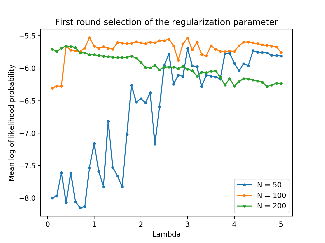
For the numerical analysis of AICM, we focus on a specific customer site with 4 candidate service center locations labeled as (the rank of attractability is unknown). We consider 6 possible scores . We simulate i.i.d. score vectors with some defected ones and use them to fit the AICM. The generation of each score vector is based on the following procedures. First, we simulate a 4-dimensional real vector following the Gaussian distribution with corresponding to the mean score of respectively, and as the covariance matrix. Next, each entry of is rounded to the closest integer from . Finally, with probability 0.8 we accept this score vector, while with probability 0.2 we randomly select an entry of , set it to be zero and accept the resulting score vector. We follow the steps instructed in Section 3.2 to fit the AICM. An essential step is to solve the nonlinear optimization problem (24). This problem is implemented in Julia 1.5.2 (Bezanson et al. 2017) with optimization package JuMP dev (Dunning et al. 2017) as the modeling interface and Ipopt 3.13.2 (Wächter and Biegler 2006) as the solver. For simplicity, we let in (24). We use a 4-fold cross validation approach to select an appropriate regularization parameter . The parameter selection consists of two rounds. The first round is a rough selection, where the candidate is selected from … based on the out-of-sample performance. Suppose is the selected value after the first round. In the second round, we select an optimal from the set based on the out-of-sample performance. The out-of-sample performance is measured by the averaged logarithm of likelihood. The first-round selection results are given in Figure 1 for three different sample sizes . The second-round selection results are given in Table 2, from which we see that the optimal is 2.98, 2.98 and 0.37 for , respectively. The curves in Figure 1 indicate that for a small sample size () a larger regularization parameter lead to a better out-of-sample performance, while for a larger sample size () the best out-of-sample performance is achieved at a smaller regularization parameter. This behavior is intuitive since training the model with a small sample size can lead to over fitting if the model parameters are not sufficiently regularized. When more samples are available to train the model, the regularization can be less restrictive.
Finally, we fit the AICM using samples and the optimal parameter. The probability parameters and from AICM can be used to estimate the probability distribution on scores for each candidate location. The results are given in Figure 2 for the 4 candidate locations. The probability distribution on score values reveal that the rank of attractability from high to low is: Location 3 Location 2 Location 4 Location 1, which matches with the underline stochastic model that generates the scores. The mean scores corresponding to the four locations are given in Table 1.
| Samples | Loc. 1 | Loc. 2 | Loc. 3 | Loc. 4 |
|---|---|---|---|---|
| 50 | 0.83 | 2.79 | 3.86 | 1.67 |
| 100 | 0.88 | 2.91 | 3.89 | 1.87 |
| 200 | 0.87 | 2.88 | 3.94 | 1.78 |
| 50 | 100 | 200 | |
|---|---|---|---|
| range | [2.9, 3.0] | [2.9, 3.0] | [0.3, 0.4] |
| 2.98 | 2.98 | 0.37 |
 (a) Probability distribution on scores of location 1.
 (b) Probability distribution on scores of location 2.
 (c) Probability distribution on scores of location 3.
 (d) Probability distribution on scores of location 4.
4.2 Computational performance of the (DRO-FL) model
We investigate the computational performance of solving numerical instances of the (DRO-FL) model. To generate numerical instances, we create a two-dimensional square as the map. The customer sties are points inside the square, and the coordinates of each customer site are uniformly drawn from the range . We let , which means each customer site can be a candidate location of a service center. We sort the set of distances from small to large, and let be the 5% quantile of the sorted list. For every customer site , we select all customer sites (including ) that are within distance from to form the set . We let the utility completely depend on the distance. Specifically, we set for all . We also let the first element in correspond to utility 5, the last element in correspond to utility 0.5, and any other elements correspond to utility values obtained using a linear interpolation. For a sample , the demand is drawn from the normal distribution . The capacity of each candidate service center is set to be 1000. We assume the cost of opening each service center is identical (an unit cost), and the budget in this case is equivalent to the maximum number of service centers that can be opened. We have generated 18 instances of (DRO-FL), and each instance is characterized by the number of customer sites (also candidate locations) and the budget (number of maximum service centers that can be allocated). For each instance, we have tried three different sample-size options (), and the total variation distance is set to be 0.2 in these calculation. The (DRO-FL) model is implemented and solved using a Gurobi Python interface (Python 3.7 and Gurobi 9.0). For every instance, the master problem and all scenario sub-problems are solved using a single 2.50GHz CPU. The computational results for the 12 instances are shown in Table 3. It is shown that all instances have been solved to optimality within 15 master iterations (see Algorithm 3). The first 9 instances are solved within 120 seconds, and large instances are solved within 1.5 hours where the majority of computational time is spent on the scenario sub-problems. The range of the robust optimal objective is less than 0.7% across three different sample-size options for each instance, and we have also observed that the robust optimal solution remains the same for different sample-size options.
We further investigate the impact of the total variation distance on the robust optimal decision and the objective value. In this study, we focus on the two instances and . For a given sample size (with ), we tune the total variation distance from 0 to 0.4 with an increment 0.05 and investigate the change of optimal objective of (DRO-FL). The results are shown in Figure 3. Obviously, the objective should decrease with as a larger value can allow the worse scenarios get more weight and hence makes the objective decrease. With increasing from 0 to 0.4, the decrement of the objective is 1.5% (1000 units) for the case , and 1.9% (700 units) for the case . The relative decrement is about one magnitude smaller compared to the 10% relative deviation in generating samples for the demand. It is also observed that the optimal decision of (DRO-FL) does not change with the sample size or the total variation distance.
| Obj.() | Iters. | T(s) | Obj() | Iters. | T(s) | Obj() | Iters. | T(s) | ||
|---|---|---|---|---|---|---|---|---|---|---|
| 20 | 3 | 9.60 | 7 | 5.2 | 9.66 | 6 | 5.8 | 9.61 | 6 | 10.2 |
| 20 | 5 | 15.57 | 9 | 2.3 | 15.57 | 7 | 4.8 | 15.6 | 8 | 11.2 |
| 20 | 7 | 22.68 | 6 | 1.6 | 22.55 | 8 | 5.1 | 22.7 | 12 | 17.0 |
| 40 | 5 | 17.52 | 10 | 8.2 | 17.55 | 11 | 17.8 | 17.53 | 10 | 43.4 |
| 40 | 10 | 36.30 | 12 | 9.8 | 36.38 | 9 | 15.9 | 36.34 | 11 | 49.7 |
| 40 | 15 | 54.44 | 11 | 9.2 | 54.46 | 11 | 19.1 | 54.38 | 12 | 55.7 |
| 60 | 10 | 35.74 | 7 | 14.6 | 35.74 | 8 | 36.5 | 35.74 | 6 | 67.5 |
| 60 | 15 | 54.64 | 8 | 17.4 | 54.70 | 10 | 46.8 | 54.70 | 10 | 120.2 |
| 60 | 20 | 67.62 | 8 | 20.2 | 67.70 | 8 | 37.8 | 67.61 | 7 | 84.6 |
| 80 | 15 | 60.62 | 13 | 61.3 | 60.47 | 7 | 74.3 | 60.56 | 6 | 158.1 |
| 80 | 20 | 80.13 | 9 | 41.6 | 80.02 | 8 | 79 | 80.11 | 6 | 136 |
| 80 | 25 | 98.3 | 14 | 70.6 | 98.29 | 14 | 127.5 | 98.38 | 10 | 220.5 |
| 100 | 20 | 78.93 | 10 | 92.5 | 78.90 | 12 | 204.3 | 78.89 | 7 | 293.1 |
| 100 | 25 | 100.69 | 13 | 120 | 100.54 | 11 | 185.5 | 100.53 | 15 | 637.6 |
| 100 | 30 | 117.3 | 15 | 143.9 | 117.16 | 11 | 186.3 | 117.15 | 15 | 694.3 |
| 200 | 40 | 173.24 | 12 | 1092.9 | 173.28 | 7 | 1184 | 173.41 | 11 | 4678.1 |
| 200 | 50 | 215.74 | 13 | 1102.2 | 215.74 | 15 | 2549.9 | 215.78 | 9 | 3829.4 |
| 200 | 60 | 256.8 | 14 | 1214.2 | 256.9 | 8 | 1360.1 | 256.78 | 13 | 5515.9 |


5 Concluding Remarks
The distributionally-robust service center location problem investigated in this research possesses decision-dependent demand induced naturally from a maximum attraction principle and the number of opened service centers in a neighborhood. The ambiguity set considered in this work is a decision-independent one defined using the total-variational distance while many other metics such as the Wasserstein distance, Phi-divergences, etc. can also be applied to define the ambiguity set with minor modification in the formulation. The modeling approach in this work decouples the endogenous impact (decision dependency) and distributional ambiguity. As a result, the model is highly computationally efficient for mid- and large scale instances compared to models with an endogenous uncertainty (ambiguity) set. In practice, such decoupling is likely to be more data driven, as there is a higher chance to identify data-based evidence that supports decision-dependent demand than decision-dependent uncertainty of demand.
Appendix A A cutting-plane algorithm for solving (DRO-FL)
The model (DRO-FL) is a special case of the distributionally-robust two-stage stochastic program with a polyhedral ambiguity set.
Theorem A.1 (Bansal et al. 2018)
Acknowledgments.
The author is grateful to Dr. Liwei Zeng for a valuable discussion on getting an interpretation of the model.References
- Ahmed (2000) Ahmed S (2000) Strategic planning under uncertainty: stochastic integer programming approaches. Ph.D. thesis, University of Illinois at Urbana-Champaign, Urbana, IL, USA.
- Albareda-Sambola et al. (2011) Albareda-Sambola M, Fernández E, da Gama FS (2011) The facility location problem with Bernoulli demands. Omega 39:335–345.
- Bajari and Benkard (2005) Bajari P, Benkard CL (2005) Demand estimation with heterogeneous consumers and unobserved product characteristics: a hedonic approach. Journal of Political Economy 113(6):1239–1276.
- Bansal et al. (2018) Bansal M, Huang KL, Mehrotra S (2018) Decomposition algorithm for two-stage distributionally robust mixed binary programs. SIAM Journal on Optimizaion 28(3):2360–2383.
- Baron and Milner (2010) Baron O, Milner J (2010) Facility location: a robust optimization approach. Production and Operations Management 20(5):772–785.
- Basciftci et al. (2020) Basciftci B, Ahmed S, Shen S (2020) Distributionally robust facility location problem under decision-dependent stochastic demand. https://doi.org/10.1016/j.ejor.2020.11.002.
- Berglund and Kwon (2014) Berglund PG, Kwon C (2014) Robust facility location problem for hazardous waste transportation. Netw. Spat. Econ. 14:91–116.
- Bezanson et al. (2017) Bezanson J, Edelman A, Karpinski S, Shah VB (2017) Julia: A fresh approach to numerical computing. SIAM review 59(1):65–98, URL https://doi.org/10.1137/141000671.
- Chan et al. (2017) Chan T, Shen Z, Siddiq A (2017) Robust defibrillator deployment under cardiac arrest location uncertainty via row-and-column generation. Operations Research 66:358–379.
- Cote and Stephen (2001) Cote M, Stephen T (2001) Four methodologies to improve healthcare demand forecasting. Healthcare Financial Management 55(5):54.
- Doi et al. (2017) Doi S, Ide H, Takeuchi K, Fujita S, Takabayashi K (2017) Estimation and evaluation of future demand and supply of healthcare services based on a patient access area model. International Journal of Environmental Research and Public Health 14(11):1367.
- Döyen et al. (2012) Döyen A, Aras N, Barbarosoğlu G (2012) A two-echelon stochastic facility location model for humanitarian relief logistics. Optim. Lett. 6:1123–1145.
- Dunning et al. (2017) Dunning I, Huchette J, Lubin M (2017) Jump: A modeling language for mathematical optimization. SIAM Review 59(2):295–320, URL http://dx.doi.org/10.1137/15M1020575.
- Goel and Grossmann (2004) Goel V, Grossmann IE (2004) A stochastic programming approach to planning of offshore gas filed developments under uncertainty in reserves. Comp. Chem. Eng. 108:1409–1429.
- Goel and Grossmann (2005) Goel V, Grossmann IE (2005) A Lagrangian duality based branch and bound for solving linear stochastic programs with decision dependent uncertainty. Puigjaner L, Espuña A, eds., European Symposium on Computer Aided Process Engineering-15 (Elsevier Science B. V.).
- Goel and Grossmann (2006) Goel V, Grossmann IE (2006) A class of stochastic programs with decision dependent uncertainty. Math. Program. 108:355–394.
- Goel et al. (2006) Goel V, Grossmann IE, El-Bakry AS, Mulkay EL (2006) A novel branch and bound algorithm for optimal development of gas fields under uncertainty in reserves. Comp. Chem. Eng. 30:1076–1092.
- Gourtani et al. (2020) Gourtani A, Nguyen TD, Xu H (2020) A distributionally robust optimization approach for two-stage facility location problems. EURO Journal on Computational Optimization 8:141–172.
- Griffin et al. (2008) Griffin PM, Scherrer CR, Swann JL (2008) Optimization of community health center locations and service offerings with statistical need estimation. IIE Transactions 40(9):880–892.
- Gülpınar et al. (2013) Gülpınar N, Pachamanova D, Çanakoğlu E (2013) Robust strategies for facility location under uncertainty. European Journal of Operational Research 225:21–35.
- Gupta and Grossmann (2011) Gupta V, Grossmann IE (2011) Solution strategies for multistage stochastic programming with endogenous uncertainty. Comp. Chem. Eng. 35:2235–2247.
- Li et al. (2017) Li Y, Shu J, Song M, Zhang J, Zheng H (2017) Multisourcing supply network design: two-stage chance-constrained model, tractable approximations, and computational results. INFORMS Journal on Computing 29(2):287–300.
- Lim et al. (2013) Lim MK, Bassamboo A, Chopra S, Daskin MS (2013) Facility location decisions with random disruptions and imperfect estimation. Manufacturing & Service Operations Management 15(2):239–249.
- Louveaux and Peeters (1992) Louveaux FV, Peeters D (1992) A dual-based procedure for stochastic facility location. Operations Research 40(3):564–573.
- Luo and Mehrotra (2019a) Luo FQ, Mehrotra S (2019a) Distributionally robust service center location problem with decision dependent utilities. Tech. report, Northwestern University.
- Luo and Mehrotra (2019b) Luo FQ, Mehrotra S (2019b) Service center location problem with decision dependent utilities. https://arxiv.org/pdf/1910.09765.pdf.
- Luo and Mehrotra (2020) Luo FQ, Mehrotra S (2020) Distributionally robust optimization with decision-dependent ambiguity set. Optimization Letters 14:2565–2594.
- Mehrotra et al. (2020) Mehrotra S, Rahimian H, Barah M, Luo FQ, Schantz K (2020) A model of supply-chain decisions for resource sharing with an application to ventilator allocation to combat COVID-19. Naval Research Logistics 67(5):303–320.
- Murali et al. (2012) Murali P, Ordóñez F, Dessouky MM (2012) Facility location under demand uncertainty: response to a large-scale bio-terror attack. Socio-Economic Planning Sciences 46:78–87.
- Nohadani and Roy (2017) Nohadani O, Roy A (2017) Robust optimization with time-dependent uncertainty in radiation therapy. IISE Transactions on Healthcare Systems Engineering 7(2):81–92.
- Nohadani and Sharma (2018) Nohadani O, Sharma K (2018) Optimization under decision-dependent uncertainty. SIAM Journal on Optimization 28(2):1773–1795.
- Noyan et al. (2017) Noyan N, Rudolf G, Lejeune M (2017) Distributionally robust optimization with decision-dependent ambiguity set. http://www.optimization-online.org/DB_FILE/2018/09/6821.pdf.
- Royset and Wets (2017) Royset JO, Wets RJB (2017) Variational theory for optimization under stochastic ambiguity. SIAM Journal on Optimization 27(2):1118–1149.
- Shao et al. (2006) Shao H, Lam WHK, Tam ML (2006) A reliability-based stochastic traffic assignment model for network with multiple user classes under uncertainty in demand. Netw. Spat. Econ. 6:173–204.
- Snyder (2006) Snyder LV (2006) Facility location under uncertainty: a review. IIE Transactions 38:537–554.
- Spacey et al. (2012) Spacey SA, Wiesemann W, Kuhn D, Luk W (2012) Robust software partitioning with multiple instantiation. INFORMS J. Comput. 24(3):500–515.
- Tarhan and Grossmann (2008) Tarhan B, Grossmann IE (2008) A multistage stochastic programming approach with strategies for uncertainty reduction in the synthesis of process networks with uncertain yields. Comp. Chem. Eng. 32:766–788.
- Tarhan et al. (2009) Tarhan B, Grossmann IE, Goel V (2009) Stochastic programming approach for planning of offshore oil or gas field infrastructure under decision-dependent uncertainty. Ind. Eng. Chem. Res. 48:3078–3097.
- Tarhan et al. (2013) Tarhan B, Grossmann IE, Goel V (2013) Computational strategies for non-convex multistage minlp models with decision-dependent uncertainty and gradual uncertainty resolution. Ann. Oper. Res. 203:141–166.
- Tsur and Zemel (2004) Tsur Y, Zemel A (2004) Endangered aquifers: Ggroundwater management under threats of catastrophic events. Water Resources Research 40(W06S20).
- Vayanos et al. (2011) Vayanos P, Kuhn D, Rustem B (2011) Decision rules for information discovery in multi-stage stochastic programming. 50th IEEE Conference on Decision and Control and European Control Conference (CDC-ECC).
- Viswanath et al. (2004) Viswanath K, Peeta S, Salman FS (2004) Investing in the links of a stochastic network to minimize expected shortest path length. Technical report, Purdue University.
- Wächter and Biegler (2006) Wächter A, Biegler LT (2006) On the implementation of a primal-dual interior point filter line search algorithm for large-scale nonlinear programming. Mathematical Programming 106(1):25–57.
- Wang et al. (2002) Wang Q, Batta R, Rump CM (2002) Algorithms for a facility location problem with stochastic customer demand and immobile servers. Annals of Operations Research 111:17–34.