跳到论文正文
W Papers独立论文阅读器 arXiv:2011.12473 论文正文 计算阅读时间 · 0%
引用这篇论文根据当前论文元数据生成,正式投稿前建议核对。


License: CC BY 4.0
arXiv:2011.12473v2 [quant-ph] 26 Oct 2021

Two-level systems with periodic NN-step driving fields: Exact dynamics and quantum state manipulations

Zhi-Cheng Shi Affiliation: Fujian Key Laboratory of Quantum Information and Quantum Optics (Fuzhou University), Fuzhou 350108, China Affiliation: Department of Physics, Fuzhou University, Fuzhou 350108, China    Ye-Hong Chen Affiliation: Theoretical Quantum Physics Laboratory, RIKEN Cluster for Pioneering Research, Wako-shi, Saitama 351-0198, Japan    Wei Qin Affiliation: Theoretical Quantum Physics Laboratory, RIKEN Cluster for Pioneering Research, Wako-shi, Saitama 351-0198, Japan    Yan Xia Thanks: xia-208@163.com Affiliation: Fujian Key Laboratory of Quantum Information and Quantum Optics (Fuzhou University), Fuzhou 350108, China Affiliation: Department of Physics, Fuzhou University, Fuzhou 350108, China    X. X. Yi Thanks: yixx@nenu.edu.cn Affiliation: Center for Quantum Sciences and School of Physics, Northeast Normal University, Changchun 130024, China    Shi-Biao Zheng Affiliation: Fujian Key Laboratory of Quantum Information and Quantum Optics (Fuzhou University), Fuzhou 350108, China Affiliation: Department of Physics, Fuzhou University, Fuzhou 350108, China    Franco Nori Affiliation: Theoretical Quantum Physics Laboratory, RIKEN Cluster for Pioneering Research, Wako-shi, Saitama 351-0198, Japan Affiliation: Department of Physics, University of Michigan, Ann Arbor, Michigan 48109-1040, USA
Abstract

In this work, we derive exact solutions of a dynamical equation, which can represent all two-level Hermitian systems driven by periodic NN-step driving fields. For different physical parameters, this dynamical equation displays various phenomena for periodic NN-step driven systems. The time-dependent transition probability can be expressed by a general formula that consists of cosine functions with discrete frequencies, and, remarkably, this formula is suitable for arbitrary parameter regimes. Moreover, only a few cosine functions (i.e., one to three main frequencies) are sufficient to describe the actual dynamics of the periodic NN-step driven system. Furthermore, we find that a beating in the transition probability emerges when two (or three) main frequencies are similar. Some applications are also demonstrated in quantum state manipulations by periodic NN-step driving fields.

I Introduction

Over the past decade, periodically driven systems have become the focus of intensive research, owing to the appearance of several interesting phenomena, including coherent destruction of tunneling Grossmann et al. 1991; Grifoni and Hänggi 1998, dynamical freezing and localization Broer et al. 2004; Das 2010; Creffield and Platero 2010; Hegde et al. 2014; Nag et al. 2015; Bukov et al. 2015; Agarwala et al. 2016; Luitz et al. 2018; Horstmann et al. 2007; Dai et al. 2018; Choi et al. 2018, etc. Those phenomena are usually inaccessible for undriven systems. More importantly, periodic driving fields can be exploited to control quantum dynamics, and then perform quantum information processing. For instance, multiphoton resonances can be effectively suppressed by periodic driving fields associated with pulse-shaping techniques Gagnon et al. 2017, and sinusoidal driving fields have been used to prepare entangled states and implement quantum gates Paraoanu 2006; Creffield 2007; Li et al. 2008; Li and Paraoanu 2009; Song et al. 2016; Yang et al. 2019. In many-body systems, periodic driving fields also provide a new method for coherent quantum manipulations Eckardt et al. 2005; Eckardt 2017; Sun and Eckardt 2020.

As is well known, it is very challenging to obtain the exact dynamics for the general time-dependent Hamiltonian even in the simplest two-level system (TLS) Barnes and D. Sarma 2012; Zhang et al. 2011; Shevchenko et al. 2012; Stehlik et al. 2012; Gonzalez-Zalba et al. 2016; Rodionov et al. 2016; Vandersypen et al. 2017; Chatterjee et al. 2018; Otxoa et al. 2019; Wen et al. 2020. Exact solutions are only acquired in a handful of special cases, such as the well-known Landau-Zener model Landau 1932; Zener 1932; Shevchenko et al. 2010, Rosen-Zener model Rosen and Zener 1932, Allen-Eberly model Allen and Eberly 1987, etc. The form of the exact solution always contains complicated hypergeometric functions or Γ\Gamma functions.

This similar difficulty also exists in time-dependent periodically driven systems. To study the dynamics of periodically driven systems, one usually uses Floquet theory Shirley 1965; Sambe 1973. The basic idea is to deduce the time-independent Floquet (effective) Hamiltonian and the corresponding micromotion operator, and then acquire the effective dynamical evolution of the periodically driven systems. Therefore, some nontrivial physical properties (e.g., dynamical localization Horstmann et al. 2007; Dai et al. 2018; Choi et al. 2018) can be qualitatively derived. Nevertheless, it is worth mentioning that in the process of obtaining the analytical expressions of the Floquet Hamiltonian, one always makes certain approximations for the system parameters, e.g., the high-frequency limit, the weak-coupling regime, etc. When these approximations do not hold, the effective Hamiltonian of periodically driven systems cannot describe well the actual dynamics.

Recently, a general formalism Goldman and Dalibard 2014, which extends the method introduced in Ref. Rahav et al. 2003, has been proposed to describe periodic-square-wave driven systems Savel'ev and Nori 2002; Cole et al. 2006; Savel’ev et al. 2004; Tonomura 2006; Shi et al. 2016; Ono et al. 2019; Han et al. 2019. More specifically, the dynamics of periodic-square-wave driven systems can be divided into two parts: (i) the long-time-scale dynamics governed by an effective Hamiltonian and (ii) the short-time-scale dynamics governed by a micromotion operator. Nevertheless, this formalism is only suitable for the off-resonant regime (i.e., the frequency of the driving field is off resonant with any energy level separations of the static system) and applicable to a specific square wave that possesses the same time intervals. Then, this method was generalized to the resonant regime Goldman et al. 2015 by performing a time-dependent unitary transformation. However, this approach might also be invalid when the frequency of the driving field is arbitrary.

Until now, for arbitrary parameter regimes, exact and analytical solutions of a periodically driven TLS are still difficult to obtain using nonperturbative approaches. Approximations are often applied in previous works to deal with periodically driven TLSs. For instance, in Ref. Guérin and Jauslin 2003, approximations are needed to obtain the analytical expression of the Floquet Hamiltonian. Here, our goal is to obtain the accurate effective Hamiltonian and the micromotion operator for an arbitrary parameter regime without any approximations. As a result, we manage to describe the exact dynamics at arbitrary time for periodic NN-step driven (PNSD) systems. Moreover, we demonstrate that there are different phenomena in PNSD systems when physical parameters satisfy different conditions, as summarized in Table 1.

Table 1: Various phenomena in periodic NN-step driven systems when physical parameters satisfy different conditions.
Phenomena   Conditions
Coherent destruction of tunneling ϵeff=0\epsilon_{\mathrm{eff}}=0
Complete population transition Δeff=0\Delta_{\mathrm{eff}}=0
Periodic evolution cos𝒩1Θ=1\cos\mathcal{N}_{1}\Theta=1
Stepwise evolution cos𝒩1Θ=0\cos\mathcal{N}_{1}\Theta=0
Population swapping cos⁡Θ=0\cos\Theta=0
Beat phenomenon |ωeff+ωeff−|≫|ωeff−ωeff−||\omega_{\mathrm{eff}}+\omega_{\mathrm{eff}}^{-}|\gg|\omega_{\mathrm{eff}}-\omega_{\mathrm{eff}}^{-}|

In this paper, by deriving the exact expression of the evolution operator, we systematically solve a class of dynamical equations, which can describe all two-level systems driven by periodic NN-step driving fields. Note that the exact solution is valid for the full parameter range since we do not make any approximations. We derive general forms of the amplitudes and phases in the frequency domain. Moreover, we find that there always exist a beat-frequency-like phenomenon in the time-dependent transition probability (hereafter we call it the “beat phenomenon”) in the PNSD system. In particular, the beat phenomenon can also emerge when adopting resonant pulses with different phases. We also demonstrate how to perform phase measurements by using this beat phenomenon.

II Physical model

We consider a two-level system interacting with a driving field. The dynamics is governed by the following Hamiltonian (ℏ=1\hbar=1)

H⁡(t)\displaystyle H(t) =\displaystyle= Υ⁡(t)⋅𝝈+Δ⁡(t)2​𝑰\displaystyle\Upsilon(t)\cdot\bm{\sigma}+\frac{\Delta(t)}{2}\bm{I} (1)
=\displaystyle= Δ(t)|2⟩⟨2|+[ϵ(t)ei​θ​(t)|1⟩⟨2|+H.c.],\displaystyle\Delta(t)|2\rangle\langle 2|+\left[\epsilon(t)e^{i\theta(t)}|1\rangle\langle 2|+\mathrm{H.c.}\right], (3)

where

Υ(t)=(ϵ(t)cosθ(t),ϵ(t)sinθ(t),−Δ(t)/2),\Upsilon(t)=(\epsilon(t)\cos\theta(t),\epsilon(t)\sin\theta(t),-\Delta(t)/2),

𝝈=(σx,σy,σz)\bm{\sigma}=(\sigma_{x},\sigma_{y},\sigma_{z}) represents the Pauli matrices, and 𝑰\bm{I} is the identity matrix. The first and second terms of the second line of Eq. (1) can be regarded as the time-dependent energy bias and tunneling amplitude of the TLS, respectively Grifoni and Hänggi 1998; Shevchenko et al. 2010; Vandersypen et al. 2017; Shevchenko et al. 2012.

We do not restrict the values of Δ⁡(t)\Delta(t), ϵ⁡(t)\epsilon(t), and θ⁡(t)\theta(t) here, so this Hamiltonian can describe all Hermitian quantum systems with a two-level structure. Note that the coefficients Δ⁡(t)\Delta(t), ϵ⁡(t)\epsilon(t), and θ⁡(t)\theta(t) can represent different physical quantities in different systems. For example, Δ⁡(t)\Delta(t) and ϵ⁡(t)\epsilon(t) are the quasiparticle momenta in condensed-matter systems Gagnon et al. 2016; Fillion-Gourdeau et al. 2016; Gagnon et al. 2017, or the detuning and the Rabi frequency in an atomic system interacting with a laser field Scully and Zubairy 1997, or the dc and ac flux biases in superconductor qubits Son et al. 2009; Pan et al. 2017, etc. Without loss of generality, we assume that all coefficients are adjustable, and hereafter we denote Δ⁡(t)\Delta(t), ϵ⁡(t)\epsilon(t), and θ⁡(t)\theta(t) as the detuning, coupling strength, and phase.

The periodic driving field studied here has the form of a repeated NN-step sequence SN:{H1,H2,…,HN}S_{N}:\{H_{1},H_{2},\dots,H_{N}\}. For the nnth step, the interaction time between the TLS and the driving field is τn\tau_{n}, and the Hamiltonian HnH_{n} becomes (n=1,…,Nn=1,\dots,N)

Hn=Δn|2⟩⟨2|+(ϵnei​θn|1⟩⟨2|+H.c.).\displaystyle H_{n}=\Delta_{n}|2\rangle\langle 2|+\left(\epsilon_{n}e^{i\theta_{n}}|1\rangle\langle 2|+\mathrm{H.c.}\right). (4)

Thus, the period of the NN-step sequence is

T=∑n=1Nτn.\displaystyle T=\sum_{n=1}^{N}\tau_{n}. (5)

Note that, for the sake of clarity, the time argument on the parameters are omitted hereafter if these parameters are time independent.

In this work, we also do not restrict the value of each duration τn\tau_{n}. As a result, because no quantities in H⁡(t)H(t) can be treated as perturbations, both the Floquet theory Shirley 1965; Sambe 1973 and the rotating-wave approximation Fuchs et al. 2009; Silveri et al. 2017; Lambert et al. 2018; Shevchenko et al. 2018; Basak et al. 2018 are invalid to calculate the analytical expression of the effective Hamiltonian for this class of systems.

III Effective Hamiltonian and evolution operator

Different from the partitioning introduced in Refs. Rahav et al. 2003; Goldman and Dalibard 2014, we directly divide the evolution operator at arbitrary time t=t′+𝒩​Tt=t^{\prime}+\mathcal{N}T (t′<Tt^{\prime}<T, 𝒩=0,1,2,…\mathcal{N}=0,1,2,\dots) into two factors:

𝕌⁡(t)=𝕌⁡(t′)​𝕌​(𝒩​T)≡exp⁡[−i​ℳ​(t′)]​exp⁡(−i​Heff​𝒩​T).\displaystyle\mathbb{U}(t)=\mathbb{U}(t^{\prime})\mathbb{U}(\mathcal{N}T)\equiv\exp[{-i\mathcal{M}(t^{\prime})}]\exp({-iH_{\mathrm{eff}}\mathcal{N}T}).~~~~ (6)

Physically, the time-dependent micromotion operator ℳ⁡(t′)\mathcal{M}(t^{\prime}) and the time-independent effective Hamiltonian HeffH_{\mathrm{eff}} describe the short (“fast” part) and long (“slow” part) dynamics of the PNSD system, respectively. The eigenvalues of HeffH_{\mathrm{eff}} are referred as the quasienergies of this system.

After some algebraic calculations, we obtain the expression for the micromotion operator ℳ⁡(t′)\mathcal{M}(t^{\prime}) (see Appendix A for details), i.e.,

ℳ(t′)=Δℳ(t′)|2⟩⟨2|+[ϵℳ(t′)ei​θℳ​(t′)|1⟩⟨2|+H.c.],\mathcal{M}(t^{\prime})=\Delta_{\mathcal{M}}(t^{\prime})|2\rangle\langle 2|+\left[\epsilon_{\mathcal{M}}(t^{\prime})e^{i\theta_{\mathcal{M}}(t^{\prime})}|1\rangle\langle 2|+\mathrm{H.c.}\right],~ (7)

where

Δℳ​(t′)\displaystyle\Delta_{\mathcal{M}}(t^{\prime}) =\displaystyle= 2​Bn​(t′)1−An​(t′)2​arccos⁡An​(t′),\displaystyle\frac{2B_{n}(t^{\prime})}{\sqrt{1-A_{n}(t^{\prime})^{2}}}\arccos A_{n}(t^{\prime}),
ϵℳ​(t′)\displaystyle\epsilon_{\mathcal{M}}(t^{\prime}) =\displaystyle= Cn​(t′)2+Dn​(t′)21−An​(t′)2​arccos⁡An​(t′),\displaystyle\frac{{\sqrt{C_{n}(t^{\prime})^{2}+D_{n}(t^{\prime})^{2}}}}{\sqrt{1-A_{n}(t^{\prime})^{2}}}\arccos A_{n}(t^{\prime}),
θℳ​(t′)\displaystyle\theta_{\mathcal{M}}(t^{\prime}) =\displaystyle= arctan⁡Cn​(t′)Dn​(t′).\displaystyle\arctan\frac{C_{n}(t^{\prime})}{D_{n}(t^{\prime})}.

The coefficients An​(t′)A_{n}(t^{\prime}), Bn​(t′)B_{n}(t^{\prime}), Cn​(t′)C_{n}(t^{\prime}), and Dn​(t′)D_{n}(t^{\prime}) satisfy the following relations:

An+1​(t′)\displaystyle A_{n\!+\!1}\!(t^{\prime})\! =\displaystyle= An(τn′)cosEn(t′−τn′)−[𝒜n(τn′)⋅ℰn]sinEn(t′−τn′),\displaystyle\!A_{n}(\tau^{\prime}_{n})\!\cos\!E_{n}(t^{\prime}\!\!-\!\tau^{\prime}_{n})\!-\!\left[\mathcal{A}_{n}\!(\tau^{\prime}_{n})\!\cdot\!\mathcal{E}_{n}\right]\!{\sin\!E_{n}(t^{\prime}\!\!-\!\tau^{\prime}_{n})}, (8)
Bn+1​(t′)\displaystyle B_{n\!+\!1}\!(t^{\prime})\! =\displaystyle= Bn(τn′)cosEn(t′−τn′)+[ℬn(τn′)⋅ℰn]sinEn(t′−τn′),\displaystyle\!B_{n}(\tau^{\prime}_{n})\!\cos\!E_{n}(t^{\prime}\!\!-\!\tau^{\prime}_{n})\!+\!\left[\mathcal{B}_{n}\!(\tau^{\prime}_{n})\!\cdot\!\mathcal{E}_{n}\right]\!{\sin\!E_{n}(t^{\prime}\!\!-\!\tau^{\prime}_{n})}, (10)
Cn+1​(t′)\displaystyle C_{n\!+\!1}\!(t^{\prime})\! =\displaystyle= Cn(τn′)cosEn(t′−τn′)+[𝒞n(τn′)⋅ℰn]sinEn(t′−τn′),\displaystyle\!C_{n}(\tau^{\prime}_{n})\!\cos\!E_{n}(t^{\prime}\!\!-\!\tau^{\prime}_{n})\!+\!\left[\mathcal{C}_{n}\!(\tau^{\prime}_{n})\!\cdot\!\mathcal{E}_{n}\right]\!{\sin\!E_{n}(t^{\prime}\!\!-\!\tau^{\prime}_{n})}, (12)
Dn+1​(t′)\displaystyle D_{n\!+\!1}\!(t^{\prime})\! =\displaystyle= Dn(τn′)cosEn(t′−τn′)+[𝒟n(τn′)⋅ℰn]sinEn(t′−τn′),\displaystyle\!D_{n}(\tau^{\prime}_{n})\!\cos\!E_{n}(t^{\prime}\!\!-\!\tau^{\prime}_{n})\!+\!\left[\mathcal{D}_{n}\!(\tau^{\prime}_{n})\!\cdot\!\mathcal{E}_{n}\right]\!{\sin\!E_{n}(t^{\prime}\!\!-\!\tau^{\prime}_{n})},

where τn−1′<t′<τn′\tau^{\prime}_{n-1}<t^{\prime}<\tau^{\prime}_{n}, and

τn′=∑k=0nτk,τ0′=0,En=ϵn2+Δn2/4.\displaystyle\tau^{\prime}_{n}=\sum\nolimits_{k=0}^{n}\tau_{k},~~~~~~\tau^{\prime}_{0}=0,~~~~~~E_{n}=\sqrt{\epsilon_{n}^{2}+{\Delta_{n}^{2}}/{4}}.

The vectors are

𝒜n​(t′)\displaystyle\mathcal{A}_{n}(t^{\prime}) =\displaystyle= (Dn​(t′),Cn​(t′),Bn​(t′)),\displaystyle(D_{n}(t^{\prime}),C_{n}(t^{\prime}),B_{n}(t^{\prime})),
ℬn​(t′)\displaystyle\mathcal{B}_{n}(t^{\prime}) =\displaystyle= (Cn​(t′),−Dn​(t′),An​(t′)),\displaystyle(C_{n}(t^{\prime}),-D_{n}(t^{\prime}),A_{n}(t^{\prime})),
𝒞n​(t′)\displaystyle\mathcal{C}_{n}(t^{\prime}) =\displaystyle= (−Bn​(t′),An​(t′),Dn​(t′)),\displaystyle(-B_{n}(t^{\prime}),A_{n}(t^{\prime}),D_{n}(t^{\prime})),
𝒟n​(t′)\displaystyle\mathcal{D}_{n}(t^{\prime}) =\displaystyle= (An​(t′),Bn​(t′),−Cn​(t′)),\displaystyle(A_{n}(t^{\prime}),B_{n}(t^{\prime}),-C_{n}(t^{\prime})),
ℰn\displaystyle\mathcal{E}_{n} =\displaystyle= (ϵncosθn,ϵnsinθn,Δn/2)/En.\displaystyle(\epsilon_{n}\cos\theta_{n},\epsilon_{n}\sin\theta_{n},{\Delta_{n}}/{2})/{E_{n}}.

To derive the effective Hamiltonian HeffH_{\mathrm{eff}}, we exploit the definition

𝕌⁡(T)≡exp⁡(−i​Heff​T),\displaystyle\mathbb{U}(T)\equiv\exp{(-iH_{\mathrm{eff}}T)}, (14)

where 𝕌⁡(T)\mathbb{U}(T) is the evolution operator within one period. It is found that HeffH_{\mathrm{eff}} is a special case of the micromotion operator ℳ⁡(t)\mathcal{M}(t), which satisfies Heff=ℳ⁡(T)/TH_{\mathrm{eff}}=\mathcal{M}(T)/T. Thus, HeffH_{\mathrm{eff}} is given by

Heff=Δeff|2⟩⟨2|+(ϵeffei​θeff|1⟩⟨2|+H.c.),\displaystyle H_{\mathrm{eff}}=\Delta_{\mathrm{eff}}|2\rangle\langle 2|+\left(\epsilon_{\mathrm{eff}}e^{i\theta_{\mathrm{eff}}}|1\rangle\langle 2|+\mathrm{H.c.}\right), (15)

where

{Δeff,ϵeff,θeff}={Δℳ​(T),ϵℳ​(T),θℳ​(T)}/T.\{\Delta_{\mathrm{eff}},\epsilon_{\mathrm{eff}},\theta_{\mathrm{eff}}\}=\{\Delta_{\mathcal{M}}(T),\epsilon_{\mathcal{M}}(T),\theta_{\mathcal{M}}(T)\}/T.

From this effective Hamiltonian, one easily finds that the coherent destruction of tunneling (complete population transition) Grossmann et al. 1991; Grifoni and Hänggi 1998 would appear in the PNSD system when ϵeff=0\epsilon_{\mathrm{eff}}=0 (Δeff=0\Delta_{\mathrm{eff}}=0); see Appendix B for details.

Working with 𝕌⁡(t′)\mathbb{U}(t^{\prime}) and 𝕌⁡(T)\mathbb{U}(T), we obtain the exact evolution operator 𝕌⁡(t)\mathbb{U}(t) for the PNSD system, which is expressed as (see Appendix A for details)

𝕌⁡(t)\displaystyle\mathbb{U}(t) =\displaystyle= [A⁡(t)+i​B​(t)C⁡(t)−i​D​(t)−C⁡(t)−i​D​(t)A⁡(t)−i​B​(t)].\displaystyle\left[\begin{array}[]{cc}A(t)+iB(t)&C(t)-iD(t)\\[4.30554pt] -C(t)-iD(t)&A(t)-iB(t)\\ \end{array}\right].

The coefficients A⁡(t)A(t), B⁡(t)B(t), C⁡(t)C(t), and D⁡(t)D(t) are

A⁡(t)\displaystyle A(t) =\displaystyle= An​(t′)​cos⁡𝒩​Θ−[𝒜n​(t′)⋅𝒜NT​(T)]​sin⁡𝒩​Θsin⁡Θ,\displaystyle A_{n}(t^{\prime})\cos\mathcal{N}\Theta-\Big[\mathcal{A}_{n}(t^{\prime})\cdot\mathcal{A}^{\texttt{T}}_{N}(T)\Big]\frac{\sin\mathcal{N}\!\Theta}{\sin\Theta},
B⁡(t)\displaystyle B(t) =\displaystyle= Bn​(t′)​cos⁡𝒩​Θ+[ℬn​(t′)⋅diag⁡{−1,−1,1}⋅𝒜NT​(T)]​sin⁡𝒩​Θsin⁡Θ,\displaystyle B_{n}(t^{\prime})\cos\mathcal{N}\Theta+\Big[\mathcal{B}_{n}(t^{\prime})\cdot\mathrm{diag}\{-1,-1,1\}\cdot\mathcal{A}^{\texttt{T}}_{N}(T)\Big]\frac{\sin\mathcal{N}\Theta}{\sin\Theta},
C⁡(t)\displaystyle C(t) =\displaystyle= Cn​(t′)​cos⁡𝒩​Θ+[𝒞n​(t′)⋅diag⁡{−1,1,−1}⋅𝒜NT​(T)]​sin⁡𝒩​Θsin⁡Θ,\displaystyle C_{n}(t^{\prime})\cos\mathcal{N}\Theta+\Big[\mathcal{C}_{n}(t^{\prime})\cdot\mathrm{diag}\{-1,1,-1\}\cdot\mathcal{A}^{\texttt{T}}_{N}(T)\Big]\frac{\sin\mathcal{N}\Theta}{\sin\Theta},
D⁡(t)\displaystyle D(t) =\displaystyle= Dn​(t′)​cos⁡𝒩​Θ+[𝒟n​(t′)⋅diag⁡{1,−1,−1}⋅𝒜NT​(T)]​sin⁡𝒩​Θsin⁡Θ,\displaystyle D_{n}(t^{\prime})\cos\mathcal{N}\Theta+\Big[\mathcal{D}_{n}(t^{\prime})\cdot\mathrm{diag}\{1,-1,-1\}\cdot\mathcal{A}^{\texttt{T}}_{N}(T)\Big]\frac{\sin\mathcal{N}\Theta}{\sin\Theta},

where Θ=arccos⁡AN​(T)\Theta=\arccos A_{N}(T) and the superscript T denotes the transposition. It is worth mentioning that we make no approximations in obtaining the micromotion operator and the effective Hamiltonian given by Eqs. (7) and (15). Hence, the evolution operator 𝕌⁡(t)\mathbb{U}(t) given by Eq. (III) is exact and valid for the full parameter range.

Note that the evolution operator 𝕌⁡(t)\mathbb{U}(t) given by Eq. (III) is exact at any time, while it is only valid at some specific moments in Ref. Vitanov and Knight 1995. This means that the protocol using rectangular pulses in Ref. Vitanov and Knight 1995 can be regarded as a special case of our results. Additionally, the phenomena of periodic evolution, stepwise evolution, and population swapping can also be observed in PNSD systems when the physical parameters satisfy cos𝒩1Θ=1\cos\mathcal{N}_{1}\Theta=1, cos𝒩1Θ=0\cos\mathcal{N}_{1}\Theta=0, and cos⁡Θ=0\cos\Theta=0, respectively, where 𝒩1\mathcal{N}_{1} is an integer; see Appendix B for details.

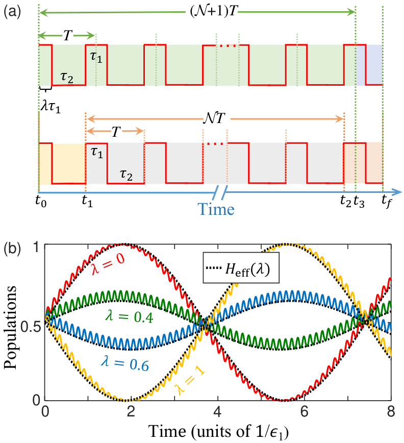
In general situations, the first period of the pulse sequence may have a jump, e.g., from t0t_{0} to t1t_{1} in Fig. 1(a). When this jump is considered, an additional initial kick is needed to describe the dynamics, as discussed in Refs. Rahav et al. 2003; Goldman and Dalibard 2014, because this jump might affect the long-time-scale dynamics [see the solid curve in Fig. 1(b)]. In contrast, we integrate this jump into the effective Hamiltonian here, and do not require an additional kick. The result is that different starting times (phases) of the driving fields would lead to different effective Hamiltonians.

To address this issue more clearly, we employ a quantity λ\lambda to describe this jump [see Fig. 1(a)]. By using another partition of the sequence, we can regard the jump sequence as a complete (N+1)(N+1)-step sequence SN+1:{Hm,Hm+1,…,HN,H1,…,Hm}S_{N+1}:\{H_{m},H_{m+1},\dots,H_{N},H_{1},\dots,H_{m}\}. Here, the final step Hamiltonian is the same to the mmth step Hamiltonian with the interaction time (1−λ)​τ1(1-\lambda)\tau_{1}. Then, we readily obtain the effective Hamiltonian Heff​(λ)H_{\mathrm{eff}}(\lambda) for the jump sequences. It is shown in Fig. 1(b) that the long-time-scale dynamics (i.e., the envelope of the solid curve) caused by different starting times of the driving fields are well described by the effective Hamiltonian Heff​(λ)H_{\mathrm{eff}}(\lambda).

Refer to caption
Figure 1: (a) Schematic diagram of distinct partitions of the same two-step sequence with period TT. The emergence of the first jump is quantified by the parameter λ\lambda. In the top panel, the evolution operator is divided into two factors (shaded with different colors), 𝕌⁡(t,t3)​𝕌​(t3,t0)\mathbb{U}(t,t_{3})\mathbb{U}(t_{3},t_{0}), while it is divided into three factors, 𝕌⁡(t,t2)​𝕌​(t2,t1)​𝕌​(t1,t0)\mathbb{U}(t,t_{2})\mathbb{U}(t_{2},t_{1})\mathbb{U}(t_{1},t_{0}) in the bottom panel. (b) Population evolution of level |2⟩|2\rangle for different λ\lambda, where the initial state is (|1⟩+|2⟩)/2(|1\rangle+|2\rangle)/\sqrt{2}. The black-dotted curves represent the predictions given by the effective Hamiltonian Heff​(λ)H_{\mathrm{eff}}(\lambda). Each dotted curve almost coincides with the envelope of its solid counterpart, indicating that Heff​(λ)H_{\mathrm{eff}}(\lambda) contains relevant information caused by different starting times of the driving fields. The parameters chosen here are {ϵn/ϵ1}={1,2}\{\epsilon_{n}/\epsilon_{1}\}=\{1,2\}, {Δn/ϵ1}={50,40}\{\Delta_{n}/\epsilon_{1}\}=\{50,40\}, and E1​τ1=E2​τ2=π/2E_{1}\tau_{1}=E_{2}\tau_{2}=\pi/2.

IV Analytical expressions for the transition probability

Note that there are two fundamental frequencies in this system: the frequency of the NN-step driving field

ωT=2​π/T,\displaystyle\omega_{T}=2\pi/T, (19)

and the Rabi-like frequency of the effective Hamiltonian

ωeff=ϵeff2+Δeff2/4.\displaystyle\omega_{\mathrm{eff}}=\sqrt{\epsilon_{\mathrm{eff}}^{2}+{\Delta_{\mathrm{eff}}^{2}}/{4}}. (20)

With 𝕌⁡(t)\mathbb{U}(t) in Eq. (III), we can express the time-dependent transition probability P12​(t)P_{12}(t) from the state |1⟩|1\rangle to |2⟩|2\rangle in terms of cosine functions, yielding

P12​(t)=∑l=−∞∞{bl​cos⁡[(2​ωeff+l​ωT)​t−φl]+bl′​cos⁡(l​ωT​t−φl′)},P_{12}(t)\!=\!\!\!\sum_{l=-\infty}^{\infty}\!\!\!\Big\{b_{l}\cos\big[(2\omega_{\mathrm{eff}}+l\omega_{T})t-\varphi_{l}\big]\!+b_{l}^{\prime}\cos\left(l\omega_{T}t\!-\!\varphi_{l}^{\prime}\right)\!\!\Big\}, (21)

where the amplitudes {bl,bl′}\{b_{l},b_{l}^{\prime}\} and the phases {φl,φl′}\{\varphi_{l},\varphi_{l}^{\prime}\} can be obtained by the Fourier transforms (see Appendix C for details):

bl​ei​φl\displaystyle b_{l}e^{i\varphi_{l}} =\displaystyle= limK→∞2K​T​∫0K​TP12​(t)​exp⁡[i⁡(2​ωeff+l​ωT)​t]​𝑑t,\displaystyle\lim_{K\rightarrow\infty}\frac{2}{KT}\int_{0}^{KT}\!\!\!\!P_{12}(t)\exp[i(2\omega_{\mathrm{eff}}+l\omega_{T})t]dt,
bl′​ei​φl′\displaystyle b_{l}^{\prime}e^{i\varphi_{l}^{\prime}} =\displaystyle= limK→∞2K​T​∫0K​TP12​(t)​exp⁡(i​l​ωT​t)​𝑑t.\displaystyle\lim_{K\rightarrow\infty}\frac{2}{KT}\int_{0}^{KT}\!\!\!\!P_{12}(t)\exp(il\omega_{T}t)dt. (22)

From a physical point of view, due to the high-frequency oscillations, most amplitudes {bl,bl′}\{b_{l},b_{l}^{\prime}\} have extremely small values, and thus can be ignored. Therefore, only a few terms in Eq. (21) are kept, but these are sufficient to describe the actual dynamics of the PNSD system at arbitrary times.

IV.1 Example: Two-step sequence

IV.1.1 Expression for the transition probability

Taking the two-step sequence as an example, we can empirically write the expression of the transition probability as

P12​(t)≈P12m​(t)=12​[−(1−λ)​cos⁡2​ωeff​t−λ​cos⁡2​ωeff−​t],P_{12}(t)\!\approx\!P_{12}^{m}(t)\!=\!\frac{1}{2}\Big[1\!-\!(1-\lambda)\cos 2\omega_{\mathrm{eff}}t\!-\!\lambda\cos 2\omega_{\mathrm{eff}}^{-}t\Big], (23)

where we set Δeff=0\Delta_{\mathrm{eff}}=0, and

ωeff−=ωT/2−ωeff,λ=p⁡(1−2​ϑ1​ϑ2).\displaystyle\omega_{\mathrm{eff}}^{-}=\omega_{T}/2-\omega_{\mathrm{eff}},~~~~~~~~~~\lambda=p(1-2\vartheta_{1}\vartheta_{2}).

Here, pp is the maximum transition probability for every Hamiltonian HnH_{n}, and the dynamical phases are ϑn=En​τn/π\vartheta_{n}=E_{n}\tau_{n}/\pi. Note that the focus here is on the dynamical behaviors at arbitrary time rather than some specific moments (e.g., t=𝒩​Tt=\mathcal{N}T) Vitanov and Knight 1995; Garraway and Vitanov 1997. To quantify the validity of Eq. (23) in more detail, we adopt the following definition,

εm​(ts)=1ts​∫0ts|P12​(t)−P12m​(t)|​𝑑t.\displaystyle\varepsilon^{m}(t_{s})=\frac{1}{t_{s}}\int_{0}^{t_{s}}\left|P_{12}(t)-P_{12}^{{m}}(t)\right|dt. (24)

Namely, εm​(ts)\varepsilon^{m}(t_{s}) represents the average error in the time interval [0,ts][0,t_{s}] when adopting P12m​(t)P_{12}^{m}(t) to describe the actual dynamics.

Refer to caption
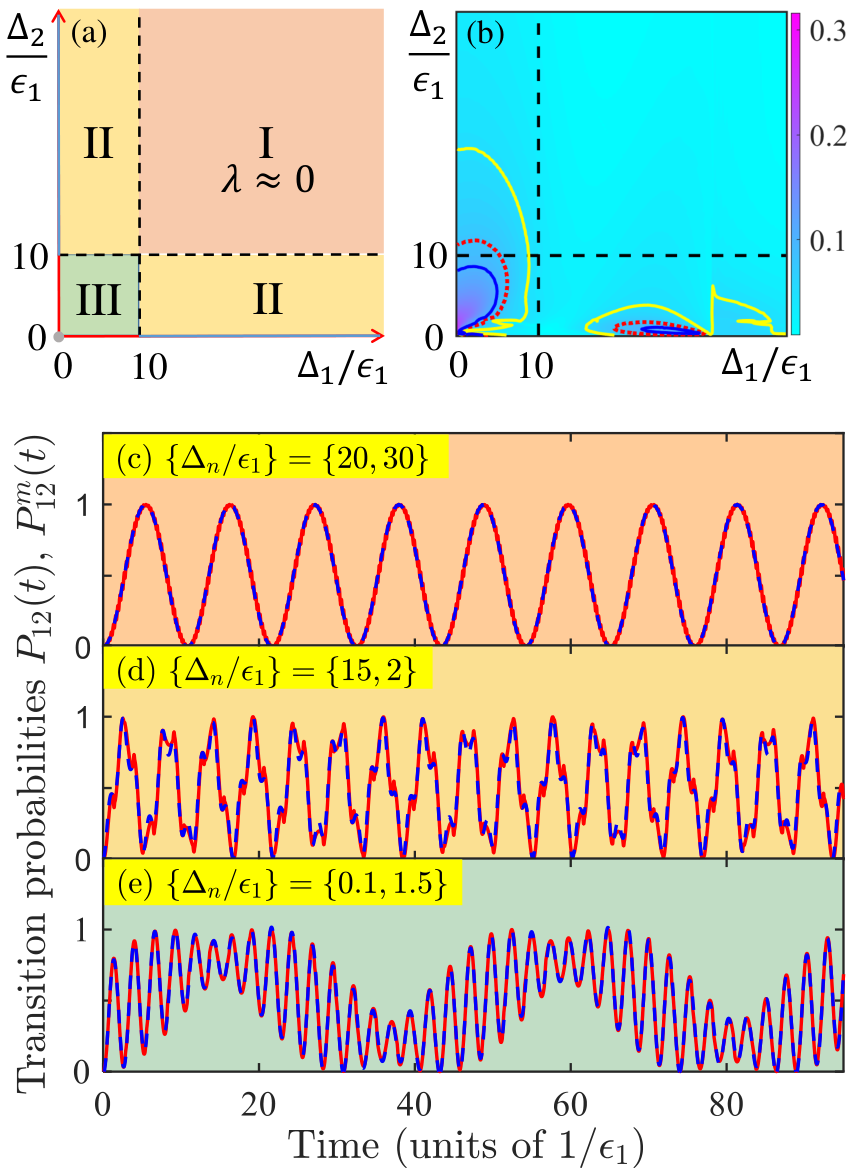
Figure 2: (a) Schematic representation of various parameter regimes. The effective Hamiltonian in Eq. (15) is valid in region I for an arbitrary τ1\tau_{1}. The beat phenomenon can emerge in regions II and III, and is more obvious on the light blue axis or the origin of coordinates (Δ1=0\Delta_{1}=0 or Δ2=0\Delta_{2}=0). (b) εm​(ts)\varepsilon^{m}(t_{s}) vs Δn\Delta_{n}, where {θn}={0,π/3}\{\theta_{n}\}=\{0,\pi/3\}, ϵ2=2​ϵ1\epsilon_{2}=2\epsilon_{1}, τ1=0.2/ϵ1\tau_{1}=0.2/\epsilon_{1}, and τ2\tau_{2} is chosen to be Δeff=0\Delta_{\mathrm{eff}}=0. The yellow solid curves, red dotted curves, and blue solid curves correspond to εm​(ts)=0.05,0.08,0.1\varepsilon^{m}(t_{s})=0.05,0.08,0.1, respectively. The results verify the classification in Fig. 2(a). (c, d) Time-dependent transition probabilities P12​(t)P_{12}(t) and P12m​(t)P_{12}^{m}(t) with different detunings in different regions, where the red solid (blue dashed) curves are plotted by P12​(t)P_{12}(t) [P12m​(t)P_{12}^{m}(t)]. The appreciable overlap between these two curves implies that the actual dynamics at arbitrary time can be well described by P12m​(t)P_{12}^{m}(t). Note that P12m​(t)P_{12}^{m}(t) contains three main frequencies in (e).

We plot εm​(ts)\varepsilon^{m}(t_{s}) as a function of the detuning Δ1\Delta_{1} and Δ2\Delta_{2} in Fig. 2(b), which confirms the classification in Fig. 2(a). To be more specific, in region I of Fig. 2(a), i.e., Δn/ϵn≫1\Delta_{n}/\epsilon_{n}\gg 1, the actual dynamics of the PNSD system can be well described by the effective Hamiltonian (15) and shows Rabi-like oscillations with the frequency ωeff\omega_{\mathrm{eff}}, as shown in Fig. 2(c). Note that most of the previously studied periodically driven systems Ashhab et al. 2007; Tuorila et al. 2010; Neilinger et al. 2016 are in this regime. But, in contrast to those systems, the validity of HeffH_{\mathrm{eff}} does not depend on the frequency of the driving field in this model Silveri et al. 2015; Ivakhnenko et al. 2018. In region II of Fig. 2(a), the effective Hamiltonian (15) is invalid but the actual dynamics can still be well described by Eq. (23), as shown in Fig. 2(d).

Note that Eq. (23) might be invalid in some areas of region III, because εm​(ts)\varepsilon^{m}(t_{s}) is sufficiently large. However, it can be easily solved by including more cosine functions in Eq. (23). For instance, the expression of P12m​(t)P_{12}^{m}(t) keeps three main frequencies (i.e., ωeff\omega_{\mathrm{eff}} and ωeff±=ωT/2±ωeff\omega_{\mathrm{eff}}^{\pm}=\omega_{T}/2\pm\omega_{\mathrm{eff}}) in Fig. 2(e), where the amplitudes and the phases are achieved by Eq. (IV). More examples can be found in Table 2 of Appendix B.

Table 2: The physical parameters in Figs. 6–8 and the corresponding expressions of P12m​(t)P_{12}^{m}(t), where {θn}={0,0}\{\theta_{n}\}=\{0,0\} and ϵ1=ϵ2\epsilon_{1}=\epsilon_{2}.
{ϵ1​τn}\{\epsilon_{1}\tau_{n}\}   {Δn/ϵ1}\{\Delta_{n}/\epsilon_{1}\}   P12m​(t)P_{12}^{m}(t)
Fig. 6(b) {0.0627,0.1092}\{0.0627,0.1092\} {30,40}\{30,40\} 0.25−0.25​cos⁡2​ωeff​t0.25-0.25\cos 2\omega_{\mathrm{eff}}t
Fig. 6(c) {0.0938,0.1748}\{0.0938,0.1748\} {20,25}\{20,25\} 0.4−0.4​cos⁡2​ωeff​t0.4-0.4\cos 2\omega_{\mathrm{eff}}t
Fig. 6(d) {0.0938,0.1464}\{0.0938,0.1464\} {20,30}\{20,30\} 0.5−0.5​cos⁡2​ωeff​t0.5-0.5\cos 2\omega_{\mathrm{eff}}t
Fig. 7(a) {1.6729,0.2066}\{1.6729,0.2066\} {3,2.19}\{3,2.19\} −0.1368​cos⁡(2​ωeff​t−0.3628)−0.28​cos⁡(2​ωeff−​t−0.1416)−0.06​cos⁡2​(ωT​t−0.4846)0.346\!-\!0.1368\cos(2\omega_{\mathrm{eff}}t\!-\!0.3628)\!-\!0.28\cos(2\omega^{-}_{\mathrm{eff}}t\!-\!0.1416)\!-\!0.06\cos 2(\omega_{T}t\!-\!0.4846)
Fig. 7(b) {0.3000,1.6461}\{0.3000,1.6461\} {3,1}\{3,1\} −0.3465​cos⁡(2​ωeff​t−0.1942)+0.0727​cos⁡(2​ωeff−​t+0.54)−0.2256​cos⁡2​(ωeff+​t+0.1519)0.5\!-\!0.3465\cos(2\omega_{\mathrm{eff}}t\!-\!0.1942)\!+\!0.0727\cos(2\omega^{-}_{\mathrm{eff}}t\!+\!0.54)\!-\!0.2256\cos 2(\omega^{+}_{\mathrm{eff}}t\!+\!0.1519)
Fig. 7(c) {0.1535,2.1439}\{0.1535,2.1439\} {3,2}\{3,2\} +0.05357​cos⁡(2​ωeff​t+0.3389)−0.1​cos⁡(2​ωT​t−0.22)−0.1524​cos⁡2​(ωeff+​t+0.1185)0.1972\!+\!0.05357\cos(2\omega_{\mathrm{eff}}t\!+\!0.3389)\!-\!0.1\cos(2\omega_{T}t\!-\!0.22)\!-\!0.1524\cos 2(\omega^{+}_{\mathrm{eff}}t\!+\!0.1185)
Fig. 8(a) {0.3142,3.1377}\{0.3142,3.1377\} {0,40}\{0,40\} 0.5−0.4919​cos⁡(2​ωeff​t+0.2887)+0.05268​cos⁡(2​ωeff−​t−0.5747)−0.04523​cos⁡2​ωeff+​t0.5-0.4919\cos(2\omega_{\mathrm{eff}}t+0.2887)+0.05268\cos(2\omega^{-}_{\mathrm{eff}}t-0.5747)-0.04523\cos 2\omega^{+}_{\mathrm{eff}}t
Fig. 8(b) {0.4126,2.5279}\{0.4126,2.5279\} {0,30}\{0,30\} −0.3241​cos⁡(2​ωeff​t+0.4284)−0.05774​cos⁡(2​ωeff−​t−4.016)−0.04869​cos⁡2​ωeff+​t0.3375\!-\!0.3241\cos(2\omega_{\mathrm{eff}}t+0.4284)\!-\!0.05774\cos(2\omega^{-}_{\mathrm{eff}}t-4.016)\!-\!0.04869\cos 2\omega^{+}_{\mathrm{eff}}t
Fig. 8(c) {0.2328,1.5191}\{0.2328,1.5191\} {0,50}\{0,50\} −0.1873​cos⁡(2​ωeff​t+0.3242)+0.02425​cos⁡(2​ωeff−​t−0.7375)−0.02175​cos⁡2​ωeff+​t0.1916\!-\!0.1873\cos(2\omega_{\mathrm{eff}}t+0.3242)\!+\!0.02425\cos(2\omega^{-}_{\mathrm{eff}}t-0.7375)\!-\!0.02175\cos 2\omega^{+}_{\mathrm{eff}}t
Fig. 8(d) {1.5708,3.1377}\{1.5708,3.1377\} {0,40}\{0,40\} −0.6189​cos⁡(2​ωeff​t+1.048)−0.06237​cos⁡(2​ωeff+​t+ωT​t−1.044)+0.1667​cos⁡2​ωeff+​t0.5\!-\!0.6189\cos(2\omega_{\mathrm{eff}}t+1.048)\!-\!0.06237\cos(2\omega^{+}_{\mathrm{eff}}t+\omega_{T}t-1.044)\!+\!0.1667\cos 2\omega^{+}_{\mathrm{eff}}t

IV.1.2 Beat phenomenon in the transition probability

Figure 2(b) clearly demonstrates that the actual dynamics of the PNSD two-level system can be well described by a superposition of two cosine functions in region II. An interesting finding is that when the sum of the frequencies of these two cosine functions is much greater than their difference, i.e., |ωeff+ωeff−|≫|ωeff−ωeff−||\omega_{\mathrm{eff}}+\omega_{\mathrm{eff}}^{-}|\gg|\omega_{\mathrm{eff}}-\omega_{\mathrm{eff}}^{-}|, we can observe a beat phenomenon in the transition probability P12​(t)P_{12}(t), as shown in Figs. 3(a) and 3(b). In particular, this beat phenomenon can also emerge for resonant pulses with different phases [the light gray dot in Fig. 2(a)], as shown in Figs. 3(c) and 3(d). Furthermore, Figs. 3(e) and 3(f) demonstrate that the beat phenomenon emerges in region III of Fig. 2(a), where P12m​(t)P_{12}^{m}(t) contains three cosine functions (i.e., three similar main frequencies ωeff\omega_{\mathrm{eff}} and ωeff±\omega_{\mathrm{eff}}^{\pm}).

Figure 3: Time-dependent transition probabilities P12​(t)P_{12}(t) and P12m​(t)P_{12}^{m}(t), which show distinct beat phenomena in different regions of Fig. 2(a). The red solid (blue dashed) curves are plotted by P12​(t)P_{12}(t) [P12m​(t)P_{12}^{m}(t)], and the appreciable overlap between these two curves shows the validity of Eq. (23). Note that P12m​(t)P_{12}^{m}(t) contains three main frequencies in (e) and (f).

Physically, this beat phenomenon results from the interference of the phases (ϑn\vartheta_{n} or θn\theta_{n}), which is different from previous works, where the quantum beat originates from the interference between different transition channels Haroche 1976; Lefebvre-Brion and Field 2004; Gu et al. 2011. The beat phenomenon cannot be explained by only using the effective Hamiltonian, because the micromotion operator ℳ⁡(t′)\mathcal{M}(t^{\prime}) plays a key role in the transition process. Furthermore, the beat phenomenon only emerges in some special physical regimes [e.g., regions II and III in Fig. 2(a)], where the traditional methods, such as the Floquet theory Grifoni and Hänggi 1998; Shirley 1965; Sambe 1973 and the rotating-wave approximation Fuchs et al. 2009; Silveri et al. 2017; Lambert et al. 2018; Shevchenko et al. 2018; Basak et al. 2018, might not hold.

IV.2 Beat phenomenon in periodic NN-step driven systems

According to Eq. (23), the beat phenomenon is more obvious when λ=1/2\lambda=1/2, as shown in Fig. 3(b). Actually, this is the case where the beating always exists in the PNSD system, when at least one Hamiltonian is in the largely detuned (resonant) regime; see Appendix D for details. By modulating the dynamical phases, the transition probability of the PNSD system can be approximately given by

P12b​(t)=12​[sin2⁡ϖ1​(t−tp)+sin2⁡ϖ1′​(t−tp)],\displaystyle P_{12}^{{b}}(t)=\frac{1}{2}\left[\sin^{2}\varpi_{1}(t-t_{p})+\sin^{2}\varpi_{1}^{\prime}(t-t_{p})\right], (25)

where two similar main frequencies ϖ1\varpi_{1} and ϖ1′\varpi_{1}^{\prime} are closely related to the effective quantity ωeff\omega_{\mathrm{eff}}, and tpt_{p} is the time-shifting factor. Moreover, the parity number of NN determines the values of the frequencies ϖ1\varpi_{1} and ϖ1′\varpi_{1}^{\prime}. To be specific, when there are n1n_{1} Hamiltonians in the resonant regime, we have

ϖ1=12​{[n1−(−1)N]​ωeff−+[n1+(−1)N]​ωeff,odd​n1n1​ωeff−+[n1−2​(−1)N]​ωeff,even​n1\varpi_{1}\!=\!\frac{1}{2}\!\left\{\begin{array}[]{ll}{\!\!\left[n_{1}\!-\!(-1)^{N}\right]\omega^{-}_{\mathrm{eff}}}\!+\!\left[n_{1}\!+\!(-1)^{N}\right]\omega_{\mathrm{eff}},&\textrm{odd}~n_{1}\\[6.45831pt] {\!\!n_{1}\omega^{-}_{\mathrm{eff}}+\left[n_{1}\!-\!2(-1)^{N}\right]\omega_{\mathrm{eff}}},&\textrm{even}~n_{1}\\ \end{array}\right.

and

ϖ1′=12​{(n1+1)​ωeff−+[n1−2​(−1)N+1]​ωeff,odd​n1[n1−(−1)N+1]​ωeff−+[n1+(−1)N+1]​ωeff,even​n1.\varpi_{1}^{\prime}\!=\!\frac{1}{2}\!\left\{\begin{array}[]{ll}{\!\!(n_{1}+1)\omega^{-}_{\mathrm{eff}}+\left[n_{1}\!-\!2(-1)^{N}\!+\!1\right]\omega_{\mathrm{eff}}},&\textrm{odd}~n_{1}\\[6.45831pt] {\!\!\left[n_{1}\!-\!(\!-\!1)^{N}\!\!\!+\!1\right]\!\omega^{-}_{\mathrm{eff}}\!+\!\!\left[n_{1}\!+\!(\!-\!1)^{N}\!\!\!+\!1\right]\!\omega_{\mathrm{eff}}},&\textrm{even}~n_{1}.\\ \end{array}\right.

V Applications in quantum state manipulations

Figure 4: Time-dependent transition probability P12​(t)P_{12}(t) in the case of an unknown phase in the two-step driven system, where other parameters are θ1=0\theta_{1}=0, ϵ1=ϵ2\epsilon_{1}=\epsilon_{2}, {Δn/ϵ1}={0,40}\{\Delta_{n}/\epsilon_{1}\}=\{0,40\}, and ϑn=1/2\vartheta_{n}=1/2. The red solid curves represent the actual dynamics and the green (black) dashed envelope curves are described by the functions Pb(t)=1/2(1±cosωbt)P_{b}(t)=1/2(1\pm\cos\omega_{b}t). According to the envelope waveform of P12​(t)P_{12}(t), we can acquire the beat frequency ωb\omega_{b} by the green (black) dashed envelope curves. Different ωb\omega_{b} reflect different phases, given by Eq. (26).

The beat phenomenon observed in the PNSD system could find potential applications in homodyne detection, such as phase measurements. Taking the two-step sequence as an example, we assume that the physical parameters {Δn,ϵn}\{\Delta_{n},\epsilon_{n}\} are given and the phase θn\theta_{n} is unknown. Then, each duration can be chosen to be τn=π/2​En\tau_{n}=\pi/2E_{n}. In this situation, the beating in the transition probability would appear in this system, as shown in Fig. 4. According to Eq. (25), the physical parameters are closely interconnected, and have the relations (N=2N=2)

ωb=ϖ1′−ϖ1≈2​ϵ2T​E2​cos⁡(θ1−θ2).\displaystyle\omega_{b}=\varpi_{1}^{\prime}-\varpi_{1}\approx\frac{2\epsilon_{2}}{TE_{2}}\cos(\theta_{1}-\theta_{2}). (26)

Thus, we can map the phase θn\theta_{n} onto the beat frequency, enabling it to be easily measured by detecting the envelope waveform of the beat signal.

In Fig. 4, we illustrate the time-dependent transition probability in the case of an unknown phase. These results demonstrate that the dynamical behaviors are different and we can acquire the beat frequency ωb\omega_{b} by population measurements. Then, by inversely solving Eq. (26), one can obtain the phase of the system.

Refer to caption
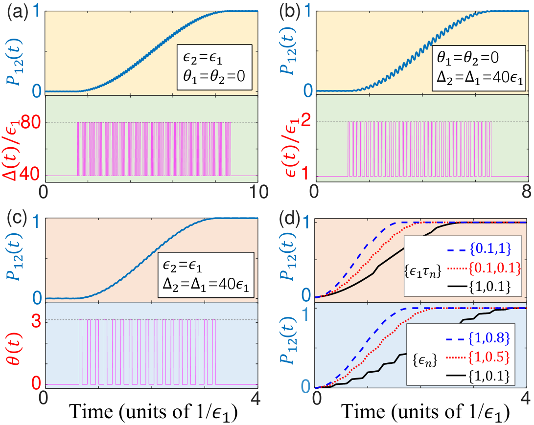
Figure 5: Time-dependent transition probability P12​(t)P_{12}(t) and the corresponding waveform of physical quantities: (a) detuning modulation, (b) coupling strength modulation, and (c) phase modulation. In (a), (b), and (c), by merely modulating one parameter with a square-wave sequence, we achieve the population inversion in the TLS, respectively. (d) Population inversion by merely modulating {τn}\{\tau_{n}\} (upper panel, ϵ2=ϵ1/2\epsilon_{2}=\epsilon_{1}/2) or ϵ2\epsilon_{2} (lower panel, {τn}={0.1,0.2}/ϵ1\{\tau_{n}\}=\{0.1,0.2\}/\epsilon_{1}). Panel (d) shows that the transition time is adjustable by choosing different quantities in the resonant pulses.

The periodic NN-step driving field can be widely used in quantum coherent control, since all physical quantities can be exploited to manipulate quantum states. For example, to implement the complete transition from |1⟩|1\rangle to |2⟩|2\rangle, we can adopt multiple choices to design physical parameters in the PNSD system, such as the detuning Δ⁡(t)\Delta(t) [see the bottom panel of Fig. 5(a)], the coupling strength ϵ⁡(t)\epsilon(t) [see the bottom panel of Fig. 5(b)], or the phase θ⁡(t)\theta(t) [see the bottom panel of Fig. 5(c)].

This method is particularly useful for complicated quantum systems. Furthermore, for resonant pulses with different coupling strengths, the total evolution time of the complete transition reads

𝕋=π⁡(τ1+τ2)2​(ϵ1​τ1+ϵ2​τ2),τn<π2​ϵn,n=1,2.\displaystyle\mathbb{T}=\frac{\pi(\tau_{1}+\tau_{2})}{2(\epsilon_{1}\tau_{1}+\epsilon_{2}\tau_{2})},~~~\tau_{n}<\frac{\pi}{2\epsilon_{n}},~~~n=1,2. (27)

Here, π/2​ϵ1≤𝕋≤π/2​ϵ2{\pi}/{2\epsilon_{1}}\leq\mathbb{T}\leq{\pi}/{2\epsilon_{2}}, when ϵ2<ϵ1\epsilon_{2}<\epsilon_{1}. By modulating the interaction time τn\tau_{n} or the coupling strength ϵn\epsilon_{n}, we can control the transition time from |1⟩|1\rangle to |2⟩|2\rangle, as shown in Fig. 5(d).

Finally, the coherent destruction of tunneling phenomenon in PNSD systems offers us a possible way to implement the forbidden transition by resonant pulses. The physical parameters should satisfy θ2=θ1+π\theta_{2}=\theta_{1}+\pi and ϵ2​τ2=ϵ1​τ1≪π/2\epsilon_{2}\tau_{2}=\epsilon_{1}\tau_{1}\ll{\pi}/{2}.

VI Conclusion

We have presented the exact solution of the evolution operator for the full parameter range in the periodic NN-step driven TLS. Then, we display different physical parameter regimes for various phenomena in this system, including the well-known coherent destruction of tunneling, complete population transition, and beat phenomenon.

The time-dependent transition probability of the PNSD system can be expanded by a few cosine functions with discrete frequencies. Generally speaking, no more than three main frequencies are needed to describe the actual dynamics of the PNSD system. In addition, we derive the exact expression of the effective Hamiltonian of the PNSD system, which is valid in the largely detuned regime (i.e., Δn/ϵn≫1\Delta_{n}/\epsilon_{n}\gg 1) or the high-frequency limit. When the micromotion operator contributes to the evolution, the effective Hamiltonian would be invalid. For this situation, we introduce a modified transition probability to describe the actual dynamics.

Moreover, we have demonstrated that the beat phenomenon always exists in the NN-step driven TLS, which cannot be explained by only the effective Hamiltonian. We have also described the beat phenomenon by the resonant pulses with different phases in the PNSD system, and given the general expressions of two similar frequencies when N>2N>2. The beat phenomenon originates from the interference of the phases and can be helpful for a driven quantum TLS used in quantum state manipulations.

Acknowledgements.
We acknowledge helpful discussions with Dr. S. N. Shevchenko and Dr. Y. K. Jiang. This work is supported by the National Natural Science Foundation of China under Grant No. 11805036, No. 11674060, No. 11534002, and No. 11775048, the Natural Science Funds for Distinguished Young Scholar of Fujian Province under Grant No. 2020J06011, and the Project from Fuzhou University under Grant No. JG202001-2. Y.-H.C. is supported by the Japan Society for the Promotion of Science (JSPS) KAKENHI Grant No. JP19F19028. F.N. is supported in part by: Nippon Telegraph and Telephone Corporation (NTT) Research, the Japan Science and Technology Agency (JST) [via the Quantum Leap Flagship Program (Q-LEAP), the Moonshot R&D Grant No. JPMJMS2061, and the Centers of Research Excellence in Science and Technology (CREST) Grant No. JPMJCR1676], the Japan Society for the Promotion of Science (JSPS) [via the Grants-in-Aid for Scientific Research (KAKENHI) Grant No. JP20H00134 and the JSPS–RFBR Grant No. JPJSBP120194828], the Army Research Office (ARO) (Grant No. W911NF-18-1-0358), the Asian Office of Aerospace Research and Development (AOARD) (via Grant No. FA2386-20-1-4069), and the Foundational Questions Institute Fund (FQXi) via Grant No. FQXi-IAF19-06.

Appendix A Solutions for the dynamical equation in periodic NN-step driven two-level systems

A.1 General formalism

The physical model we consider here is a two-level system (TLS) driven by a periodic NN-step driving field. The general form of its Hamiltonian reads (ℏ=1\hbar=1)

H⁡(t)\displaystyle H(t) =\displaystyle= ∑k=0𝒩∑n=1NHn​[ζ⁡(t−k​T−∑m=0n−1τm)−ζ⁡(t−k​T−∑m=0nτm)],\displaystyle\sum_{k=0}^{\mathcal{N}}\sum_{n=1}^{N}H_{n}\left[\zeta\left(t-kT-\sum_{m=0}^{n-1}\tau_{m}\right)-\zeta\left(t-kT-\sum_{m=0}^{n}\tau_{m}\right)\right],
Hn\displaystyle H_{n} =\displaystyle= Δn​|2⟩​⟨2|+ϵn​exp⁡(i​θn)|1⟩​⟨2|+H.c.,\displaystyle\Delta_{n}|2\rangle\langle 2|+\epsilon_{n}\exp({i\theta_{n}})|1\rangle\langle 2|+\mathrm{H.c.}, (28)

where ζ⁡(t)\zeta(t) is the Heaviside function, τ0=0\tau_{0}=0, τn\tau_{n} (n=1,…,Nn=1,\dots,N) is the interaction time between the TLS and the nnth-step driving field, and T=τN+τN−1+⋯+τ1T=\tau_{N}+\tau_{N-1}+\cdots+\tau_{1} is the period of the NN-step sequence.

Generally speaking, the evolution operator of periodically driven systems can be divided into two parts:

𝕌⁡(t)=ℙ⁡(t)​exp⁡(−i​Heff​t),\displaystyle\mathbb{U}(t)=\mathbb{P}(t)\exp({-iH_{\mathrm{eff}}t}), (29)

where the unitary operator ℙ⁡(t)\mathbb{P}(t) has the same period as the system Hamiltonian. The eigenvalues of the effective Hamiltonian HeffH_{\mathrm{eff}} are referred to as the quasienergies of the system. Different from both this partitioning and the partition introduced in Refs. Rahav et al. 2003; Goldman and Dalibard 2014, we directly divide the evolution operator of a periodic NN-step driven system at arbitrary final time t=t′+𝒩​Tt=t^{\prime}+\mathcal{N}T (t′<Tt^{\prime}<T, 𝒩=1,2,…\mathcal{N}=1,2,\dots) into two parts:

𝕌⁡(t)=𝕌⁡(t′)​𝕌(T)⋯𝕌(T)⏟𝒩=𝕌⁡(t′)​𝕌​(𝒩​T)≡exp⁡[−i​ℳ​(t′)]​exp⁡(−i​Heff​𝒩​T),\displaystyle\mathbb{U}(t)=\mathbb{U}(t^{\prime})\underbrace{\mathbb{U}(T)\cdots\mathbb{U}(T)}_{\mathcal{N}}=\mathbb{U}(t^{\prime})\mathbb{U}(\mathcal{N}T)\equiv\exp[{-i\mathcal{M}(t^{\prime})}]\exp({-iH_{\mathrm{eff}}\mathcal{N}T}), (30)

where

𝕌(T)=UN(τN)UN−1(τN−1)⋯U1(τ1)≡exp(−iHeffT)\mathbb{U}(T)=U_{N}(\tau_{N})U_{N-1}(\tau_{N-1})\cdots U_{1}(\tau_{1})\equiv\exp({-iH_{\mathrm{eff}}T})

is the evolution operator within one period. Un​(t′)=exp⁡(−i​Hn​t′)U_{n}(t^{\prime})=\exp({-iH_{n}t^{\prime}}) represents the evolution operator for the nnth Hamiltonian, n=1,…,Nn=1,\dots,N. Physically, the time-dependent micromotion operator ℳ⁡(t′)\mathcal{M}(t^{\prime}) describes the short-time-scale (“fast” part) dynamics of the system, and the time-independent effective Hamiltonian HeffH_{\mathrm{eff}} describes the long-time-scale (“slow” part) dynamics of the system.

In order to derive the expression of the evolution operator 𝕌⁡(t)\mathbb{U}(t) for the periodic NN-step driven system, we need to calculate both the micromotion operator ℳ⁡(t′)\mathcal{M}(t^{\prime}) and the effective Hamiltonian HeffH_{\mathrm{eff}}. To be specific, the micromotion operator ℳ⁡(t′)=Δℳ​(t′)​|2⟩​⟨2|+ϵℳ​(t′)​exp⁡[i​θℳ​(t′)]|1⟩​⟨2|+H.c.\mathcal{M}(t^{\prime})=\Delta_{\mathcal{M}}(t^{\prime})|2\rangle\langle 2|+\epsilon_{\mathcal{M}}(t^{\prime})\exp[{i\theta_{\mathcal{M}}(t^{\prime})}]|1\rangle\langle 2|+\mathrm{H.c.} is defined by the evolution operator 𝕌⁡(t′)\mathbb{U}(t^{\prime}), such that

exp⁡[−i​ℳ​(t′)]≡𝕌⁡(t′)={U1​(t′),t′∈[0,τ1]U2​(t′−τ1)​U1​(τ1),t′∈(τ1,τ2+τ1]U3​(t′−τ2−τ1)​U2​(τ2)​U1​(τ1),t′∈(τ2+τ1,τ3+τ2+τ1]⋯⋯UN(t′−∑k=1N−1τk)UN−1(τN−1)⋯U2(τ2)U1(τ1),t′∈(∑k=1N−1τk,∑k=1Nτk],\displaystyle\exp[{-i\mathcal{M}(t^{\prime})}]\equiv\mathbb{U}(t^{\prime})=\left\{\begin{array}[]{lllll}U_{1}(t^{\prime}),&t^{\prime}\in[0,\tau_{1}]\\[3.01385pt] U_{2}(t^{\prime}-\tau_{1})U_{1}(\tau_{1}),&t^{\prime}\in(\tau_{1},\tau_{2}+\tau_{1}]\\[3.01385pt] U_{3}(t^{\prime}-\tau_{2}-\tau_{1})U_{2}(\tau_{2})U_{1}(\tau_{1}),&t^{\prime}\in(\tau_{2}+\tau_{1},\tau_{3}+\tau_{2}+\tau_{1}]\\[3.01385pt] \cdots&\cdots\\[3.01385pt] U_{N}(t^{\prime}-\sum\nolimits_{k=1}^{N-1}\tau_{k})U_{N-1}(\tau_{N-1})\cdots U_{2}(\tau_{2})U_{1}(\tau_{1}),&t^{\prime}\in(\sum\nolimits_{k=1}^{N-1}\tau_{k},\sum\nolimits_{k=1}^{N}\tau_{k}],\\[3.01385pt] \end{array}\right.

where Un​(t′)=exp⁡(−i​Hn​t′)U_{n}(t^{\prime})=\exp{(-iH_{n}t^{\prime})}.

When t′∈[0,τ1]t^{\prime}\in[0,\tau_{1}], the evolution operator becomes

𝕌⁡(t′)=U1​(t′)=[cos⁡(E1​t′)+i​Δ12​E1​sin⁡(E1​t′)−i​ϵ1​ei​θ1E1​sin⁡(E1​t′)−i​ϵ1​e−i​θ1E1​sin⁡(E1​t′)cos⁡(E1​t′)−i​Δ12​E1​sin⁡(E1​t′)]=[A1​(t′)+i​B1​(t′)C1​(t′)−i​D1​(t′)−C1​(t′)−i​D1​(t′)A1​(t′)−i​B1​(t′)].\displaystyle\mathbb{U}(t^{\prime})\!=\!U_{1}(t^{\prime})\!=\!\!\left[\!\!\begin{array}[]{cc}\displaystyle\cos(E_{1}t^{\prime})+i\frac{\Delta_{1}}{2E_{1}}\sin(E_{1}t^{\prime})&\displaystyle-i\frac{\epsilon_{1}e^{i\theta_{1}}}{E_{1}}\sin(E_{1}t^{\prime})\\[8.61108pt] \displaystyle-i\frac{\epsilon_{1}e^{-i\theta_{1}}}{E_{1}}\sin(E_{1}t^{\prime})&\displaystyle\cos(E_{1}t^{\prime})-i\frac{\Delta_{1}}{2E_{1}}\sin(E_{1}t^{\prime})\\ \end{array}\!\!\right]\!\!=\!\!\left[\!\!\begin{array}[]{cc}A_{1}(t^{\prime})+iB_{1}(t^{\prime})&C_{1}(t^{\prime})-iD_{1}(t^{\prime})\\[4.30554pt] -C_{1}(t^{\prime})-iD_{1}(t^{\prime})&A_{1}(t^{\prime})-iB_{1}(t^{\prime})\\ \end{array}\!\!\right]\!\!.~~~~~~

Comparing the left-hand side and the right-hand side of Eq. (A.1), we find

A1​(t′)=cos⁡(E1​t′),B1​(t′)=Δ12​E1​sin⁡(E1​t′),C1​(t′)=ϵ1sinθ1E1​sin⁡(E1​t′),D1​(t′)=ϵ1cosθ1E1​sin⁡(E1​t′),A_{1}(t^{\prime})=\cos(E_{1}t^{\prime}),~~~~~\ B_{1}(t^{\prime})=\frac{\Delta_{1}}{2E_{1}}\sin(E_{1}t^{\prime}),~~~~~\ C_{1}(t^{\prime})=\frac{\epsilon_{1}\sin\theta_{1}}{E_{1}}\sin(E_{1}t^{\prime}),~~~~~\ D_{1}(t^{\prime})=\frac{\epsilon_{1}\cos\theta_{1}}{E_{1}}\sin(E_{1}t^{\prime}),

where E1=ϵ12+Δ12/4E_{1}=\sqrt{\epsilon_{1}^{2}+{\Delta_{1}^{2}}/{4}}. Then, by inversely solving the equation exp⁡[−i​ℳ​(t′)]=𝕌⁡(t′)\exp{[-i\mathcal{M}(t^{\prime})]}=\mathbb{U}(t^{\prime}), we have

Δℳ​(t′)=2​B1​(t′)1−A1​(t′)2​arccos⁡A1​(t′),ϵℳ​(t′)=C1​(t′)2+D1​(t′)21−A1​(t′)2​arccos⁡A1​(t′),θℳ​(t′)=arctan⁡C1​(t′)D1​(t′).\Delta_{\mathcal{M}}(t^{\prime})=\frac{2B_{1}(t^{\prime})}{\sqrt{1-A_{1}(t^{\prime})^{2}}}\arccos A_{1}(t^{\prime}),~~~~~\ \epsilon_{\mathcal{M}}(t^{\prime})=\frac{\sqrt{C_{1}(t^{\prime})^{2}+D_{1}(t^{\prime})^{2}}}{\sqrt{1-A_{1}(t^{\prime})^{2}}}\arccos A_{1}(t^{\prime}),~~~~~\ \theta_{\mathcal{M}}(t^{\prime})=\arctan\frac{C_{1}(t^{\prime})}{D_{1}(t^{\prime})}.

Similarly, when t′∈(τ1,τ2+τ1]t^{\prime}\in(\tau_{1},\tau_{2}+\tau_{1}], the evolution operator is

𝕌⁡(t′)\displaystyle\mathbb{U}(t^{\prime}) =\displaystyle= U2​(t′−τ1)​U1​(τ1)=exp⁡[−i​H2​(t′−τ1)]​exp⁡(−i​H1​τ1)\displaystyle U_{2}(t^{\prime}-\tau_{1})U_{1}(\tau_{1})=\exp[{-iH_{2}(t^{\prime}-\tau_{1})}]\exp({-iH_{1}\tau_{1}}) (42)
=\displaystyle= [cosE2(t′−τ1)+iΔ22​E2sinE2(t′−τ1)−iϵ2​ei​θ2E2sinE2(t′−τ1)−iϵ2​e−i​θ2E2sinE2(t′−τ1)cosE2(t′−τ1)−iΔ22​E2sinE2(t′−τ1)]⋅[A1​(τ1)+i​B1​(τ1)C1​(τ1)−i​D1​(τ1)−C1​(τ1)−i​D1​(τ1)A1​(τ1)−i​B1​(τ1)]\displaystyle\!\!\left[\!\begin{array}[]{cc}\displaystyle\cos E_{2}(t^{\prime}\!\!-\!\tau_{1})+i\frac{\Delta_{2}}{2E_{2}}\sin E_{2}(t^{\prime}\!\!-\!\tau_{1})&\displaystyle-i\frac{\epsilon_{2}e^{i\theta_{2}}}{E_{2}}\sin E_{2}(t^{\prime}-\tau_{1})\\[4.30554pt] \displaystyle-i\frac{\epsilon_{2}e^{-i\theta_{2}}}{E_{2}}\sin E_{2}(t^{\prime}-\tau_{1})&\!\!\!\!\!\!\displaystyle\cos E_{2}(t^{\prime}\!\!-\!\tau_{1})-i\frac{\Delta_{2}}{2E_{2}}\sin E_{2}(t^{\prime}\!\!-\!\tau_{1})\\ \end{array}\!\!\!\right]\!\!\cdot\!\!\left[\!\!\begin{array}[]{cc}A_{1}(\tau_{1})+iB_{1}(\tau_{1})&C_{1}(\tau_{1})-iD_{1}(\tau_{1})\\[4.30554pt] -C_{1}(\tau_{1})-iD_{1}(\tau_{1})&A_{1}(\tau_{1})-iB_{1}(\tau_{1})\\ \end{array}\!\!\right]
=\displaystyle= [A2​(t′)+i​B2​(t′)C2​(t′)−i​D2​(t′)−C2​(t′)−i​D2​(t′)A2​(t′)−i​B2​(t′)].\displaystyle\left[\begin{array}[]{cc}A_{2}(t^{\prime})+iB_{2}(t^{\prime})&C_{2}(t^{\prime})-iD_{2}(t^{\prime})\\[4.30554pt] -C_{2}(t^{\prime})-iD_{2}(t^{\prime})&A_{2}(t^{\prime})-iB_{2}(t^{\prime})\\ \end{array}\right].

According to Eq. (42), we obtain the coefficients A2​(t′)A_{2}(t^{\prime}), B2​(t′)B_{2}(t^{\prime}), C2​(t′)C_{2}(t^{\prime}), and D2​(t′)D_{2}(t^{\prime})

A2​(t′)\displaystyle A_{2}(t^{\prime}) =\displaystyle= cosE1τ1cosE2(t′−τ1)−Δ1​Δ2+4​ϵ1​ϵ2​cos⁡(θ1−θ2)4​E1​E2sinE1τ1sinE2(t′−τ1),\displaystyle\cos E_{1}\tau_{1}\cos E_{2}(t^{\prime}-\tau_{1})-\frac{\Delta_{1}\Delta_{2}+4\epsilon_{1}\epsilon_{2}\cos(\theta_{1}-\theta_{2})}{4E_{1}E_{2}}\sin E_{1}\tau_{1}\sin E_{2}(t^{\prime}-\tau_{1}), (54)
B2​(t′)\displaystyle B_{2}(t^{\prime}) =\displaystyle= Δ12​E1sinE1τ1cosE2(t′−τ1)+[Δ22​E2cosE1τ1+ϵ1​ϵ2​sin⁡(θ1−θ2)E1​E2sinE1τ1]sinE2(t′−τ1),\displaystyle\frac{\Delta_{1}}{2E_{1}}\sin E_{1}\tau_{1}\cos E_{2}(t^{\prime}-\tau_{1})+\left[\frac{\Delta_{2}}{2E_{2}}\cos E_{1}\tau_{1}+\frac{\epsilon_{1}\epsilon_{2}\sin(\theta_{1}-\theta_{2})}{E_{1}E_{2}}\sin E_{1}\tau_{1}\right]\sin E_{2}(t^{\prime}-\tau_{1}), (56)
C2​(t′)\displaystyle C_{2}(t^{\prime}) =\displaystyle= ϵ1sinθ1E1sinE1τ1cosE2(t′−τ1)+(ϵ2sinθ2E2cosE1τ1+Δ1ϵ2cosθ2−Δ2ϵ1cosθ12​E1​E2sinE1τ1)sinE2(t′−τ1),\displaystyle\frac{\epsilon_{1}\sin\theta_{1}}{E_{1}}\sin E_{1}\tau_{1}\cos E_{2}(t^{\prime}-\tau_{1})+\left(\frac{\epsilon_{2}\sin\theta_{2}}{E_{2}}\cos E_{1}\tau_{1}+\frac{\Delta_{1}\epsilon_{2}\cos\theta_{2}-\Delta_{2}\epsilon_{1}\cos\theta_{1}}{2E_{1}E_{2}}\sin E_{1}\tau_{1}\right)\sin E_{2}(t^{\prime}-\tau_{1}), (58)
D2​(t′)\displaystyle D_{2}(t^{\prime}) =\displaystyle= ϵ1cosθ1E1sinE1τ1cosE2(t′−τ1)+(ϵ2cosθ2E2cosE1τ1+Δ1ϵ2sinθ2−Δ2ϵ1sinθ12​E1​E2sinE1τ1)sinE2(t′−τ1).\displaystyle\frac{\epsilon_{1}\cos\theta_{1}}{E_{1}}\sin E_{1}\tau_{1}\cos E_{2}(t^{\prime}-\tau_{1})+\left(\frac{\epsilon_{2}\cos\theta_{2}}{E_{2}}\cos E_{1}\tau_{1}+\frac{\Delta_{1}\epsilon_{2}\sin\theta_{2}-\Delta_{2}\epsilon_{1}\sin\theta_{1}}{2E_{1}E_{2}}\sin E_{1}\tau_{1}\right)\sin E_{2}(t^{\prime}-\tau_{1}).

As a result, we have

Δℳ​(t′)=2​B2​(t′)1−A2​(t′)2​arccos⁡A2​(t′),ϵℳ​(t′)=C2​(t′)2+D2​(t′)21−A2​(t′)2​arccos⁡A2​(t′),θℳ​(t′)=arctan⁡C2​(t′)D2​(t′).\Delta_{\mathcal{M}}(t^{\prime})=\frac{2B_{2}(t^{\prime})}{\sqrt{1-A_{2}(t^{\prime})^{2}}}\arccos A_{2}(t^{\prime}),~~~~~\ \epsilon_{\mathcal{M}}(t^{\prime})=\frac{\sqrt{C_{2}(t^{\prime})^{2}+D_{2}(t^{\prime})^{2}}}{\sqrt{1-A_{2}(t^{\prime})^{2}}}\arccos A_{2}(t^{\prime}),~~~~~\ \theta_{\mathcal{M}}(t^{\prime})=\arctan\frac{C_{2}(t^{\prime})}{D_{2}(t^{\prime})}.

It is easily found from Eqs. (A.1) and (42) that the matrix 𝕌⁡(t′)\mathbb{U}(t^{\prime}) has definite symmetry: the real (imaginary) parts of the diagonal (off-diagonal) elements are identical, while the imaginary (real) parts of the diagonal (off-diagonal) elements are opposite. Thus, we assume further that the evolution operator 𝕌⁡(τn−1′)\mathbb{U}(\tau^{\prime}_{n-1}) after the (n−1)(n-1)-step sequence can be written as

𝕌(τn−1′)=Un−1(τn−1)⋯U2(τ2)U1(τ1)=[An−1​(τn−1′)+i​Bn−1​(τn−1′)Cn−1​(τn−1′)−i​Dn−1​(τn−1′)−Cn−1​(τn−1′)−i​Dn−1​(τn−1′)An−1​(τn−1′)−i​Bn−1​(τn−1′)],\displaystyle\mathbb{U}(\tau^{\prime}_{n-1})=U_{n-1}(\tau_{n-1})\cdots U_{2}(\tau_{2})U_{1}(\tau_{1})=\left[\begin{array}[]{cc}A_{n-1}(\tau^{\prime}_{n-1})+iB_{n-1}(\tau^{\prime}_{n-1})&C_{n-1}(\tau^{\prime}_{n-1})-iD_{n-1}(\tau^{\prime}_{n-1})\\[4.30554pt] -C_{n-1}(\tau^{\prime}_{n-1})-iD_{n-1}(\tau^{\prime}_{n-1})&A_{n-1}(\tau^{\prime}_{n-1})-iB_{n-1}(\tau^{\prime}_{n-1})\\ \end{array}\right],

where τn′=∑k=1nτk\tau^{\prime}_{n}=\sum\nolimits_{k=1}^{n}\tau_{k}. When τn−1′<t′<τn′\tau^{\prime}_{n-1}<t^{\prime}<\tau^{\prime}_{n}, the evolution operator 𝕌⁡(t′)\mathbb{U}(t^{\prime}) is

𝕌⁡(t′)\displaystyle\mathbb{U}(t^{\prime}) =\displaystyle= Un​(t′−τn−1′)​𝕌​(τn−1′)\displaystyle U_{n}(t^{\prime}-\tau^{\prime}_{n-1})\mathbb{U}(\tau^{\prime}_{n-1}) (63)
=\displaystyle= [cosEn(t′−τ′n−1)+iΔn2​EnsinEn(t′−τ′n−1)−iϵn​ei​θnEnsinEn(t′−τ′n−1)−iϵn​e−i​θnEnsinEn(t′−τ′n−1)cosEn(t′−τ′n−1)−iΔn2​EnsinEn(t′−τ′n−1)]\displaystyle\left[\begin{array}[]{cc}\displaystyle\cos E_{n}(t^{\prime}-\tau^{\prime}_{n-1})+i\frac{\Delta_{n}}{2E_{n}}\sin E_{n}(t^{\prime}-\tau^{\prime}_{n-1})&\displaystyle-i\frac{\epsilon_{n}e^{i\theta_{n}}}{E_{n}}\sin E_{n}(t^{\prime}-\tau^{\prime}_{n-1})\\[4.30554pt] \displaystyle-i\frac{\epsilon_{n}e^{-i\theta_{n}}}{E_{n}}\sin E_{n}(t^{\prime}-\tau^{\prime}_{n-1})&\cos\displaystyle E_{n}(t^{\prime}-\tau^{\prime}_{n-1})-i\frac{\Delta_{n}}{2E_{n}}\sin E_{n}(t^{\prime}-\tau^{\prime}_{n-1})\\ \end{array}\right]
⋅[An−1​(τn−1′)+i​Bn−1​(τn−1′)Cn−1​(τn−1′)−i​Dn−1​(τn−1′)−Cn−1​(τn−1′)−i​Dn−1​(τn−1′)An−1​(τn−1′)−i​Bn−1​(τn−1′)]\displaystyle\cdot\left[\begin{array}[]{cc}A_{n-1}(\tau^{\prime}_{n-1})+iB_{n-1}(\tau^{\prime}_{n-1})&C_{n-1}(\tau^{\prime}_{n-1})-iD_{n-1}(\tau^{\prime}_{n-1})\\[4.30554pt] -C_{n-1}(\tau^{\prime}_{n-1})-iD_{n-1}(\tau^{\prime}_{n-1})&A_{n-1}(\tau^{\prime}_{n-1})-iB_{n-1}(\tau^{\prime}_{n-1})\\ \end{array}\right]
=\displaystyle= [An​(t′)+i​Bn​(t′)Cn​(t′)−i​Dn​(t′)−Cn​(t′)−i​Dn​(t′)An​(t′)−i​Bn​(t′)].\displaystyle\left[\begin{array}[]{cc}A_{n}(t^{\prime})+iB_{n}(t^{\prime})&C_{n}(t^{\prime})-iD_{n}(t^{\prime})\\[4.30554pt] -C_{n}(t^{\prime})-iD_{n}(t^{\prime})&A_{n}(t^{\prime})-iB_{n}(t^{\prime})\\ \end{array}\right].

According to Eq. (63), we obtain the following recursive equations for the coefficients An​(t′)A_{n}(t^{\prime}), Bn​(t′)B_{n}(t^{\prime}), Cn​(t′)C_{n}(t^{\prime}), and Dn​(t′)D_{n}(t^{\prime}):

An​(t′)\displaystyle A_{n}(t^{\prime}) =\displaystyle= An−1(τn−1′)cosEn(t′−τn−1′)−[𝒜n−1(τn−1′)⋅ℰn]sinEn(t′−τn−1′),\displaystyle A_{n-1}(\tau^{\prime}_{n-1})\cos E_{n}(t^{\prime}-\tau^{\prime}_{n-1})-\left[\mathcal{A}_{n-1}(\tau^{\prime}_{n-1})\cdot\mathcal{E}_{n}\right]{\sin E_{n}(t^{\prime}-\tau^{\prime}_{n-1})}, (78)
Bn​(t′)\displaystyle B_{n}(t^{\prime}) =\displaystyle= Bn−1(τn−1′)cosEn(t′−τn−1′)+[ℬn−1(τn−1′)⋅ℰn]sinEn(t′−τn−1′),\displaystyle B_{n-1}(\tau^{\prime}_{n-1})\cos E_{n}(t^{\prime}-\tau^{\prime}_{n-1})+\left[\mathcal{B}_{n-1}(\tau^{\prime}_{n-1})\cdot\mathcal{E}_{n}\right]{\sin E_{n}(t^{\prime}-\tau^{\prime}_{n-1})}, (80)
Cn​(t′)\displaystyle C_{n}(t^{\prime}) =\displaystyle= Cn−1(τn−1′)cosEn(t′−τn−1′)+[𝒞n−1(τn−1′)⋅ℰn]sinEn(t′−τn−1′),\displaystyle C_{n-1}(\tau^{\prime}_{n-1})\cos E_{n}(t^{\prime}-\tau^{\prime}_{n-1})+\left[\mathcal{C}_{n-1}(\tau^{\prime}_{n-1})\cdot\mathcal{E}_{n}\right]{\sin E_{n}(t^{\prime}-\tau^{\prime}_{n-1})}, (82)
Dn​(t′)\displaystyle D_{n}(t^{\prime}) =\displaystyle= Dn−1(τn−1′)cosEn(t′−τn−1′)+[𝒟n−1(τn−1′)⋅ℰn]sinEn(t′−τn−1′),\displaystyle D_{n-1}(\tau^{\prime}_{n-1})\cos E_{n}(t^{\prime}-\tau^{\prime}_{n-1})+\left[\mathcal{D}_{n-1}(\tau^{\prime}_{n-1})\cdot\mathcal{E}_{n}\right]{\sin E_{n}(t^{\prime}-\tau^{\prime}_{n-1})}, (84)

where the vectors are

𝒜n−1​(t′)\displaystyle\mathcal{A}_{n-1}(t^{\prime}) =\displaystyle= (Dn−1​(t′),Cn−1​(t′),Bn−1​(t′)),\displaystyle(D_{n-1}(t^{\prime}),C_{n-1}(t^{\prime}),B_{n-1}(t^{\prime})), (85)
ℬn−1​(t′)\displaystyle\mathcal{B}_{n-1}(t^{\prime}) =\displaystyle= (Cn−1​(t′),−Dn−1​(t′),An−1​(t′)),\displaystyle(C_{n-1}(t^{\prime}),-D_{n-1}(t^{\prime}),A_{n-1}(t^{\prime})), (87)
𝒞n−1​(t′)\displaystyle\mathcal{C}_{n-1}(t^{\prime}) =\displaystyle= (−Bn−1​(t′),An−1​(t′),Dn−1​(t′)),\displaystyle(-B_{n-1}(t^{\prime}),A_{n-1}(t^{\prime}),D_{n-1}(t^{\prime})), (89)
𝒟n−1​(t′)\displaystyle\mathcal{D}_{n-1}(t^{\prime}) =\displaystyle= (An−1​(t′),Bn−1​(t′),−Cn−1​(t′)),\displaystyle(A_{n-1}(t^{\prime}),B_{n-1}(t^{\prime}),-C_{n-1}(t^{\prime})), (91)
ℰn\displaystyle\mathcal{E}_{n} =\displaystyle= (ϵncosθn,ϵnsinθn,Δn/2)/En,\displaystyle(\epsilon_{n}\cos\theta_{n},\epsilon_{n}\sin\theta_{n},{\Delta_{n}}/{2})/{E_{n}},

and En=ϵn2+Δn2/4E_{n}=\sqrt{\epsilon_{n}^{2}+{\Delta_{n}^{2}}/{4}}. As a result, we have

Δℳ​(t′)=2​Bn​(t′)1−An​(t′)2​arccos⁡An​(t′),ϵℳ​(t′)=Cn​(t′)2+Dn​(t′)21−An​(t′)2​arccos⁡An​(t′),θℳ​(t′)=arctan⁡Cn​(t′)Dn​(t′).\displaystyle\Delta_{\mathcal{M}}(t^{\prime})=\frac{2B_{n}(t^{\prime})}{\sqrt{1-A_{n}(t^{\prime})^{2}}}\arccos A_{n}(t^{\prime}),~~\ \epsilon_{\mathcal{M}}(t^{\prime})=\frac{\sqrt{C_{n}(t^{\prime})^{2}+D_{n}(t^{\prime})^{2}}}{\sqrt{1-A_{n}(t^{\prime})^{2}}}\arccos A_{n}(t^{\prime}),~~\ \theta_{\mathcal{M}}(t^{\prime})=\arctan\frac{C_{n}(t^{\prime})}{D_{n}(t^{\prime})}.~~~~~~~ (93)

These are the exact solutions for the micromotion operator ℳ⁡(t′)\mathcal{M}(t^{\prime}) when τn−1′<t′<τn′\tau^{\prime}_{n-1}<t^{\prime}<\tau^{\prime}_{n}, n=1,…,N−1n=1,\dots,N-1.

To derive the effective Hamiltonian, we need to use the definition

𝕌(T)=UN(τN)UN−1(τN−1)⋯U2(τ2)U1(τ1)≡exp(−iHeffT).\mathbb{U}(T)=U_{N}(\tau_{N})U_{N-1}(\tau_{N-1})\cdots U_{2}(\tau_{2})U_{1}(\tau_{1})\equiv\exp{(-iH_{\mathrm{eff}}T)}.

We further find that the effective Hamiltonian HeffH_{\mathrm{eff}} is a special case of the micromotion operator ℳ⁡(t)\mathcal{M}(t), and it satisfies the relation: Heff=ℳ⁡(T)/TH_{\mathrm{eff}}={\mathcal{M}(T)}/{T}. Therefore, the general form of the time-independent effective Hamiltonian HeffH_{\mathrm{eff}} for the periodic NN-step driven system reads

Heff=Δeff|2⟩⟨2|+[ϵeffexp(iθeff)|1⟩⟨2|+H.c.],\displaystyle H_{\mathrm{eff}}=\Delta_{\mathrm{eff}}|2\rangle\langle 2|+\big[\epsilon_{\mathrm{eff}}\exp({i\theta_{\mathrm{eff}}})|1\rangle\langle 2|+\mathrm{H.c.}\big], (94)

where the effective quantities are

Δeff=2​BN​(T)T​1−AN​(T)2​arccos⁡AN​(T),ϵeff=CN​(T)2+DN​(T)2T​1−AN​(T)2​arccos⁡AN​(T),θeff=arctan⁡CN​(T)DN​(T).\Delta_{\mathrm{eff}}=\frac{2B_{N}(T)}{T\sqrt{1-A_{N}(T)^{2}}}\arccos A_{N}(T),~~~~~\ \epsilon_{\mathrm{eff}}=\frac{\sqrt{C_{N}(T)^{2}+D_{N}(T)^{2}}}{T\sqrt{1-A_{N}(T)^{2}}}\arccos A_{N}(T),~~~~~\ \theta_{\mathrm{eff}}=\arctan\frac{C_{N}(T)}{D_{N}(T)}.

Note that the coefficient AN​(T)A_{N}(T) should be positive when the transition probability P12​(t)P_{12}(t) from the state |1⟩|1\rangle to |2⟩|2\rangle during the time interval [0,T][0,T] is less than P12​(π2​ωeff)P_{12}\Big(\displaystyle\frac{\pi}{2\omega_{\mathrm{eff}}}\Big), where ωeff=ϵeff2+Δeff2/4\omega_{\mathrm{eff}}=\sqrt{\epsilon_{\mathrm{eff}}^{2}+{\Delta_{\mathrm{eff}}^{2}}/{4}}.

Now, we can calculate the evolution operator 𝕌⁡(t)\mathbb{U}(t), which reads

𝕌⁡(t)\displaystyle\mathbb{U}(t) =\displaystyle= 𝕌⁡(t′)​𝕌​(𝒩​T)=[An​(t′)+i​Bn​(t′)Cn​(t′)−i​Dn​(t′)−Cn​(t′)−i​Dn​(t′)An​(t′)−i​Bn​(t′)]⋅[AN​(T)+i​BN​(T)CN​(T)−i​DN​(T)−CN​(T)−i​DN​(T)AN​(T)−i​BN​(T)]𝒩\displaystyle\mathbb{U}(t^{\prime})\mathbb{U}(\mathcal{N}T)=\left[\begin{array}[]{cc}A_{n}(t^{\prime})+iB_{n}(t^{\prime})&C_{n}(t^{\prime})-iD_{n}(t^{\prime})\\[4.30554pt] -C_{n}(t^{\prime})-iD_{n}(t^{\prime})&A_{n}(t^{\prime})-iB_{n}(t^{\prime})\\ \end{array}\right]\cdot\left[\begin{array}[]{cc}A_{N}(T)+iB_{N}(T)&C_{N}(T)-iD_{N}(T)\\[4.30554pt] -C_{N}(T)-iD_{N}(T)&A_{N}(T)-iB_{N}(T)\\ \end{array}\right]^{\mathcal{N}}
=\displaystyle= [A⁡(t)+i​B​(t)C⁡(t)−i​D​(t)−C⁡(t)−i​D​(t)A⁡(t)−i​B​(t)].\displaystyle\left[\begin{array}[]{cc}A(t)+iB(t)&C(t)-iD(t)\\[4.30554pt] -C(t)-iD(t)&A(t)-iB(t)\\ \end{array}\right].

The coefficients A⁡(t)A(t), B⁡(t)B(t), C⁡(t)C(t), and D⁡(t)D(t) are given by

A⁡(t)\displaystyle A(t) =\displaystyle= An​(t′)​cos⁡𝒩​Θ−[𝒜n​(t′)⋅𝒜NT​(T)]​sin⁡𝒩​Θsin⁡Θ,\displaystyle A_{n}(t^{\prime})\cos\mathcal{N}\Theta-\left[\mathcal{A}_{n}(t^{\prime})\cdot\mathcal{A}^{\texttt{T}}_{N}(T)\right]\frac{\sin\mathcal{N}\Theta}{\sin\Theta}, (105)
B⁡(t)\displaystyle B(t) =\displaystyle= Bn​(t′)​cos⁡𝒩​Θ+[ℬn​(t′)⋅diag⁡{−1,−1,1}⋅𝒜NT​(T)]​sin⁡𝒩​Θsin⁡Θ,\displaystyle B_{n}(t^{\prime})\cos\mathcal{N}\Theta+\left[\mathcal{B}_{n}(t^{\prime})\cdot\mathrm{diag}\{-1,-1,1\}\cdot\mathcal{A}^{\texttt{T}}_{N}(T)\right]\frac{\sin\mathcal{N}\Theta}{\sin\Theta}, (107)
C⁡(t)\displaystyle C(t) =\displaystyle= Cn​(t′)​cos⁡𝒩​Θ+[𝒞n​(t′)⋅diag⁡{−1,1,−1}⋅𝒜NT​(T)]​sin⁡𝒩​Θsin⁡Θ,\displaystyle C_{n}(t^{\prime})\cos\mathcal{N}\Theta+\left[\mathcal{C}_{n}(t^{\prime})\cdot\mathrm{diag}\{-1,1,-1\}\cdot\mathcal{A}^{\texttt{T}}_{N}(T)\right]\frac{\sin\mathcal{N}\Theta}{\sin\Theta}, (109)
D⁡(t)\displaystyle D(t) =\displaystyle= Dn​(t′)​cos⁡𝒩​Θ+[𝒟n​(t′)⋅diag⁡{1,−1,−1}⋅𝒜NT​(T)]​sin⁡𝒩​Θsin⁡Θ,\displaystyle D_{n}(t^{\prime})\cos\mathcal{N}\Theta+\left[\mathcal{D}_{n}(t^{\prime})\cdot\mathrm{diag}\{1,-1,-1\}\cdot\mathcal{A}^{\texttt{T}}_{N}(T)\right]\frac{\sin\mathcal{N}\Theta}{\sin\Theta}, (111)

where Θ=arccos⁡AN​(T)\Theta=\arccos A_{N}(T) and the superscript T denotes the transposition. It is worth mentioning that both the effective Hamiltonian in Eq. (94) and the evolution operator in Eq. (A.1) are exact, since we do not make any approximations.

A.2 Example: Two-step sequence

As an example, let us calculate the expression (78) for the two-step sequence, where the Hamiltonian is

H⁡(t)={H1=Δ1|2⟩⟨2|+[ϵ1exp(iθ1)|1⟩⟨2|+H.c.],t∈[nT,τ1+nT)H2=Δ2|2⟩⟨2|+[ϵ2exp(iθ2)|1⟩⟨2|+H.c.],t∈[τ1+nT,(n+1)T).\displaystyle H(t)=\left\{\begin{array}[]{ll}H_{1}=\Delta_{1}|2\rangle\langle 2|+\big[\epsilon_{1}\exp({i\theta_{1}})|1\rangle\langle 2|+\mathrm{H.c.}\big],&~~~~~t\in[nT,\tau_{1}+nT)\\[7.3194pt] H_{2}=\Delta_{2}|2\rangle\langle 2|+\big[\epsilon_{2}\exp({i\theta_{2}})|1\rangle\langle 2|+\mathrm{H.c.}\big],&~~~~~t\in[\tau_{1}+nT,(n+1)T).\\ \end{array}\right.

Here, the period is T=τ1+τ2T=\tau_{1}+\tau_{2}, and n=0,1,…,𝒩n=0,1,\dots,\mathcal{N}. The coefficients A2​(T)A_{2}(T), B2​(T)B_{2}(T), C2​(T)C_{2}(T), and D2​(T)D_{2}(T) are

A2​(T)\displaystyle A_{2}(T) =\displaystyle= cosE1τ1cosE2τ2−Δ1​Δ2+4​ϵ1​ϵ2​cos⁡(θ1−θ2)4​E1​E2sinE1τ1sinE2τ2,\displaystyle\cos E_{1}\tau_{1}\cos E_{2}\tau_{2}-\frac{\Delta_{1}\Delta_{2}+4\epsilon_{1}\epsilon_{2}\cos(\theta_{1}-\theta_{2})}{4E_{1}E_{2}}\sin E_{1}\tau_{1}\sin E_{2}\tau_{2},
B2​(T)\displaystyle B_{2}(T) =\displaystyle= Δ12​E1sinE1τ1cosE2τ2+[Δ22​E2cosE1τ1+ϵ1​ϵ2​sin⁡(θ1−θ2)E1​E2sinE1τ1]sinE2τ2,\displaystyle\frac{\Delta_{1}}{2E_{1}}\sin E_{1}\tau_{1}\cos E_{2}\tau_{2}+\left[\frac{\Delta_{2}}{2E_{2}}\cos E_{1}\tau_{1}+\frac{\epsilon_{1}\epsilon_{2}\sin(\theta_{1}-\theta_{2})}{E_{1}E_{2}}\sin E_{1}\tau_{1}\right]\sin E_{2}\tau_{2},
C2​(T)\displaystyle C_{2}(T) =\displaystyle= ϵ1sinθ1E1sinE1τ1cosE2τ2+(ϵ2sinθ2E2cosE1τ1+Δ2ϵ1cosθ1−Δ1ϵ2cosθ22​E1​E2sinE1τ1)sinE2τ2,\displaystyle\frac{\epsilon_{1}\sin\theta_{1}}{E_{1}}\sin E_{1}\tau_{1}\cos E_{2}\tau_{2}+\left(\frac{\epsilon_{2}\sin\theta_{2}}{E_{2}}\cos E_{1}\tau_{1}+\frac{\Delta_{2}\epsilon_{1}\cos\theta_{1}-\Delta_{1}\epsilon_{2}\cos\theta_{2}}{2E_{1}E_{2}}\sin E_{1}\tau_{1}\right)\sin E_{2}\tau_{2},
D2​(T)\displaystyle D_{2}(T) =\displaystyle= ϵ1cosθ1E1sinE1τ1cosE2τ2+(ϵ2cosθ2E2cosE1τ1+Δ1ϵ2sinθ2−Δ2ϵ1sinθ12​E1​E2sinE1τ1)sinE2τ2.\displaystyle\frac{\epsilon_{1}\cos\theta_{1}}{E_{1}}\sin E_{1}\tau_{1}\cos E_{2}\tau_{2}+\left(\frac{\epsilon_{2}\cos\theta_{2}}{E_{2}}\cos E_{1}\tau_{1}+\frac{\Delta_{1}\epsilon_{2}\sin\theta_{2}-\Delta_{2}\epsilon_{1}\sin\theta_{1}}{2E_{1}E_{2}}\sin E_{1}\tau_{1}\right)\sin E_{2}\tau_{2}. (114)

Thus, the effective Hamiltonian HeffH_{\mathrm{eff}} for the two-step sequence becomes

Heff=Δeff|2⟩⟨2|+[ϵeffexp(iθeff)|1⟩⟨2|+H.c.],\displaystyle H_{\mathrm{eff}}=\Delta_{\mathrm{eff}}|2\rangle\langle 2|+\big[\epsilon_{\mathrm{eff}}\exp({i\theta_{\mathrm{eff}}})|1\rangle\langle 2|+\mathrm{H.c.}\big], (115)

where the effective quantities are

Δeff=2​B2​(T)T​1−A2​(T)2​arccos⁡A2​(T),ϵeff=C2​(T)2+D2​(T)2T​1−A2​(T)2​arccos⁡A2​(T),θeff=arctan⁡C2​(T)D2​(T).\Delta_{\mathrm{eff}}=\frac{2B_{2}(T)}{T\sqrt{1-A_{2}(T)^{2}}}\arccos A_{2}(T),~~~~~\ \epsilon_{\mathrm{eff}}=\frac{\sqrt{C_{2}(T)^{2}+D_{2}(T)^{2}}}{T\sqrt{1-A_{2}(T)^{2}}}\arccos A_{2}(T),~~~~~\ \theta_{\mathrm{eff}}=\arctan\frac{C_{2}(T)}{D_{2}(T)}.

For the two-step sequence with one jump, the coefficients A3​(T)A_{3}(T), B3​(T)B_{3}(T), C3​(T)C_{3}(T), and D3​(T)D_{3}(T) are

A3​(T)\displaystyle A_{3}(T) =\displaystyle= cosE1τ1cosE2τ2−Δ1​Δ2+4​ϵ1​ϵ2​cos⁡(θ1−θ2)4​E1​E2sinE1τ1sinE2τ2,\displaystyle\cos E_{1}\tau_{1}\cos E_{2}\tau_{2}-\frac{\Delta_{1}\Delta_{2}+4\epsilon_{1}\epsilon_{2}\cos(\theta_{1}-\theta_{2})}{4E_{1}E_{2}}\sin E_{1}\tau_{1}\sin E_{2}\tau_{2}, (116)
B3​(T)\displaystyle B_{3}(T) =\displaystyle= Δ12​E1sinE1τ1cosE2τ2+Δ22​E2cosE1τ1sinE2τ2+ϵ1​ϵ2​sin⁡(θ1−θ2)E1​E2sin[(2λ−1)E1τ1]sinE2τ2\displaystyle\frac{\Delta_{1}}{2E_{1}}\sin E_{1}\tau_{1}\cos E_{2}\tau_{2}+\frac{\Delta_{2}}{2E_{2}}\cos E_{1}\tau_{1}\sin E_{2}\tau_{2}+\frac{\epsilon_{1}\epsilon_{2}\sin(\theta_{1}-\theta_{2})}{E_{1}E_{2}}\sin[(2\lambda-1)E_{1}\tau_{1}]\sin E_{2}\tau_{2} (120)
+Δ2​ϵ12−Δ1​ϵ1​ϵ2E12​E2sin[(1−λ)E1τ1]sinλE1τ1sinE2τ2,\displaystyle+\frac{\Delta_{2}\epsilon_{1}^{2}-\Delta_{1}\epsilon_{1}\epsilon_{2}}{E_{1}^{2}E_{2}}\sin[(1-\lambda)E_{1}\tau_{1}]\sin\lambda E_{1}\tau_{1}\sin E_{2}\tau_{2},
C3​(T)\displaystyle C_{3}(T) =\displaystyle= ϵ1sinθ1E1sinE1τ1cosE2τ2+ϵ2sinθ2E2cos[(1−λ)E1τ1]cosλE1τ1sinE2τ2\displaystyle\frac{\epsilon_{1}\sin\theta_{1}}{E_{1}}\sin E_{1}\tau_{1}\cos E_{2}\tau_{2}+\frac{\epsilon_{2}\sin\theta_{2}}{E_{2}}\cos[(1-\lambda)E_{1}\tau_{1}]\cos\lambda E_{1}\tau_{1}\sin E_{2}\tau_{2} (126)
+Δ2ϵ1cosθ1−Δ1ϵ2cosθ22​E1​E2sin[(2λ−1)E1τ1]sinE2τ2\displaystyle+\frac{\Delta_{2}\epsilon_{1}\cos\theta_{1}-\Delta_{1}\epsilon_{2}\cos\theta_{2}}{2E_{1}E_{2}}\sin[(2\lambda-1)E_{1}\tau_{1}]\sin E_{2}\tau_{2}
+Δ12ϵ2sinθ2−2ϵ1Δ1Δ2sinθ1+4ϵ12ϵ2sin(2θ1−θ2)4​E12​E2sin[(1−λ)E1τ1]sinλE1τ1sinE2τ2,\displaystyle+\frac{\Delta_{1}^{2}\epsilon_{2}\sin\theta_{2}-2\epsilon_{1}\Delta_{1}\Delta_{2}\sin\theta_{1}+4\epsilon_{1}^{2}\epsilon_{2}\sin(2\theta_{1}-\theta_{2})}{4E_{1}^{2}E_{2}}\sin[(1-\lambda)E_{1}\tau_{1}]\sin\lambda E_{1}\tau_{1}\sin E_{2}\tau_{2},
D3​(T)\displaystyle D_{3}(T) =\displaystyle= ϵ1cosθ1E1sinE1τ1cosE2τ2+ϵ2cosθ2E2cos[(1−λ)E1τ1]cosλE1τ1sinE2τ2\displaystyle\frac{\epsilon_{1}\cos\theta_{1}}{E_{1}}\sin E_{1}\tau_{1}\cos E_{2}\tau_{2}+\frac{\epsilon_{2}\cos\theta_{2}}{E_{2}}\cos[(1-\lambda)E_{1}\tau_{1}]\cos\lambda E_{1}\tau_{1}\sin E_{2}\tau_{2} (132)
+Δ1ϵ2sinθ2−Δ2ϵ1sinθ12​E1​E2sin[(2λ−1)E1τ1]sinE2τ2\displaystyle+\frac{\Delta_{1}\epsilon_{2}\sin\theta_{2}-\Delta_{2}\epsilon_{1}\sin\theta_{1}}{2E_{1}E_{2}}\sin[(2\lambda-1)E_{1}\tau_{1}]\sin E_{2}\tau_{2}
+Δ12ϵ2cosθ2−2ϵ1Δ1Δ2cosθ1+4ϵ12ϵ2cos(2θ1−θ2)4​E12​E2sin[(1−λ)E1τ1]sinλE1τ1sinE2τ2.\displaystyle+\frac{\Delta_{1}^{2}\epsilon_{2}\cos\theta_{2}-2\epsilon_{1}\Delta_{1}\Delta_{2}\cos\theta_{1}+4\epsilon_{1}^{2}\epsilon_{2}\cos(2\theta_{1}-\theta_{2})}{4E_{1}^{2}E_{2}}\sin[(1-\lambda)E_{1}\tau_{1}]\sin\lambda E_{1}\tau_{1}\sin E_{2}\tau_{2}.

Thus, the effective Hamiltonian HeffH_{\mathrm{eff}} for the two-step sequence with one jump becomes

Heff(λ)=Δeff|2⟩⟨2|+[ϵeffexp(iθeff)|1⟩⟨2|+H.c.],\displaystyle H_{\mathrm{eff}}(\lambda)=\Delta_{\mathrm{eff}}|2\rangle\langle 2|+\big[\epsilon_{\mathrm{eff}}\exp({i\theta_{\mathrm{eff}}})|1\rangle\langle 2|+\mathrm{H.c.}\big], (133)

where the effective quantities are

Δeff=2​B3​(T)T​1−A3​(T)2​arccos⁡A3​(T),ϵeff=C3​(T)2+D3​(T)2T​1−A3​(T)2​arccos⁡A3​(T),θeff=arctan⁡C3​(T)D3​(T).\Delta_{\mathrm{eff}}=\frac{2B_{3}(T)}{T\sqrt{1-A_{3}(T)^{2}}}\arccos A_{3}(T),~~~~~\ \epsilon_{\mathrm{eff}}=\frac{\sqrt{C_{3}(T)^{2}+D_{3}(T)^{2}}}{T\sqrt{1-A_{3}(T)^{2}}}\arccos A_{3}(T),~~~~~\ \theta_{\mathrm{eff}}=\arctan\frac{C_{3}(T)}{D_{3}(T)}.

Appendix B Some other well-known phenomena in the periodic NN-step driven system

In this section, apart from the beat phenomenon mentioned in the main text, we demonstrate that some other well-known phenomena, such as coherent destruction of tunneling, population complete transition, periodic evolution, stepwise evolution, and population swapping, can also be recovered in the periodic NN-step driven (PNSD) system.

Note that we only employ the effective Hamiltonian to study this issue, and thus investigate the dynamical behaviors at the time t=N​Tt=NT, where NN is an integer. In addition, whether the transition probability can reach unity or not is determined by the quantity Pl=ϵeff2/ωeff2P_{l}=\epsilon_{\mathrm{eff}}^{2}/\omega_{\mathrm{eff}}^{2}. The physical parameters should satisfy different conditions for different phenomena, as explained in the following.

  1. 1.

    Coherent destruction of tunneling: ϵeff=0\epsilon_{\mathrm{eff}}=0, namely, CN​(T)=DN​(T)=0C_{N}(T)=D_{N}(T)=0.

  2. 2.

    Complete population transition: Δeff=0\Delta_{\mathrm{eff}}=0, namely, BN​(T)=0B_{N}(T)=0.

  3. 3.

    Periodic evolution: cos𝒩1Θ=1\cos\mathcal{N}_{1}\Theta=1, namely, 𝒩1​Θ=π\mathcal{N}_{1}\Theta=\pi, where 𝒩1\mathcal{N}_{1} is an integer.

  4. 4.

    Stepwise evolution: cos𝒩′1Θ=0\cos\mathcal{N}^{\prime}_{1}\Theta=0, namely, 𝒩1′​Θ=π/2\mathcal{N}^{\prime}_{1}\Theta=\pi/2, where 𝒩1′\mathcal{N}^{\prime}_{1} is the steps.

  5. 5.

    Population swapping: cos⁡Θ=0\cos\Theta=0, namely, Θ=π/2\Theta=\pi/2. Actually, this is the specific stepwise evolution when 𝒩1′=1\mathcal{N}^{\prime}_{1}=1.

In Figs. 6–8, we plot the dynamical evolutions to demonstrate different phenomena by the two-step sequence. Furthermore, the results again demonstrate that the actual dynamics of the PNSD system can be well described by only employing P12m​(t)P_{12}^{m}(t) with a few main frequencies, where the expressions can be found in Table 2.

Figure 6: (a) Example of coherent destruction of tunneling for periodic NN-step driven (PNSD) systems. The parameters used here are {θn}={0,π}\{\theta_{n}\}=\{0,\pi\}, {ϑn}={0.05,0.05}\{\vartheta_{n}\}=\{0.05,0.05\}, {Δn/ϵ1}={0,0}\{\Delta_{n}/\epsilon_{1}\}=\{0,0\}, and ϵ1=ϵ2\epsilon_{1}=\epsilon_{2}. (b-d) Examples of the complete (incomplete) population transition in the PNSD system. The parameters are found in Table 2. The red solid curves represent the actual dynamics and the blue dashed curves correspond to the predictions given by P12m​(t)P_{12}^{m}(t). The appreciable overlap between the red solid and the blue dashed curves verifies that the actual dynamics of the PNSD system can be well described by only employing P12m​(t)P_{12}^{m}(t) with a few main frequencies.
Figure 7: (a) Examples of periodic evolution in the PNSD system. The parameters used here are found in Table 2. The appreciable overlap between the red solid and the blue dashed curves verifies that the actual dynamics of the PNSD system can be well described by only employing P12m​(t)P_{12}^{m}(t) with a few main frequencies.
Figure 8: Examples of the step evolution in the PNSD system. The parameters used here are found in Table 2. The appreciable overlap between the red solid and the blue dashed curves verifies that the actual dynamics of the PNSD system can be well described by only employing P12m​(t)P_{12}^{m}(t) with a few main frequencies.

Appendix C Fourier transform of the time-dependent transition probability P12​(t)P_{12}(t)

In this section, we consider a two-step sequence as an example to demonstrate the Fourier transform of the time-dependent transition probability P12​(t)P_{12}(t). Note that it is easy to generalize to the case of N>2N>2. With the evolution operator 𝕌⁡(t)\mathbb{U}(t) in Eq. (A.1), the time-dependent transition probability P12​(t)P_{12}(t) from state |1⟩|1\rangle to |2⟩|2\rangle reads

P12​(t)=C​(t)2+D​(t)2.\displaystyle P_{12}(t)=C(t)^{2}+D(t)^{2}. (134)

According to Eq. (105), the expressions of C⁡(t)C(t) and D⁡(t)D(t) can be written as (k=0,1,2,…k=0,1,2,\dots)

C⁡(t)={R1​ckcosE1t+R1​sksinE1t,t∈[kT,τ1+kT),Q1​ckcosE2(t−τ1)+Q1​sksinE2(t−τ1),t∈[τ1+kT,(k+1)T),\displaystyle C(t)=\left\{\begin{array}[]{ll}R^{1c}_{k}\cos E_{1}t+R^{1s}_{k}\sin E_{1}t,&t\in[kT,\tau_{1}+kT),\\[7.3194pt] Q^{1c}_{k}\cos E_{2}(t-\tau_{1})+Q^{1s}_{k}\sin E_{2}(t-\tau_{1}),&t\in[\tau_{1}+kT,(k+1)T),\\ \end{array}\right.
(138)
(139)
D⁡(t)={R2​ckcosE1t+R2​sksinE1t,t∈[kT,τ1+kT),Q2​ckcosE2(t−τ1)+Q2​sksinE2(t−τ1),t∈[τ1+kT,(k+1)T),\displaystyle D(t)=\left\{\begin{array}[]{ll}R^{2c}_{k}\cos E_{1}t+R^{2s}_{k}\sin E_{1}t,&t\in[kT,\tau_{1}+kT),\\[7.3194pt] Q^{2c}_{k}\cos E_{2}(t-\tau_{1})+Q^{2s}_{k}\sin E_{2}(t-\tau_{1}),&t\in[\tau_{1}+kT,(k+1)T),\\ \end{array}\right.

where the time-independent coefficients are

Rk1​c\displaystyle R^{1c}_{k} =\displaystyle= C2​(T)​sin⁡k​Θsin⁡Θ,Rk1​s=(−B2​(T)​sin⁡k​Θsin⁡Θ,cos⁡k​Θ,D2​(T)​sin⁡k​Θsin⁡Θ)⋅ℰ1,\displaystyle C_{2}(T)\frac{\sin k\Theta}{\sin\Theta},~~~~~~~~R^{1s}_{k}=\Big(-B_{2}(T)\frac{\sin k\Theta}{\sin\Theta},\cos k\Theta,D_{2}(T)\frac{\sin k\Theta}{\sin\Theta}\Big)\cdot\mathcal{E}_{1},
Rk2​c\displaystyle R^{2c}_{k} =\displaystyle= D2​(T)​sin⁡k​Θsin⁡Θ,Rk2​s=(cos⁡k​Θ,B2​(T)​sin⁡k​Θsin⁡Θ,−C2​(T)​sin⁡k​Θsin⁡Θ)⋅ℰ1,\displaystyle D_{2}(T)\frac{\sin k\Theta}{\sin\Theta},~~~~~~~~R^{2s}_{k}=\Big(\cos k\Theta,B_{2}(T)\frac{\sin k\Theta}{\sin\Theta},-C_{2}(T)\frac{\sin k\Theta}{\sin\Theta}\Big)\cdot\mathcal{E}_{1},
Qk1​c\displaystyle Q^{1c}_{k} =\displaystyle= C1​(τ1)​cos⁡k​Θ+[𝒞1​(τ1)⋅diag⁡{−1,1,−1}⋅𝒜2T​(T)]​sin⁡k​Θsin⁡Θ,\displaystyle C_{1}(\tau_{1})\cos k\Theta+\Big[\mathcal{C}_{1}(\tau_{1})\cdot\mathrm{diag}\{-1,1,-1\}\cdot\mathcal{A}_{2}^{\texttt{T}}(T)\Big]\frac{\sin k\Theta}{\sin\Theta}, (143)
Qk1​s\displaystyle Q^{1s}_{k} =\displaystyle= [𝒞1​(τ1)⋅ℰ2]​cos⁡k​Θ+{D2​(T)​[ℬ1​(τ1)⋅ℰ2]−C2​(T)​[𝒜1​(τ1)⋅ℰ2]−B2​(T)​[𝒟1​(τ1)⋅ℰ2]}​sin⁡k​Θsin⁡Θ,\displaystyle\Big[\mathcal{C}_{1}(\tau_{1})\cdot\mathcal{E}_{2}\Big]\cos k\Theta+\Bigg\{D_{2}(T)\Big[\mathcal{B}_{1}(\tau_{1})\cdot\mathcal{E}_{2}\Big]-C_{2}(T)\Big[\mathcal{A}_{1}(\tau_{1})\cdot\mathcal{E}_{2}\Big]-B_{2}(T)\Big[\mathcal{D}_{1}(\tau_{1})\cdot\mathcal{E}_{2}\Big]\Bigg\}\frac{\sin k\Theta}{\sin\Theta}, (145)
Qk2​c\displaystyle Q^{2c}_{k} =\displaystyle= D1​(τ1)​cos⁡k​Θ+[𝒟1​(τ1)⋅diag⁡{1,−1,−1}⋅𝒜2T​(T)]​sin⁡k​Θsin⁡Θ,\displaystyle D_{1}(\tau_{1})\cos k\Theta+\Big[\mathcal{D}_{1}(\tau_{1})\cdot\mathrm{diag}\{1,-1,-1\}\cdot\mathcal{A}_{2}^{\texttt{T}}(T)\Big]\frac{\sin k\Theta}{\sin\Theta}, (147)
Qk2​s\displaystyle Q^{2s}_{k} =\displaystyle= [𝒟1​(τ1)⋅ℰ2]​cos⁡k​Θ−{D2​(T)​[𝒜1​(τ1)⋅ℰ2]+C2​(T)​[ℬ1​(τ1)⋅ℰ2]−B2​(T)​[𝒞1​(τ1)⋅ℰ2]}​sin⁡k​Θsin⁡Θ,\displaystyle\Big[\mathcal{D}_{1}(\tau_{1})\cdot\mathcal{E}_{2}\Big]\cos k\Theta-\Bigg\{D_{2}(T)\Big[\mathcal{A}_{1}(\tau_{1})\cdot\mathcal{E}_{2}\Big]+C_{2}(T)\Big[\mathcal{B}_{1}(\tau_{1})\cdot\mathcal{E}_{2}\Big]-B_{2}(T)\Big[\mathcal{C}_{1}(\tau_{1})\cdot\mathcal{E}_{2}\Big]\Bigg\}\frac{\sin k\Theta}{\sin\Theta},

As a result, the exact solution of the time-dependent transition probability P12​(t)P_{12}(t) from |1⟩|1\rangle to |2⟩|2\rangle becomes

P12​(t)=C​(t)2+D​(t)2={Rk0+Rkc​cos⁡2​E1​t+Rks​sin⁡2​E1​t,t∈[kT,τ1+kT),Qk0+Qkc​cos⁡2​E2​(t−τ1)+Qks​sin⁡2​E2​(t−τ1),t∈[τ1+kT,(k+1)T),\displaystyle P_{12}(t)=C(t)^{2}+D(t)^{2}=\left\{\begin{array}[]{ll}R_{k}^{0}+R_{k}^{c}\cos 2E_{1}t+R_{k}^{s}\sin 2E_{1}t,&t\in[kT,\tau_{1}+kT),\\ \cr Q_{k}^{0}+Q_{k}^{c}\cos 2E_{2}(t-\tau_{1})+Q_{k}^{s}\sin 2E_{2}(t-\tau_{1}),&t\in[\tau_{1}+kT,(k+1)T),\\ \end{array}\right.

where the coefficients are

Rk0\displaystyle R_{k}^{0} =\displaystyle= (Rk1​c)2+(Rk1​s)2+(Rk2​c)2+(Rk2​s)22,Rkc=(Rk1​c)2−(Rk1​s)2+(Rk2​c)2−(Rk2​s)22,Rks=Rk1​c​Rk1​s+Rk2​c​Rk2​s,\displaystyle\frac{(R^{1c}_{k})^{2}+(R^{1s}_{k})^{2}+(R^{2c}_{k})^{2}+(R^{2s}_{k})^{2}}{2},~~~~~R_{k}^{c}=\frac{(R^{1c}_{k})^{2}-(R^{1s}_{k})^{2}+(R^{2c}_{k})^{2}-(R^{2s}_{k})^{2}}{2},~~~~~R_{k}^{s}=R^{1c}_{k}R^{1s}_{k}+R^{2c}_{k}R^{2s}_{k}, (153)
Qk0\displaystyle Q_{k}^{0} =\displaystyle= (Qk1​c)2+(Qk1​s)2+(Qk2​c)2+(Qk2​s)22,Qkc=(Qk1​c)2−(Qk1​s)2+(Qk2​c)2−(Qk2​s)22,Qks=Qk1​c​Qk1​s+Qk2​c​Qk2​s.\displaystyle\frac{(Q^{1c}_{k})^{2}+(Q^{1s}_{k})^{2}+(Q^{2c}_{k})^{2}+(Q^{2s}_{k})^{2}}{2},~~~~~Q_{k}^{c}=\frac{(Q^{1c}_{k})^{2}-(Q^{1s}_{k})^{2}+(Q^{2c}_{k})^{2}-(Q^{2s}_{k})^{2}}{2},~~~~~Q_{k}^{s}=Q^{1c}_{k}Q^{1s}_{k}+Q^{2c}_{k}Q^{2s}_{k}.

Although P12​(t)P_{12}(t) in Eqs. (C) is a quasiperiodic function rather than a periodic function, the frequency spectrum is still discrete and the fundamental frequency is ωT=2​π/T\omega_{T}=2\pi/T. Moreover, the frequency spectrum is also associated with the effective Rabi frequency ωeff=ϵeff2+Δeff2/4\omega_{\mathrm{eff}}=\sqrt{\epsilon_{\mathrm{eff}}^{2}+{\Delta_{\mathrm{eff}}^{2}}/{4}}. By the Fourier transform, the expression of P12​(t)P_{12}(t) can be expanded in terms of the cosine functions, yielding

P12​(t)\displaystyle P_{12}(t) =b¯+∑l=−∞∞{bl​cos⁡[(2​ωeff+l​ωT)​t−φl]+bl′​cos⁡[(l+1)​ωT​t−φl′]},\displaystyle=\bar{b}+\sum_{l=-\infty}^{\infty}\Big\{b_{l}\cos\big[(2\omega_{\mathrm{eff}}+l\omega_{T})t-\varphi_{l}\big]+b_{l}^{\prime}\cos\left[(l+1)\omega_{T}t-\varphi_{l}^{\prime}\right]\Big\}, (155)

where bl=(cl)2+(dl)2b_{l}=\sqrt{(c_{l})^{2}+(d_{l})^{2}}, bl′=(cl′)2+(dl′)2b_{l}^{\prime}=\sqrt{(c_{l}^{\prime})^{2}+(d_{l}^{\prime})^{2}}, φl=arctan⁡[cl/dl]\varphi_{l}=\arctan[c_{l}/d_{l}], φl′=arctan⁡[cl′/dl′]\varphi_{l}^{\prime}=\arctan[c_{l}^{\prime}/d_{l}^{\prime}], and

b¯\displaystyle\bar{b} =\displaystyle= limK→∞1K​T​∫0K​TP12​(t)​𝑑t,\displaystyle\lim_{K\rightarrow\infty}\frac{1}{KT}\int_{0}^{KT}P_{12}(t)dt, (156)
cl\displaystyle c_{l} =\displaystyle= limK→∞2K​T​∫0K​TP12​(t)​sin⁡(2​ωeff+l​ωT)​t​𝑑t,\displaystyle\lim_{K\rightarrow\infty}\frac{2}{KT}\int_{0}^{KT}P_{12}(t)\sin(2\omega_{\mathrm{eff}}+l\omega_{T})tdt, (158)
cl′\displaystyle c_{l}^{\prime} =\displaystyle= limK→∞2K​T​∫0K​TP12​(t)​sin⁡(l+1)​ωT​t​𝑑t,\displaystyle\lim_{K\rightarrow\infty}\frac{2}{KT}\int_{0}^{KT}P_{12}(t)\sin(l+1)\omega_{T}tdt, (160)
dl\displaystyle d_{l} =\displaystyle= limK→∞2K​T​∫0K​TP12​(t)​cos⁡(2​ωeff+l​ωT)​t​𝑑t,\displaystyle\lim_{K\rightarrow\infty}\frac{2}{KT}\int_{0}^{KT}P_{12}(t)\cos(2\omega_{\mathrm{eff}}+l\omega_{T})tdt, (162)
dl′\displaystyle d_{l}^{\prime} =\displaystyle= limK→∞2K​T​∫0K​TP12​(t)​cos⁡(l+1)​ωT​t​𝑑t.\displaystyle\lim_{K\rightarrow\infty}\frac{2}{KT}\int_{0}^{KT}P_{12}(t)\cos(l+1)\omega_{T}tdt.

In order to derive those coefficients, one needs to calculate the following integrals:

Il​(t2,t1,Rc,Rs,ωeff,τ1)\displaystyle I_{l}(t_{2},t_{1},R^{c},R^{s},\omega_{\mathrm{eff}},\tau_{1}) ≡\displaystyle\equiv ∫t1t2[Rc​cos⁡(2​ωeff+l​ωT)​(t−τ1)+Rs​sin⁡(2​ωeff+l​ωT)​(t−τ1)]​𝑑t\displaystyle\int_{t_{1}}^{t_{2}}\Big[R^{c}\cos(2\omega_{\mathrm{eff}}+l\omega_{T})(t-\tau_{1})+R^{s}\sin(2\omega_{\mathrm{eff}}+l\omega_{T})(t-\tau_{1})\Big]dt (164)
=\displaystyle= Rc2​ωeff+l​ωT​[sin⁡(2​ωeff+l​ωT)​(t2−τ1)−sin⁡(2​ωeff+l​ωT)​(t1−τ1)]\displaystyle\frac{R^{c}}{2\omega_{\mathrm{eff}}+l\omega_{T}}\Big[\sin(2\omega_{\mathrm{eff}}+l\omega_{T})(t_{2}-\tau_{1})-\sin(2\omega_{\mathrm{eff}}+l\omega_{T})(t_{1}-\tau_{1})\Big] (168)
−Rs2​ωeff+l​ωT​[cos⁡(2​ωeff+l​ωT)​(t2−τ1)−cos⁡(2​ωeff+l​ωT)​(t1−τ1)],\displaystyle-\frac{R^{s}}{2\omega_{\mathrm{eff}}+l\omega_{T}}\Big[\cos(2\omega_{\mathrm{eff}}+l\omega_{T})(t_{2}-\tau_{1})-\cos(2\omega_{\mathrm{eff}}+l\omega_{T})(t_{1}-\tau_{1})\Big],
Ilc​(t2,t1,Rc,Rs,ωeff,E2,τ1)\displaystyle I_{l}^{c}(t_{2},t_{1},R^{c},R^{s},\omega_{\mathrm{eff}},E_{2},\tau_{1}) ≡\displaystyle\equiv ∫t1t2[Rc​cos⁡2​E2​(t−τ1)+Rs​sin⁡2​E2​(t−τ1)]​cos⁡(2​ωeff+l​ωT)​t​𝑑t\displaystyle\int_{t_{1}}^{t_{2}}\Big[R^{c}\cos 2E_{2}(t-\tau_{1})+R^{s}\sin 2E_{2}(t-\tau_{1})\Big]\cos(2\omega_{\mathrm{eff}}+l\omega_{T})tdt (170)
=\displaystyle= Rc​sin⁡[(2​ωeff+l​ωT+2​E2)​t2−2​E2​τ1]−sin⁡[(2​ωeff+l​ωT+2​E2)​t1−2​E2​τ1]2​(2​ωeff+l​ωT+2​E2)\displaystyle R^{c}\frac{\sin[(2\omega_{\mathrm{eff}}+l\omega_{T}+2E_{2})t_{2}-2E_{2}\tau_{1}]-\sin[(2\omega_{\mathrm{eff}}+l\omega_{T}+2E_{2})t_{1}-2E_{2}\tau_{1}]}{2(2\omega_{\mathrm{eff}}+l\omega_{T}+2E_{2})} (178)
+Rc​sin⁡[(2​ωeff+l​ωT−2​E2)​t2+2​E2​τ1]−sin⁡[(2​ωeff+l​ωT−2​E2)​t1+2​E2​τ1]2​(2​ωeff+l​ωT−2​E2)\displaystyle+R^{c}\frac{\sin[(2\omega_{\mathrm{eff}}+l\omega_{T}-2E_{2})t_{2}+2E_{2}\tau_{1}]-\sin[(2\omega_{\mathrm{eff}}+l\omega_{T}-2E_{2})t_{1}+2E_{2}\tau_{1}]}{2(2\omega_{\mathrm{eff}}+l\omega_{T}-2E_{2})}
+Rs​cos⁡[(2​ωeff+l​ωT+2​E2)​t1−2​E2​τ1]−cos⁡[(2​ωeff+l​ωT+2​E2)​t2−2​E2​τ1]2​(2​ωeff+l​ωT+2​E2)\displaystyle+R^{s}\frac{\cos[(2\omega_{\mathrm{eff}}+l\omega_{T}+2E_{2})t_{1}-2E_{2}\tau_{1}]-\cos[(2\omega_{\mathrm{eff}}+l\omega_{T}+2E_{2})t_{2}-2E_{2}\tau_{1}]}{2(2\omega_{\mathrm{eff}}+l\omega_{T}+2E_{2})}
−Rs​cos⁡[(2​ωeff+l​ωT−2​E2)​t1+2​E2​τ1]−cos⁡[(2​ωeff+l​ωT−2​E2)​t2+2​E2​τ1]2​(2​ωeff+l​ωT−2​E2),\displaystyle-R^{s}\frac{\cos[(2\omega_{\mathrm{eff}}+l\omega_{T}-2E_{2})t_{1}+2E_{2}\tau_{1}]-\cos[(2\omega_{\mathrm{eff}}+l\omega_{T}-2E_{2})t_{2}+2E_{2}\tau_{1}]}{2(2\omega_{\mathrm{eff}}+l\omega_{T}-2E_{2})},
Ils​(t2,t1,Rc,Rs,ωeff,E2,τ1)\displaystyle I_{l}^{s}(t_{2},t_{1},R^{c},R^{s},\omega_{\mathrm{eff}},E_{2},\tau_{1}) ≡\displaystyle\equiv ∫t1t2[Rc​cos⁡2​E2​(t−τ1)+Rs​sin⁡2​E2​(t−τ1)]​sin⁡(2​ωeff+l​ωT)​t​𝑑t\displaystyle\int_{t_{1}}^{t_{2}}\Big[R^{c}\cos 2E_{2}(t-\tau_{1})+R^{s}\sin 2E_{2}(t-\tau_{1})\Big]\sin(2\omega_{\mathrm{eff}}+l\omega_{T})tdt (180)
=\displaystyle= Rc​cos⁡[(2​ωeff+l​ωT+2​E2)​t1−2​E2​τ1]−cos⁡[(2​ωeff+l​ωT+2​E2)​t2−2​E2​τ1]2​(2​ωeff+l​ωT+2​E2)\displaystyle R^{c}\frac{\cos[(2\omega_{\mathrm{eff}}+l\omega_{T}+2E_{2})t_{1}-2E_{2}\tau_{1}]-\cos[(2\omega_{\mathrm{eff}}+l\omega_{T}+2E_{2})t_{2}-2E_{2}\tau_{1}]}{2(2\omega_{\mathrm{eff}}+l\omega_{T}+2E_{2})} (186)
+Rc​cos⁡[(2​ωeff+l​ωT−2​E2)​t1+2​E2​τ1]−cos⁡[(2​ωeff+l​ωT−2​E2)​t2+2​E2​τ1]2​(2​ωeff+l​ωT−2​E2)\displaystyle+R^{c}\frac{\cos[(2\omega_{\mathrm{eff}}+l\omega_{T}-2E_{2})t_{1}+2E_{2}\tau_{1}]-\cos[(2\omega_{\mathrm{eff}}+l\omega_{T}-2E_{2})t_{2}+2E_{2}\tau_{1}]}{2(2\omega_{\mathrm{eff}}+l\omega_{T}-2E_{2})}
+Rs​sin⁡[(2​ωeff+l​ωT−2​E2)​t2+2​E2​τ1]−sin⁡[(2​ωeff+l​ωT−2​E2)​t1+2​E2​τ1]2​(2​ωeff+l​ωT−2​E2)\displaystyle+R^{s}\frac{\sin[(2\omega_{\mathrm{eff}}+l\omega_{T}-2E_{2})t_{2}+2E_{2}\tau_{1}]-\sin[(2\omega_{\mathrm{eff}}+l\omega_{T}-2E_{2})t_{1}+2E_{2}\tau_{1}]}{2(2\omega_{\mathrm{eff}}+l\omega_{T}-2E_{2})}
−Rs​sin⁡[(2​ωeff+l​ωT+2​E2)​t2−2​E2​τ1]−sin⁡[(2​ωeff+l​ωT+2​E2)​t1−2​E2​τ1]2​(2​ωeff+l​ωT+2​E2).\displaystyle-R^{s}\frac{\sin[(2\omega_{\mathrm{eff}}+l\omega_{T}+2E_{2})t_{2}-2E_{2}\tau_{1}]-\sin[(2\omega_{\mathrm{eff}}+l\omega_{T}+2E_{2})t_{1}-2E_{2}\tau_{1}]}{2(2\omega_{\mathrm{eff}}+l\omega_{T}+2E_{2})}.

Then, the coefficients are

b¯\displaystyle\bar{b} =\displaystyle= limK→∞1K​T​∫0K​T[C​(t)2+D​(t)2]​𝑑t,\displaystyle\lim_{K\rightarrow\infty}\frac{1}{KT}\int_{0}^{KT}[C(t)^{2}+D(t)^{2}]dt, (188)
=\displaystyle= limK→∞1K​T​∑k=0K−1∫k​Tk​T+τ1[C​(t)2+D​(t)2]​𝑑t+1K​T​∑k=0K−1∫k​T+τ1(k+1)​T[C​(t)2+D​(t)2]​𝑑t\displaystyle\lim_{K\rightarrow\infty}\frac{1}{KT}\sum_{k=0}^{K-1}\int_{kT}^{kT+\tau_{1}}[C(t)^{2}+D(t)^{2}]dt+\frac{1}{KT}\sum_{k=0}^{K-1}\int_{kT+\tau_{1}}^{(k+1)T}[C(t)^{2}+D(t)^{2}]dt (189)
=\displaystyle= limK→∞1K​T​∑k=0K−1∫k​Tk​T+τ1(Rk0+Rkc​cos⁡2​E1​t+Rks​sin⁡2​E1​t)​𝑑t\displaystyle\lim_{K\rightarrow\infty}\frac{1}{KT}\sum_{k=0}^{K-1}\int_{kT}^{kT+\tau_{1}}(R_{k}^{0}+R_{k}^{c}\cos 2E_{1}t+R_{k}^{s}\sin 2E_{1}t)dt (191)
+limK→∞1K​T∑k=0K−1∫k​T+τ1(k+1)​T[Qk0+Qkccos2E2(t−τ1)+Qkssin2E2(t−τ1)]dt\displaystyle+\lim_{K\rightarrow\infty}\frac{1}{KT}\sum_{k=0}^{K-1}\int_{kT+\tau_{1}}^{(k+1)T}[Q_{k}^{0}+Q_{k}^{c}\cos 2E_{2}(t-\tau_{1})+Q_{k}^{s}\sin 2E_{2}(t-\tau_{1})]dt
=\displaystyle= limK→∞1K​T​∑k=0K−1[Rk0​τ1+Qk0​τ2+I0​(k​T+τ1,k​T,Rkc,Rks,E1,0)+I0​(k​T+T,k​T+τ1,Qkc,Qks,E2,τ1)],\displaystyle\lim_{K\rightarrow\infty}\frac{1}{KT}\sum_{k=0}^{K-1}\Big[R_{k}^{0}\tau_{1}+Q_{k}^{0}\tau_{2}+I_{0}(kT+\tau_{1},kT,R_{k}^{c},R_{k}^{s},E_{1},0)+I_{0}(kT+T,kT+\tau_{1},Q_{k}^{c},Q_{k}^{s},E_{2},\tau_{1})\Big], (192)
cl\displaystyle c_{l} =\displaystyle= limK→∞2K​T∑k=0K−1[Il(kT+τ1,kT,0,Rk0,ωeff,0)+Il(kT+T,kT+τ1,0,Qk0,ωeff,0)\displaystyle\lim_{K\rightarrow\infty}\frac{2}{KT}\sum_{k=0}^{K-1}\Big[I_{l}(kT+\tau_{1},kT,0,R_{k}^{0},\omega_{\mathrm{eff}},0)+I_{l}(kT+T,kT+\tau_{1},0,Q_{k}^{0},\omega_{\mathrm{eff}},0) (194)
+Ils(kT+τ1,kT,Rkc,Rks,ωeff,E1,kT)+Ils(kT+T,kT+τ1,Qkc,Qks,ωeff,E2,τ1+kT)],\displaystyle+I_{l}^{s}(kT+\tau_{1},kT,R_{k}^{c},R_{k}^{s},\omega_{\mathrm{eff}},E_{1},kT)+I_{l}^{s}(kT+T,kT+\tau_{1},Q_{k}^{c},Q_{k}^{s},\omega_{\mathrm{eff}},E_{2},\tau_{1}+kT)\Big],
cl′\displaystyle c_{l}^{\prime} =\displaystyle= limK→∞2K​T∑k=0K−1[Il+1(kT+τ1,kT,0,Rk0,0,0)+Il+1(kT+T,kT+τ1,0,Qk0,0,0)\displaystyle\lim_{K\rightarrow\infty}\frac{2}{KT}\sum_{k=0}^{K-1}\Big[I_{l+1}(kT+\tau_{1},kT,0,R_{k}^{0},0,0)+I_{l+1}(kT+T,kT+\tau_{1},0,Q_{k}^{0},0,0) (196)
+Il+1s(kT+τ1,kT,Rkc,Rks,0,E1,kT)+Il+1s(kT+T,kT+τ1,Qkc,Qks,0,E2,τ1+kT)],\displaystyle+I_{l+1}^{s}(kT+\tau_{1},kT,R_{k}^{c},R_{k}^{s},0,E_{1},kT)+I_{l+1}^{s}(kT+T,kT+\tau_{1},Q_{k}^{c},Q_{k}^{s},0,E_{2},\tau_{1}+kT)\Big],
dl\displaystyle d_{l} =\displaystyle= limK→∞2K​T∑k=0K−1[Il(kT+τ1,kT,Rk0,0,ωeff,0)+Il(kT+T,kT+τ1,Qk0,0,ωeff,0)\displaystyle\lim_{K\rightarrow\infty}\frac{2}{KT}\sum_{k=0}^{K-1}\Big[I_{l}(kT+\tau_{1},kT,R_{k}^{0},0,\omega_{\mathrm{eff}},0)+I_{l}(kT+T,kT+\tau_{1},Q_{k}^{0},0,\omega_{\mathrm{eff}},0) (198)
+Ilc(kT+τ1,kT,Rkc,Rks,ωeff,E1,kT)+Ilc(kT+T,kT+τ1,Qkc,Qks,ωeff,E2,τ1+kT)],\displaystyle+I_{l}^{c}(kT+\tau_{1},kT,R_{k}^{c},R_{k}^{s},\omega_{\mathrm{eff}},E_{1},kT)+I_{l}^{c}(kT+T,kT+\tau_{1},Q_{k}^{c},Q_{k}^{s},\omega_{\mathrm{eff}},E_{2},\tau_{1}+kT)\Big],
dl′\displaystyle d_{l}^{\prime} =\displaystyle= limK→∞2K​T∑k=0K−1[Il+1(kT+τ1,kT,Rk0,0,0,0)+Il+1(kT+T,kT+τ1,Qk0,0,0,0)\displaystyle\lim_{K\rightarrow\infty}\frac{2}{KT}\sum_{k=0}^{K-1}\Big[I_{l+1}(kT+\tau_{1},kT,R_{k}^{0},0,0,0)+I_{l+1}(kT+T,kT+\tau_{1},Q_{k}^{0},0,0,0) (200)
+Il+1c(kT+τ1,kT,Rkc,Rks,0,E1,kT)+Il+1c(kT+T,kT+τ1,Qkc,Qks,0,E2,τ1+kT)].\displaystyle+I_{l+1}^{c}(kT+\tau_{1},kT,R_{k}^{c},R_{k}^{s},0,E_{1},kT)+I_{l+1}^{c}(kT+T,kT+\tau_{1},Q_{k}^{c},Q_{k}^{s},0,E_{2},\tau_{1}+kT)\Big].

Note that all the integrals Il​(⋅)I_{l}(\cdot), Ilc​(⋅)I_{l}^{c}(\cdot), and Ils​(⋅)I_{l}^{s}(\cdot) are superpositions of trigonometric functions. By making use of the summation formulas of trigonometric functions

∑k=0Kcos⁡k​x=sin⁡x2+sin⁡(12+K)​x2​sin⁡x2,∑k=0Ksin⁡k​x=cos⁡x2−cos⁡(12+K)​x2​sin⁡x2,\displaystyle\sum_{k=0}^{K}\cos kx=\frac{\sin\frac{x}{2}+\sin(\frac{1}{2}+K)x}{2\sin\frac{x}{2}},~~~~~~~~~~~~~~~~~~~~\sum_{k=0}^{K}\sin kx=\frac{\cos\frac{x}{2}-\cos(\frac{1}{2}+K)x}{2\sin\frac{x}{2}},~~~ (201)

one can obtain the limits for concrete physical parameters.

As an example, consider θ1=θ2=0\theta_{1}=\theta_{2}=0, Δ1=0\Delta_{1}=0, |Δ2|≫|ϵ2|{|\Delta_{2}|}\gg{|\epsilon_{2}|}, and E1​τ1=E2​τ2=π/2E_{1}\tau_{1}=E_{2}\tau_{2}=\pi/2. Substituting those parameters into the expression (C), we have

P12​(t)={12−12​cos⁡2​k​Θ​cos⁡2​E1​t,t∈[kT,τ1+kT),sin2⁡(k+1)​Θ​sin2⁡E2​(t−τ1)+cos2⁡k​Θ​cos2⁡E2​(t−τ1),t∈[τ1+kT,(k+1)T),\displaystyle P_{12}(t)=\left\{\begin{array}[]{ll}\displaystyle\frac{1}{2}-\frac{1}{2}\cos 2k\Theta\cos 2E_{1}t,&t\in[kT,\tau_{1}+kT),\\[7.3194pt] \sin^{2}(k+1)\Theta\sin^{2}E_{2}(t-\tau_{1})+\cos^{2}k\Theta\cos^{2}E_{2}(t-\tau_{1}),&t\in[\tau_{1}+kT,(k+1)T),\\ \end{array}\right.

where Θ=arccos⁡ϵ2/E2\Theta=\arccos\epsilon_{2}/E_{2}. Then, according to Eq. (188), the coefficients in the Fourier transform become

b¯\displaystyle\bar{b} =\displaystyle= limK→∞1K​T​∫0K​TP12b​(t)​𝑑t=12,\displaystyle\lim_{K\rightarrow\infty}\frac{1}{KT}\int_{0}^{KT}P_{12}^{b}(t)dt=\frac{1}{2},
c0\displaystyle c_{0} =\displaystyle= limK→∞2K​T​∫0K​TP12b​(t)​sin⁡(2​ωeff)​t​𝑑t≃14​Θ⁡[1+cos⁡2​τ1T​Θ](π​T/2​τ1)2−Θ2,\displaystyle\lim_{K\rightarrow\infty}\frac{2}{KT}\int_{0}^{KT}P_{12}^{b}(t)\sin(2\omega_{\mathrm{eff}})tdt\simeq\frac{1}{4}\frac{\Theta[1+\cos\frac{2\tau_{1}}{T}\Theta]}{({\pi T}/{2\tau_{1}})^{2}-\Theta^{2}},
d0\displaystyle d_{0} =\displaystyle= limK→∞2K​T​∫0K​TP12b​(t)​cos⁡(2​ωeff)​t​𝑑t≃−14​Θ​sin⁡2​τ1T​Θ(π​T/2​τ1)2−Θ2,\displaystyle\lim_{K\rightarrow\infty}\frac{2}{KT}\int_{0}^{KT}P_{12}^{b}(t)\cos(2\omega_{\mathrm{eff}})tdt\simeq-\frac{1}{4}\frac{\Theta\sin\frac{2\tau_{1}}{T}\Theta}{({\pi T}/{2\tau_{1}})^{2}-\Theta^{2}},
c−1\displaystyle c_{-1} =\displaystyle= limK→∞2K​T​∫0K​TP12b​(t)​sin⁡(2​ωeff−ωT)​t​𝑑t≃14​(π−Θ)​[1+cos⁡2​τ1T​(π−Θ)](π​T/2​τ1)2−(π−Θ)2,\displaystyle\lim_{K\rightarrow\infty}\frac{2}{KT}\int_{0}^{KT}P_{12}^{b}(t)\sin(2\omega_{\mathrm{eff}}-\omega_{T})tdt\simeq\frac{1}{4}\frac{(\pi-\Theta)[1+\cos\frac{2\tau_{1}}{T}(\pi-\Theta)]}{({\pi T}/{2\tau_{1}})^{2}-(\pi-\Theta)^{2}},
d−1\displaystyle d_{-1} =\displaystyle= limK→∞2K​T​∫0K​TP12b​(t)​cos⁡(2​ωeff−ωT)​t​𝑑t≃−14​(π−Θ)​sin⁡2​τ1T​(π−Θ)(π​T/2​τ1)2−(π−Θ)2.\displaystyle\lim_{K\rightarrow\infty}\frac{2}{KT}\int_{0}^{KT}P_{12}^{b}(t)\cos(2\omega_{\mathrm{eff}}-\omega_{T})tdt\simeq-\frac{1}{4}\frac{(\pi-\Theta)\sin\frac{2\tau_{1}}{T}(\pi-\Theta)}{({\pi T}/{2\tau_{1}})^{2}-(\pi-\Theta)^{2}}.

Hence, b0=(c0)2+(d0)2≃1/4b_{0}=\sqrt{(c_{0})^{2}+(d_{0})^{2}}\simeq 1/4, b−1=(c−1)2+(d−1)2≃1/4b_{-1}=\sqrt{(c_{-1})^{2}+(d_{-1})^{2}}\simeq 1/4. Therefore, P12​(t)P_{12}(t) can be approximated by

P12​(t)≃P12m​(t)=12−14​cos⁡(2​ωeff​t)−14​cos⁡(2​ωeff−​t),\displaystyle P_{12}(t)\simeq P_{12}^{m}(t)=\frac{1}{2}-\frac{1}{4}\cos(2\omega_{\mathrm{eff}}t)-\frac{1}{4}\cos(2\omega_{\mathrm{eff}}^{-}t), (205)

where ωeff−=ωT/2−ωeff\omega_{\mathrm{eff}}^{-}=\omega_{T}/2-\omega_{\mathrm{eff}}. One finds that the transition probability shows the beat phenomenon in this parameter regime. Indeed, this is simply what Eq. (206) gives when we choose N=2N=2.

Appendix D Beat phenomenon in periodic NN-step driven systems

In the main text, we demonstrate that the beat phenomenon can emerge in the periodic NN-step driven system. Without loss of generality, here we set θn=0\theta_{n}=0 and study the situation where the beat phenomenon is most obvious. That is, there exists a complete transition in the periodic NN-step driven system (Δeff=0\Delta_{\mathrm{eff}}=0), and the transition probability can be approximately given by

P12b​(t)=12​[sin2⁡ϖ1​(t−tp)+sin2⁡ϖ1′​(t−tp)],\displaystyle P_{12}^{{b}}(t)=\frac{1}{2}\left[\sin^{2}\varpi_{1}(t-t_{p})+\sin^{2}\varpi_{1}^{\prime}(t-t_{p})\right], (206)

where the frequencies ϖ1\varpi_{1} and ϖ1′\varpi_{1}^{\prime} are closely related to the physical quantities of the periodic NN-step driven system, and tpt_{p} is a time-shifting factor.

First of all, we need to estimate the sum of all dynamical phases. If all Hamiltonians are in the largely detuned regime (|Δn/ϵn|≫1\left|{\Delta_{n}}/{\epsilon_{n}}\right|\gg 1, n=1,2,…,Nn=1,2,\dots,N), the following relations hold:

En=ϵn2+Δn2/4\displaystyle E_{n}=\sqrt{\epsilon_{n}^{2}+{\Delta_{n}^{2}}/{4}} ≃\displaystyle\simeq Δn/2,\displaystyle{\Delta_{n}}/{2},
ϵn/En\displaystyle{\epsilon_{n}}/{E_{n}} ≃\displaystyle\simeq 0.\displaystyle 0. (207)

Substituting into the equation BN​(T)=0B_{N}(T)=0, we have ∑n=1NEn​τn≃k​π\sum_{n=1}^{N}E_{n}\tau_{n}\simeq k\pi, k=1,2,…k=1,2,\dots. As a result, to implement a complete transition between levels, the accumulation of all dynamical phases approximately equal to an integer multiple of π\pi if all Hamiltonians are in the largely detuned regime. When NN is an even number, the choice of physical quantities is quite obvious. That is, we can set each dynamical phase to be En​τn=π/2E_{n}\tau_{n}={\pi}/{2}. Then we have

∑n=1NEn​τn=N​π/2,\displaystyle\sum_{n=1}^{N}E_{n}\tau_{n}={N\pi}/{2}, (208)

which satisfies the complete transition condition. At the same time, in order for the beating to emerge, one should guarantee that at least one Hamiltonian is in the resonant regime and the remaining Hamiltonians are in the largely detuned regime. Then, the expressions of the frequencies ϖ1\varpi_{1} and ϖ1′\varpi_{1}^{\prime} are empirically given by

ϖ1=12​{(n1−1)​ωeff−+(n1+1)​ωeff,odd​n1,n1​ωeff−+(n1−2)​ωeff,even​n1,\displaystyle\varpi_{1}=\frac{1}{2}\left\{\begin{array}[]{ll}{(n_{1}-1)\omega^{-}_{\mathrm{eff}}+(n_{1}+1)\omega_{\mathrm{eff}}},&\mathrm{odd}~n_{1},\\[7.3194pt] {n_{1}\omega^{-}_{\mathrm{eff}}+(n_{1}-2)\omega_{\mathrm{eff}}},&\mathrm{even}~n_{1},\\ \end{array}\right.

and

ϖ1′=12​{(n1+1)​ωeff−+(n1−1)​ωeff,odd​n1,n1​ωeff−+(n1+2)​ωeff,even​n1,\displaystyle\varpi_{1}^{\prime}=\frac{1}{2}\left\{\begin{array}[]{ll}{(n_{1}+1)\omega^{-}_{\mathrm{eff}}+(n_{1}-1)\omega_{\mathrm{eff}}},&\mathrm{odd}~n_{1},\\[7.3194pt] {n_{1}\omega^{-}_{\mathrm{eff}}+(n_{1}+2)\omega_{\mathrm{eff}}},&\mathrm{even}~n_{1},\\ \end{array}\right.

where n1n_{1} represents the number of Hamiltonians that are in the resonant regime.

Indeed, the beat phenomenon always exists in the periodic NN-step driven system. Taking the two-step sequence as an example, let us estimate the values of the frequencies ϖ1\varpi_{1} and ϖ1′\varpi_{1}^{\prime}. Assume that the Hamiltonian H1H_{1} is in the resonant regime and the Hamiltonian H2H_{2} is in the largely detuned regime. We have Δ1=0\Delta_{1}=0 and |Δ2/ϵ2|≫1|\Delta_{2}/\epsilon_{2}|\gg 1. Substituting those parameters into expression (A.2), we find that the value of ϖ1\varpi_{1} can be approximated by

ϖ1=ωeff≈arccos⁡A2​(T)T=1T​arccos⁡[−ϵ2​cos⁡(θ1−θ2)E2]=1T​arccos⁡[−ϵ2​cos⁡(θ1−θ2)ϵ22+Δ22/4]≈π2​T,\displaystyle\varpi_{1}=\omega_{\mathrm{eff}}\approx\frac{\arccos A_{2}(T)}{T}=\frac{1}{T}{\arccos\left[\frac{-\epsilon_{2}\cos(\theta_{1}-\theta_{2})}{E_{2}}\right]}=\frac{1}{T}{\arccos\left[\frac{-\epsilon_{2}\cos(\theta_{1}-\theta_{2})}{\sqrt{\epsilon_{2}^{2}+\Delta_{2}^{2}/4}}\right]}\approx\frac{\pi}{2T}, (215)

since ϵ2/ϵ22+Δ22/4≈0\epsilon_{2}/\sqrt{\epsilon_{2}^{2}+\Delta_{2}^{2}/4}\approx 0. Then, the value of ϖ1′\varpi^{\prime}_{1} can be approximated by

ϖ1′=ωeff−=ωT2−ωeff≈πT−π2​T=π2​T.\displaystyle\varpi^{\prime}_{1}=\omega_{\mathrm{eff}}^{-}=\frac{\omega_{T}}{2}-\omega_{\mathrm{eff}}\approx\frac{\pi}{T}-\frac{\pi}{2T}=\frac{\pi}{2T}. (216)

As a result, once cos⁡(θ1−θ2)≠0\cos(\theta_{1}-\theta_{2})\neq 0, the frequencies ϖ1\varpi_{1} and ϖ1′\varpi_{1}^{\prime} are different but similar. Moreover, we have derived the expression of the transition probability in Eq. (205), which demonstrates that the amplitudes are approximately equal to each other. Thus, the beating always exists in this system. Using a similar derivation, one can obtain the same results when N>2N>2.

We plot in Fig. 9(a) the average error εm​(ts)\varepsilon^{\mathrm{m}}(t_{s}) as a function of Δ6\Delta_{6} for different n1n_{1}. These results demonstrate that Eq. (206) with the frequencies ϖ1\varpi_{1} and ϖ1′\varpi_{1}^{\prime} given by Eqs. (D) and (D) can be used to describe well the actual dynamics of the periodic NN-step driven system, because the maximum value of εm​(ts)\varepsilon^{\mathrm{m}}(t_{s}) is not larger than 0.066. As examples, we plot in Figs. 9(b) and 9(c) the actual and predicted dynamical evolution of the system when n1=1n_{1}=1 and n1=2n_{1}=2, respectively.

Figure 9: (a) εm​(ts)\varepsilon^{\mathrm{m}}(t_{s}) vs Δ6\Delta_{6} with different n1n_{1} in a periodic NN-step driven system, where N=8N=8 and we properly select a set of physical quantities (in units of ϵ1\epsilon_{1}): ϵ2=1.8\epsilon_{2}=1.8, ϵ3=1.5\epsilon_{3}=1.5, ϵ4=1.1\epsilon_{4}=1.1, ϵ5=1.2\epsilon_{5}=1.2, ϵ6=1.6\epsilon_{6}=1.6, ϵ7=1.9\epsilon_{7}=1.9, ϵ8=1.3\epsilon_{8}=1.3, Δ1=0\Delta_{1}=0, Δ2=67\Delta_{2}=67, Δ3=60\Delta_{3}=60, Δ4=46\Delta_{4}=46, Δ5=83\Delta_{5}=83, Δ6=36\Delta_{6}=36, Δ7=40\Delta_{7}=40, and Δ8=91\Delta_{8}=91. In the legend, each kk indicates that the kkth Hamiltonian is in the resonant regime. (b, c) Time-dependent transition probabilities P12​(t)P_{12}(t) with (b) n1=1n_{1}=1 and (c) n1=2n_{1}=2 in a periodic NN-step driven system. The red solid curves represent the actual dynamics and the blue dashed curves correspond to the predictions given by Eq. (206). Those results show that when NN is even, the actual dynamics can be well described by the beating formula (206) with the frequencies (D) and (D).

When NN is an odd number, the choice of physical quantities is slightly different from the even NN case. That is, the dynamical phase caused by one Hamiltonian Hk0H_{k_{0}} should satisfy Ek0​τk0=πE_{k_{0}}\tau_{k_{0}}=\pi, while the remaining Hamiltonians still satisfy En​τn=π/2E_{n}\tau_{n}={\pi}/{2} (n≠k0n\neq k_{0}). Thus we can consider two cases according to the Hamiltonian Hk0H_{k_{0}}:

(i) The Hamiltonian Hk0H_{k_{0}} is in the largely detuned regime. One easily finds that the evolution operator of the Hamiltonian Hk0H_{k_{0}} is the identity operator; thus it does not affect the system dynamics. On the other hand, due to the largely detuned regime, the transition probability caused by this Hamiltonian is small enough. Thus, we can ignore this Hamiltonian and regard the NN-step driven system as an (N−1)(N-1)-step driven system. As a result, the expressions of the coefficients ϖ1\varpi_{1} and ϖ1′\varpi_{1}^{\prime} in this case are the same as in the situation where NN is an odd number, which is governed by Eqs. (D) and (D).

(ii) The Hamiltonian Hk0H_{k_{0}} is in the resonant regime. In this case, the dynamical phase caused by the Hamiltonian Hk0H_{k_{0}} is twice the one caused by the Hamiltonian in the situation where NN is an odd number. Therefore, when the number of Hamiltonians that are in the resonant regime is assumed to be n1n_{1}, we should substitute (n1+1)(n_{1}+1) into Eqs. (D) and (D) to achieve the expressions of the frequencies ϖ1\varpi_{1} and ϖ1′\varpi_{1}^{\prime}. Consequently, in this case the expressions can be written as

ϖ1=12​{(n1+1)​ωeff−+(n1−1)​ωeff,n1​is oddn1​ωeff−+(n1+2)​ωeff,n1​is even,\displaystyle\varpi_{1}=\frac{1}{2}\left\{\begin{array}[]{ll}(n_{1}+1)\omega^{-}_{\mathrm{eff}}+(n_{1}-1)\omega_{\mathrm{eff}},&n_{1}~\textrm{is odd}\\[7.3194pt] n_{1}\omega^{-}_{\mathrm{eff}}+(n_{1}+2)\omega_{\mathrm{eff}},&n_{1}~\textrm{is even},\\ \end{array}\right.

and

ϖ1′=12​{(n1+1)​ωeff−+(n1+3)​ωeff,n1​is odd(n1+2)​ωeff−+n1​ωeff,n1​is even.\displaystyle\varpi_{1}^{\prime}=\frac{1}{2}\left\{\begin{array}[]{ll}(n_{1}+1)\omega^{-}_{\mathrm{eff}}+(n_{1}+3)\omega_{\mathrm{eff}},&n_{1}~\textrm{is odd}\\[7.3194pt] (n_{1}+2)\omega^{-}_{\mathrm{eff}}+n_{1}\omega_{\mathrm{eff}},&n_{1}~\textrm{is even}.\\ \end{array}\right.

We also plot in Fig. 10(a) the average error εm​(ts)\varepsilon^{\mathrm{m}}(t_{s}) as a function of Δ7\Delta_{7} with different n1n_{1}. It demonstrates that Eq. (206) with the frequencies ϖ1\varpi_{1} and ϖ1′\varpi_{1}^{\prime} given by Eqs. (D) and (D) can be used to describe well the actual dynamics of the periodic NN-step driven system, since the maximum value of εm​(ts)\varepsilon^{\mathrm{m}}(t_{s}) is not larger than 0.082. As examples, we plot in Figs. 10(b) and 10(c) the actual and predicted dynamical evolution of the system when n1=2n_{1}=2 and n1=3n_{1}=3, respectively.

Figure 10: (a) εm​(ts)\varepsilon^{\mathrm{m}}(t_{s}) vs Δ6\Delta_{6} with different n1n_{1} in a periodic NN-step driven system, where N=7N=7 and we properly select a set of physical quantities (in units of ϵ1\epsilon_{1}): ϵ2=1.8\epsilon_{2}=1.8, ϵ3=1.5\epsilon_{3}=1.5, ϵ4=1.1\epsilon_{4}=1.1, ϵ5=1.2\epsilon_{5}=1.2, ϵ6=1.6\epsilon_{6}=1.6, ϵ7=1.9\epsilon_{7}=1.9, ϵ8=1.3\epsilon_{8}=1.3, E1​τ1=πE_{1}\tau_{1}=\pi, Δ1=0\Delta_{1}=0, Δ2=55\Delta_{2}=55, Δ3=62\Delta_{3}=62, Δ4=47\Delta_{4}=47, Δ5=88\Delta_{5}=88, Δ6=35\Delta_{6}=35, and Δ7=65\Delta_{7}=65. In the legend, each kk indicates that the kkth Hamiltonian is in the resonant regime. (b, c) Time-dependent transition probabilities P12​(t)P_{12}(t) with (b) n1=2n_{1}=2 and (c) n1=3n_{1}=3 in the periodic NN-step driven system. The red solid curves represent the actual dynamics and the blue dashed curves correspond to the predictions given by Eq. (206). Those results show that when NN is odd, the actual dynamics can be well described by the beating formula (206) with the frequencies (D) and (D).

References

  • Grossmann et al. (1991) F. Grossmann, T. Dittrich, P. Jung, and P. Hänggi, “Coherent destruction of tunneling,” Phys. Rev. Lett. 67, 516–519 (1991).
  • Grifoni and Hänggi (1998) M. Grifoni and P. Hänggi, “Driven quantum tunneling,” Phys. Rep. 304, 229–354 (1998).
  • Broer et al. (2004) H. W. Broer, I. Hoveijn, M. van Noort, C. Simó, and G. Vegter, “The parametrically forced pendulum: A case study in 1 1/2 degree of freedom,” J. Dyn. Diff. Equat. 16, 897–947 (2004).
  • Das (2010) A. Das, “Exotic freezing of response in a quantum many-body system,” Phys. Rev. B 82, 172402 (2010).
  • Creffield and Platero (2010) C. E. Creffield and G. Platero, “Coherent control of interacting particles using dynamical and Aharonov-Bohm phases,” Phys. Rev. Lett. 105, 086804 (2010).
  • Hegde et al. (2014) S. S. Hegde, H. Katiyar, T. S. Mahesh, and A. Das, “Freezing a quantum magnet by repeated quantum interference: An experimental realization,” Phys. Rev. B 90, 174407 (2014).
  • Nag et al. (2015) T. Nag, D. Sen, and A. Dutta, “Maximum group velocity in a one-dimensional model with a sinusoidally varying staggered potential,” Phys. Rev. A 91, 063607 (2015).
  • Bukov et al. (2015) M. Bukov, L. D'Alessio, and A. Polkovnikov, “Universal high-frequency behavior of periodically driven systems: from dynamical stabilization to Floquet engineering,” Adv. Phys. 64, 139–226 (2015).
  • Agarwala et al. (2016) A. Agarwala, U. Bhattacharya, A. Dutta, and D. Sen, “Effects of periodic kicking on dispersion and wave packet dynamics in graphene,” Phys. Rev. B 93, 174301 (2016).
  • Luitz et al. (2018) D. J. Luitz, A. Lazarides, and Y. Bar Lev, “Periodic and quasiperiodic revivals in periodically driven interacting quantum systems,” Phys. Rev. B 97, 020303 (2018).
  • Horstmann et al. (2007) B. Horstmann, J. I. Cirac, and T. Roscilde, “Dynamics of localization phenomena for hard-core bosons in optical lattices,” Phys. Rev. A 76, 043625 (2007).
  • Dai et al. (2018) C. M. Dai, W. Wang, and X. X. Yi, “Dynamical localization-delocalization crossover in the Aubry-André-Harper model,” Phys. Rev. A 98, 013635 (2018).
  • Choi et al. (2018) S. Choi, D. A. Abanin, and M. D. Lukin, “Dynamically induced many-body localization,” Phys. Rev. B 97, 100301 (2018).
  • Gagnon et al. (2017) D. Gagnon, F. Fillion-Gourdeau, J. Dumont, C. Lefebvre, and S. MacLean, “Suppression of multiphoton resonances in driven quantum systems via pulse shape optimization,” Phys. Rev. Lett. 119, 053203 (2017).
  • Paraoanu (2006) G. S. Paraoanu, “Microwave-induced coupling of superconducting qubits,” Phys. Rev. B 74, 140504 (2006).
  • Creffield (2007) C. E. Creffield, “Quantum control and entanglement using periodic driving fields,” Phys. Rev. Lett. 99, 110501 (2007).
  • Li et al. (2008) J. Li, K. Chalapat, and G. S. Paraoanu, “Entanglement of superconducting qubits via microwave fields: Classical and quantum regimes,” Phys. Rev. B 78, 064503 (2008).
  • Li and Paraoanu (2009) J. Li and G. S. Paraoanu, “Generation and propagation of entanglement in driven coupled-qubit systems,” New J. Phys. 11, 113020 (2009).
  • Song et al. (2016) Y. Song, J. P. Kestner, X. Wang, and S. Das Sarma, “Fast control of semiconductor qubits beyond the rotating-wave approximation,” Phys. Rev. A 94, 012321 (2016).
  • Yang et al. (2019) Y.-C. Yang, S. N. Coppersmith, and M. Friesen, “High-fidelity single-qubit gates in a strongly driven quantum-dot hybrid qubit with 1/f1/f charge noise,” Phys. Rev. A 100, 022337 (2019).
  • Eckardt et al. (2005) A. Eckardt, C. Weiss, and M. Holthaus, “Superfluid-insulator transition in a periodically driven optical lattice,” Phys. Rev. Lett. 95, 260404 (2005).
  • Eckardt (2017) A. Eckardt, “Colloquium: Atomic quantum gases in periodically driven optical lattices,” Rev. Mod. Phys. 89, 011004 (2017).
  • Sun and Eckardt (2020) G. Sun and A. Eckardt, “Optimal frequency window for Floquet engineering in optical lattices,” Phys. Rev. Research 2, 013241 (2020).
  • Barnes and D. Sarma (2012) E. Barnes and S. D. Sarma, “Analytically solvable driven time-dependent two-level quantum systems,” Phys. Rev. Lett. 109, 060401 (2012).
  • Zhang et al. (2011) J.-N. Zhang, C.-P. Sun, S. Yi, and F. Nori, “Spatial Landau-Zener-Stückelberg interference in spinor Bose-Einstein condensates,” Phys. Rev. A 83, 033614 (2011).
  • Shevchenko et al. (2012) S. N. Shevchenko, S. Ashhab, and F. Nori, “Inverse Landau-Zener-Stückelberg problem for qubit-resonator systems,” Phys. Rev. B 85, 094502 (2012).
  • Stehlik et al. (2012) J. Stehlik, Y. Dovzhenko, J. R. Petta, J. R. Johansson, F. Nori, H. Lu, and A. C. Gossard, “Landau-Zener-Stückelberg interferometry of a single electron charge qubit,” Phys. Rev. B 86, 121303 (2012).
  • Gonzalez-Zalba et al. (2016) M. F. Gonzalez-Zalba, S. N. Shevchenko, S. Barraud, J. R. Johansson, A. J. Ferguson, F. Nori, and A. C. Betz, “Gate-sensing coherent charge oscillations in a Silicon field-effect transistor,” Nano Lett. 16, 1614–1619 (2016).
  • Rodionov et al. (2016) Y. I. Rodionov, K. I. Kugel, and F. Nori, “Floquet spectrum and driven conductance in Dirac materials: Effects of Landau-Zener-Stückelberg-Majorana interferometry,” Phys. Rev. B 94, 195108 (2016).
  • Vandersypen et al. (2017) L. M. K. Vandersypen, H. Bluhm, J. S. Clarke, A. S. Dzurak, R. Ishihara, A. Morello, D. J. Reilly, L. R. Schreiber, and M. Veldhorst, “Interfacing spin qubits in quantum dots and donors—hot, dense, and coherent,” npj Quantum Inf. 3, 34 (2017).
  • Chatterjee et al. (2018) A. Chatterjee, S. N. Shevchenko, S. Barraud, R. M. Otxoa, F. Nori, John J. L. Morton, and M. F. Gonzalez-Zalba, “A silicon-based single-electron interferometer coupled to a fermionic sea,” Phys. Rev. B 97, 045405 (2018).
  • Otxoa et al. (2019) R. M. Otxoa, A. Chatterjee, S. N. Shevchenko, S. Barraud, F. Nori, and M. F. Gonzalez-Zalba, “Quantum interference capacitor based on double-passage Landau-Zener-Stückelberg-Majorana interferometry,” Phys. Rev. B 100, 205425 (2019).
  • Wen et al. (2020) P. Y. Wen, O. V. Ivakhnenko, M. A. Nakonechnyi, B. Suri, J.-J. Lin, W.-J. Lin, J. C. Chen, S. N. Shevchenko, F. Nori, and I.-C. Hoi, “Landau-Zener-Stückelberg-Majorana interferometry of a superconducting qubit in front of a mirror,” Phys. Rev. B 102, 075448 (2020).
  • Landau (1932) L. D. Landau, “Zur theorie der energieubertragung ii,” Z. Sowjetunion 2, 46–51 (1932).
  • Zener (1932) C. Zener, “Non-adiabatic crossing of energy levels,” Proc. R. Soc. Lond. A 137, 696–702 (1932).
  • Shevchenko et al. (2010) S. N. Shevchenko, S. Ashhab, and Franco Nori, “Landau–Zener–Stückelberg interferometry,” Phys. Rep. 492, 1–30 (2010).
  • Rosen and Zener (1932) N. Rosen and C. Zener, “Double Stern-Gerlach experiment and related collision phenomena,” Phys. Rev. 40, 502–507 (1932).
  • Allen and Eberly (1987) L. Allen and J. H. Eberly, Optical Resonance and Two-level Atoms (Dover, New York, 1987).
  • Shirley (1965) J. H. Shirley, “Solution of the Schrödinger equation with a Hamiltonian periodic in time,” Phys. Rev. 138, B979–B987 (1965).
  • Sambe (1973) H. Sambe, “Steady states and quasienergies of a quantum-mechanical system in an oscillating field,” Phys. Rev. A 7, 2203–2213 (1973).
  • Goldman and Dalibard (2014) N. Goldman and J. Dalibard, “Periodically driven quantum systems: Effective Hamiltonians and engineered gauge fields,” Phys. Rev. X 4, 031027 (2014).
  • Rahav et al. (2003) S. Rahav, I. Gilary, and S. Fishman, “Effective Hamiltonians for periodically driven systems,” Phys. Rev. A 68, 013820 (2003).
  • Savel'ev and Nori (2002) S. Savel'ev and F. Nori, “Experimentally realizable devices for controlling the motion of magnetic flux quanta in anisotropic superconductors,” Nat. Mater. 1, 179–184 (2002).
  • Cole et al. (2006) D. Cole, S. Bending, S. Savel'ev, A. Grigorenko, T. Tamegai, and F. Nori, “Ratchet without spatial asymmetry for controlling the motion of magnetic flux quanta using time-asymmetric drives,” Nat. Mater. 5, 305–311 (2006).
  • Savel’ev et al. (2004) S. Savel’ev, F. Marchesoni, P. Hänggi, and F. Nori, “Transport via nonlinear signal mixing in ratchet devices,” Phys. Rev. E 70, 066109 (2004).
  • Tonomura (2006) A. Tonomura, “Conveyor belts for magnetic flux quanta,” Nat. Mater. 5, 257–258 (2006).
  • Shi et al. (2016) Z. C. Shi, W. Wang, and X. X. Yi, “Population transfer driven by far-off-resonant fields,” Opt. Express 24, 21971 (2016).
  • Ono et al. (2019) K. Ono, S. N. Shevchenko, T. Mori, S. Moriyama, and F. Nori, “Quantum interferometry with a gg-factor-tunable spin qubit,” Phys. Rev. Lett. 122, 207703 (2019).
  • Han et al. (2019) Y.-Y. Han, X.-Q. Luo, T.-F. Li, W.-X. Zhang, S.-P. Wang, J. S. Tsai, F. Nori, and J. Q. You, “Time-domain grating with a periodically driven qutrit,” Phys. Rev. Applied 11, 014053 (2019).
  • Goldman et al. (2015) N. Goldman, J. Dalibard, M. Aidelsburger, and N. R. Cooper, “Periodically driven quantum matter: The case of resonant modulations,” Phys. Rev. A 91, 033632 (2015).
  • Guérin and Jauslin (2003) S. Guérin and H. R. Jauslin, “Control of quantum dynamics by laser pulses: Adiabatic Floquet theory,” in Advances in Chemical Physics (John Wiley & Sons, Inc., 2003) pp. 147–267.
  • Gagnon et al. (2016) D. Gagnon, F. Fillion-Gourdeau, J. Dumont, C. Lefebvre, and S. MacLean, “Driven quantum tunneling and pair creation with graphene Landau levels,” Phys. Rev. B 93, 205415 (2016).
  • Fillion-Gourdeau et al. (2016) F. Fillion-Gourdeau, D. Gagnon, C. Lefebvre, and S. MacLean, “Time-domain quantum interference in graphene,” Phys. Rev. B 94, 125423 (2016).
  • Scully and Zubairy (1997) M. O. Scully and M. S. Zubairy, Quantum Optics (Cambridge University Press, 1997).
  • Son et al. (2009) S.-K. Son, S. Han, and S.-I Chu, “Floquet formulation for the investigation of multiphoton quantum interference in a superconducting qubit driven by a strong ac field,” Phys. Rev. A 79, 032301 (2009).
  • Pan et al. (2017) J. Pan, H. Z. Jooya, G. Sun, Y. Fan, P. Wu, D. A. Telnov, S.-I Chu, and S. Han, “Absorption spectra of superconducting qubits driven by bichromatic microwave fields,” Phys. Rev. B 96, 174518 (2017).
  • Fuchs et al. (2009) G. D. Fuchs, V. V. Dobrovitski, D. M. Toyli, F. J. Heremans, and D. D. Awschalom, “Gigahertz dynamics of a strongly driven single quantum spin,” Science 326, 1520–1522 (2009).
  • Silveri et al. (2017) M. P. Silveri, J. A. Tuorila, E. V. Thuneberg, and G. S. Paraoanu, “Quantum systems under frequency modulation,” Rep. Prog. Phys. 80, 056002 (2017).
  • Lambert et al. (2018) N. Lambert, M. Cirio, M. Delbecq, G. Allison, M. Marx, S. Tarucha, and F. Nori, “Amplified and tunable transverse and longitudinal spin-photon coupling in hybrid circuit-QED,” Phys. Rev. B 97, 125429 (2018).
  • Shevchenko et al. (2018) S. N. Shevchenko, A. I. Ryzhov, and F. Nori, “Low-frequency spectroscopy for quantum multilevel systems,” Phys. Rev. B 98, 195434 (2018).
  • Basak et al. (2018) S. Basak, Y. Chougale, and R. Nath, “Periodically driven array of single Rydberg atoms,” Phys. Rev. Lett. 120, 123204 (2018).
  • Vitanov and Knight (1995) N. V. Vitanov and P. L. Knight, “Coherent excitation of a two-state system by a train of short pulses,” Phys. Rev. A 52, 2245–2261 (1995).
  • Garraway and Vitanov (1997) B. M. Garraway and N. V. Vitanov, “Population dynamics and phase effects in periodic level crossings,” Phys. Rev. A 55, 4418–4432 (1997).
  • Ashhab et al. (2007) S. Ashhab, J. R. Johansson, A. M. Zagoskin, and F. Nori, “Two-level systems driven by large-amplitude fields,” Phys. Rev. A 75, 063414 (2007).
  • Tuorila et al. (2010) J. Tuorila, M. Silveri, M. Sillanpää, E. Thuneberg, Y. Makhlin, and P. Hakonen, “Stark effect and generalized Bloch-Siegert shift in a strongly driven two-level system,” Phys. Rev. Lett. 105, 257003 (2010).
  • Neilinger et al. (2016) P. Neilinger, S. N. Shevchenko, J. Bogár, M. Rehák, G. Oelsner, D. S. Karpov, U. Hübner, O. Astafiev, M. Grajcar, and E. Il’ichev, “Landau-Zener-Stückelberg-Majorana lasing in circuit quantum electrodynamics,” Phys. Rev. B 94, 094519 (2016).
  • Silveri et al. (2015) M. P. Silveri, K. S. Kumar, J. Tuorila, J. Li, A. Vepsäläinen, E. V. Thuneberg, and G. S. Paraoanu, “Stückelberg interference in a superconducting qubit under periodic latching modulation,” New J. Phys. 17, 043058 (2015).
  • Ivakhnenko et al. (2018) O. V. Ivakhnenko, S. N. Shevchenko, and F. Nori, “Simulating quantum dynamical phenomena using classical oscillators: Landau-Zener-Stückelberg-Majorana interferometry, latching modulation, and motional averaging,” Sci. Rep. 8, 12218 (2018).
  • Haroche (1976) S. Haroche, “Quantum beats and time-resolved fluorescence spectroscopy,” in Topics in Applied Physics (Springer Berlin Heidelberg, 1976) pp. 253–313.
  • Lefebvre-Brion and Field (2004) H. Lefebvre-Brion and R. W. Field, “Dynamics,” in The Spectra and Dynamics of Diatomic Molecules (Elsevier, 2004) pp. 621–739.
  • Gu et al. (2011) Y. Gu, L. J. Wang, P. Ren, J. X. Zhang, T. C. Zhang, J.-P. Xu, S.-Y. Zhu, and Q.-H. Gong, “Intrinsic quantum beats of atomic populations and their nanoscale realization through resonant plasmonic antenna,” Plasmonics 7, 33–38 (2011).