Simulating the formation of Carinae’s surrounding nebula through unstable triple evolution and stellar merger-induced eruption2021Simulating the formation of Carinae’s surrounding nebula through unstable triple evolution and stellar merger-induced eruption–C
Abstract
Carinae is an extraordinary massive star famous for its 19th century Great Eruption and the surrounding Homunculus nebula ejected in that event. The cause of this eruption has been the centre of a long-standing mystery. Recent observations, including light-echo spectra of the eruption, suggest that it most likely resulted from a stellar merger in an unstable triple system. Here we present a detailed set of theoretical calculations for this scenario; from the dynamics of unstable triple systems and the mass ejection from close binary encounters, to the mass outflow from the eruption caused by the stellar merger and the post-merger wind phase. In our model the bipolar post-merger wind is the primary agent for creating the Homunculus, as it sweeps up external eruption ejecta into a thin shell. Our simulations reproduce many of the key aspects of the shape and kinematics of both the Homunculus nebula and its complex surrounding structure, providing strong support for the merger-in-a-triple scenario.
Keywords:
stars: individual: Carinae – binaries: close – stars: winds, outflows – stars: kinematics and dynamics1 Introduction
The remarkable bipolar Homunculus nebula surrounding Eta Carinae ( Car) has fascinated astronomers for decades. It has two lobes emanating from the central star, with a “skirt”-like feature in the equatorial plane (Thackeray 1949; Gaviola 1950; Ringuelet 1958; Hackwell et al. 1986; Hillier & Allen 1992; Duschl et al. 1995; Morse et al. 1998; Davidson et al. 2001; Smith 2002; Smith 2006; Steffen et al. 2014). The Homunculus nebula is usually associated with the “Great Eruption” that occurred in the 1840’s when Car became the second brightest star in the sky (Frew 2004). A significant amount of mass was ejected in the Great Eruption, estimated to be with an energy of erg (Smith et al. 2003a; Smith 2006, e.g.). Most of the mass ejected in the mid 19th century is contained in the Homunculus shell, but faster components are known to exist outside, with much less mass but possibly comparable kinetic energy (Smith 2008; Mehner et al. 2016; Smith et al. 2018b; Smith & Morse 2019). Peak brightness was recorded in December 1844, but there are known to be some precursor eruptions in 1838 and 1843 and also later lesser eruptions in 1890 and 1940 (Frew 2004; Fernández-Lajús et al. 2009; Smith & Frew 2011). The times of precursor eruptions are consistent with the periastron passages of a current-day wide binary companion (explained later), while the Great and later eruptions seem to be unrelated (Smith & Frew 2011). The later eruption in 1890 led to the formation of the “Little Homunculus” (Ishibashi et al. 2003; Smith 2005).
Apart from all these mass ejections that were visible in the light curve, it is known that there were more prior ejection episodes well before the Great Eruption, before a good photometric record was available. The matter ejected in these historical ejections are located well outside the Homunculus nebula, known as the “Outer Ejecta”, with velocities slower than that of the Homunculus shell (Thackeray 1950; Walborn 1976; Walborn et al. 1978; Smith 2008; Kiminki et al. 2016; Mehner et al. 2016). A rough estimate of the ejection dates can be made using the proper motion of the ejecta in Hubble Space Telescope (HST) images, and it seems that there were at least three distinct mass ejection episodes with yr intervals (Kiminki et al. 2016). More recently ejected material have higher velocities and some of the inner ejectiles are overtaking the older slower ejectiles. Interestingly, these older ejections were not spherically symmetric or even axisymmetric. Each major historical ejection seems to have had a different orientation and a different opening angle, randomly oriented and unrelated to the symmetry axis of the Homunculus. Soft X-ray emission is also observed from the position of the Outer Ejecta (Seward et al. 1979; Seward et al. 2001; Weis et al. 2004), which is interpreted as emission from the fast ejecta from the Great Eruption running into slower previous ejecta (Smith & Morse 2004; Smith 2008; Mehner et al. 2016; Smith & Morse 2019). There are also structures observed in H that fill in the gap between the Outer Ejecta and the Homunculus in the form of a bent cylinder, known as the “ghost shell” and “outer shell” (Currie et al. 2002; Mehner et al. 2016), while most of the volume between the Homunculus and Outer Ejecta is filled with low-density gas seen in Mg ii resonance scattering (Smith & Morse 2019).
Today, Car is emitting an extremely strong stellar wind, reaching mass-loss rates up to and terminal velocities of 600–1000 km s-1 (Viotti et al. 1989; Damineli et al. 1998; Smith et al. 2003b; Hillier et al. 2006). There is a latitudinal dependence on the wind strength, having stronger mass-loss rates and higher velocities towards the poles (Smith et al. 2003b). This is in good agreement with so-called gravity darkened wind models where stars with rapid rotation (70% critical) have larger radiative fluxes around the poles compared to the equator and therefore have stronger radiative driving11 1 Some studies suggest that the latitudinal line profile variation can be explained without invoking rapid rotation (Groh et al. 2012). (Cranmer & Owocki 1995; Owocki et al. 1996; Owocki & Gayley 1997; Owocki et al. 1998; Maeder & Meynet 2000).
This strong wind is also known to be interacting with a binary companion that is orbiting Car on a yr period (Damineli 1996; Damineli et al. 1997; Damineli et al. 2000). The companion star drives a strong wind that collides with the primary wind, producing hard X-rays with strong variability (Corcoran et al. 1995; Corcoran et al. 1997; Ishibashi et al. 1999; Gull et al. 2009; Gull et al. 2011). By comparing the X-ray observations with 3D hydrodynamical modelling, properties of the massive binary have been fairly well constrained despite not being able to directly image the companion (Pittard & Corcoran 2002; Madura et al. 2012; Madura et al. 2013; Clementel et al. 2014; Russell et al. 2016; Bustamante et al. 2019). For example, the wind momenta of the two components have to be comparable in order to have a strong enough wind-wind interaction, so the estimated wind parameters for the secondary are yr-1 and km s-1. The strong variability indicates that the orbit is highly eccentric, with estimated eccentricities of (Nielsen et al. 2007; Kashi & Soker 2016; Grant et al. 2020). Modelling of the X-ray light curve and spatially resolved [Fe iii] emission enables us to decipher the 3D orientation of the orbit. It suggests that the orbital plane is aligned to the Homunculus symmetry plane within degrees (Madura et al. 2012) and the apastron direction is coincident with some non-axisymmetric features of the surrounding nebula (Steffen et al. 2014; Smith et al. 2018a).
Many attempts have been made to model the eruptive mass loss of this extraordinary star. Initial attempts involved steady super-Eddington winds driven by the high luminosity from luminous blue variables (Shaviv 2000; Owocki et al. 2004; Smith & Owocki 2006; van Marle et al. 2008; Harpaz & Soker 2009; Shaviv & Dotan 2010; Owocki & Shaviv 2016; Quataert et al. 2016; Owocki et al. 2017). These models showed that in extreme cases, the large radiative luminosity observed during the Great Eruption is capable of driving steady winds with strengths compatible with the inferred high mass-loss rate. However, it requires an additional energy source apart from the steady-state core nuclear burning and it is not clear how the 1050 erg of extra energy is supplied. Also, because these are single-star models, it requires rapid rotation to produce a bipolar nebula and it is again not clear how the large amount of angular momentum can be provided, or how rapid rotaton can persist after such extreme mass loss.
In any case, the enhanced wind models predict the Great Eruption to have a more or less fixed velocity. However, recent observations of light echoes of the Great Eruption have revealed that there is a very fast velocity component in the ejecta (10,000–20,000 km s-1) that cannot be explained within this scenario (Smith et al. 2018b; Smith et al. 2018c).
Instead of rapid rotation, some models rely on the companion star for the shaping of the Homunculus (Soker 2001; Soker 2004; Soker 2007; Kashi & Soker 2010; Akashi & Soker 2016). In these models, the matter from the Great Eruption is partly accreted onto the main-sequence companion through an accretion disk. Part of the accreted matter is then emitted as bipolar jets, providing poleward kinetic energy to the Great Eruption ejecta. More recent modelling shows that this model is capable of producing the fast velocity component too (Akashi & Kashi 2020).
Another possible channel is through pulsational pair-instability events of very massive stars (Barkat et al. 1967; Yoshida et al. 2016; Woosley 2017; Leung et al. 2019). Stars with initial masses of 22 2 The exact mass range is very uncertain. are known to create cores where the effects of electron-positron pair production significantly affects its structure. The reduction of pressure due to pair production leads to a dynamically unstable implosion, which in turn ignites runaway oxygen burning. In stars with , the energy released by this process is large enough to completely expell the entire star as a supernova explosion. However, stars in the range generate much less energy and thus expel only a part of its envelope. The process iterates until the oxygen content is exhausted and ends up as a normal core-collapse supernova or a failed supernova. In terms of the mass and energy budget, Car’s Great Eruption and its subsequent lesser eruptions could have resulted from these pulsational pair-instability events, but whether they can produce the bipolar nebula, its alignment with an eccentric companion star, or the time-scale of repeating outbursts is again unclear.
On the other hand, the bipolar shape of the nebula and the explosive nature of the Great Eruption might be naturally expected in a binary stellar merger scenario (Gallagher 1989; Iben 1999; Podsiadlowski et al. 2006; Morris & Podsiadlowski 2006; Podsiadlowski 2010; Fitzpatrick 2012; Portegies Zwart & van den Heuvel 2016; Smith et al. 2018c; Owocki et al. 2019). When two massive stars merge, the energy that is released from the decay of the binary orbit is deposited in the merger product; the total energy released is roughly given by the orbital energy of the immersed binary at the stage when either the spiralling-in secondary or the core of the primary (or both) are being tidally torn apart; this energy is of the order of the core binding energy ( erg) and is comparable to that of the Great Eruption (Smith et al. 2003a). The angular momentum of the orbit defines a special direction that could relate to the bipolar axisymmetrical structure of the Homunculus (Soker 2004; Morris & Podsiadlowski 2006). For example, Morris & Podsiadlowski 2006 simulated the outflow from the merger of a red supergiant with a main-sequence companion with a combined mass of and find a bipolar distribution of ejecta.
A major difficulty for a simple binary merger scenario is that it is expected to be a terminal event producing only one eruption. Additional mechanisms would be required to explain the other eruptions before (e.g. Outer Ejecta) and after (e.g. Little Homunculus) the Great Eruption. The existence of a companion star today may resolve part of this issue. If the Great Eruption was caused by a merger, it means that the original system must have been a triple system. The complicated evolution of unstable triple systems (Perets & Kratter 2012; Shappee & Thompson 2013; Michaely & Perets 2014) have been suggested to cause grazing collisions that create the seemingly random distribution of the Outer Ejecta (Smith et al. 2018c). Moreover, Smith et al. 2018c proposed a specific merger-in-a-triple scenario wherein mass transfer in the inner binary led to an exchange of partners that ejected the original stripped primary star on an eccentric orbit (observed now as the current wide companion), while sending the original tertiary inward to merge with the mass gainer, thus causing the Great Eruption.
This paper systematically investigates this merger scenario through hydrodynamical simulations for the Great Eruption and the formation of the Homunculus, as well as dynamical models of the 3-body interactions that led to prior ejecta. In Section 2 we outline the framework of the model we pursue in this paper. In Section 3 we present results of hydrodynamical simulations of the merger phase and how it compares with observed features of the Homunculus nebula today. Then we discuss possible triple evolution scenarios that lead to a merger and how it can create the Outer Ejecta in Section 4. We speculate on the post-merger evolution of the merger product in Section 5, and discuss the origin of other observed features in Section 6. We summarize our results and briefly discuss applications to other astrophysical phenomena in Section 7.
2 Framework
Here we outline the framework of the scenario that we pursue in this paper. The scenario combines previously proposed models for the triple evolution and merger (Smith et al. 2018c) and shaping of the Homunculus (Owocki 2005; Morris & Podsiadlowski 2006) in four phases as depicted in Figure 1.

The evolution starts off with three massive stars in a hierarchical triple system (Phase 1). The masses of the stars are all similar and the mutual inclination of the inner and outer orbit is high enough to induce so-called Kozai-Lidov oscillations. Kozai-Lidov oscillations are a dynamical phenomenon in hierarchical triple systems where the eccentricity and inclination of the inner orbit exchange their values over secular time-scales33 3 It was recently suggested that von Zeipel established the theoretical framework of the Kozai-Lidov mechanism more than 50 years before Kozai and Lidov did in the 1960s (von Zeipel 1910; Ito & Ohtsuka 2019). We nevertheless use the conventional name in this paper. (von Zeipel 1910; Kozai 1962; Lidov 1962). The distance between the two inner stars do not get close enough even at the peak eccentricities reached in the Kozai-Lidov cycles, so the stars go through their standard main-sequence evolution without interacting.
Once the initially most massive star ends its main-sequence phase, the envelope expands and starts transferring matter to its companion (Phase 2-1). The mass transfer preferentially occurs when the orbit is most eccentric during the Kozai-Lidov cycles. Until the mass ratio inverts, the mass transfer is likely non-conservative and the matter spilled out of the system would be shaped like a partial torus and located on the orbital plane at eccentricity peaks. After the mass ratio inverts, the orbit widens with mass transfer due to angular momentum conservation. When the primary star has lost most of its hydrogen-rich envelope, it starts blowing a strong stellar wind. Because Kozai-Lidov oscillation time-scales are proportional to the period ratio of the inner and outer orbits, the Kozai-Lidov time-scale gradually shortens as the inner orbit widens over the mass transfer time-scale of about 104-5 yr. Once the period ratio becomes sufficiently small, the system is no longer stable and becomes mildly chaotic. In these so-called quasi-secular regimes where the orbit is chaotic but still quasi-periodic (Antonini & Perets 2012; Shappee & Thompson 2013; Antognini et al. 2014; Michaely & Perets 2014, e.g.), the eccentricity of the inner orbit can sometimes become large enough that the two stars almost touch each others surfaces at periastron (Phase 2-2). These grazing encounters can unbind part of the surface material and send them out in confined directions, which become the Outer Ejecta (Kiminki et al. 2016). The stochastic encounters between the stars eventually destabilize the orbit up to a point where the hierarchy of the orbits is completely lost and enters a chaotic phase (Phase 2-3). Such systems are very unstable and the stars can experience very close encounters.
When the two larger (in radius) stars approach at close distances, the envelopes will crash into each other and rapidly dissipate their orbital energies (Phase 3-1). This develops a brief common-envelope phase where the cores of the stars orbit inside the hydrogen envelope while the tertiary star orbits around the envelope on a stable eccentric orbit. The envelope is spun up rapidly and becomes extremely oblate because of the orbital angular momentum brought in, so the tertiary star can plunge into the bloated envelope at each periastron passage which can create some transient phenomena (Phase 3-2). Such transients may be related to the precursor eruptions seen in 1838 and 1843 (Smith & Frew 2011).
The frictional force acting on the cores will transfer energy from the orbit to the envelope and cause the orbit to shrink gradually. As this spiral-in time-scale becomes comparable to the orbital time-scale, the cores will rapidly approach each other, leading to a tidal disruption or a direct collision of the cores. This releases a substantial amount of energy and angular momentum at the centre of the oblate envelope on a time-scale of the order of the orbital period. Because this is much shorter than the dynamical time-scale of the envelope, it inevitably steepens into an outgoing shock, eventually reaching the surface and resulting in an explosion that is observed as the Great Eruption (Phase 3-3). It is easier for the shock to escape through the poles than the equator because of the oblateness of the envelope, so it naturally creates a bipolar explosion (Morris & Podsiadlowski 2006).
After the Great Eruption, the merger product still contains a large excess of energy and angular momentum. This excess energy enables the star to develop extremely strong super-Eddington winds. The wind sweeps up the inner parts of the ejecta, and the high density enables it to quickly radiatively cool into a thin shell (Phase 4). Because of the residual angular momentum, the merger product is rapidly rotating. Thus it has lower net effective gravity near the equator, with an associated “gravity darkening” (von Zeipel 1924). This makes the stellar wind weaker and slower from the equator, faster and denser over the poles. The bipolar wind blowing into a bipolar ejecta will create a hollow bipolar shell, which is what is observed as the Homunculus nebula today.
As the material is swept up into a dense cool shell, it creates an ideal situation for dust condensation. This only occurs after the shell has sufficiently expanded (1000 AU), where the shell cools down below the dust condensation temperature (1500 K). As dust is formed, the opacity increases in the shell and radiation from the inner star can impart part of its momentum to the dust grains. This can in principle further accelerate the Homunculus shell, but the expected effect is negligible (Glanz & Perets 2018, 1 km s-1; but see also).
Not all of the material from the Great Eruption is swept up by the wind yet. There is some matter outside the Homunculus shell expanding outwards faster than the shell velocity but with a lower density and opacity that makes it more difficult to observe. This fast material can produce X-rays when it catches up with slower pre-eruption ejecta. If it catches up with the matter ejected from the close encounters during the triple evolution, the X-rays will be emitted from roughly the same place as the outer ejectiles. If it interacts with matter spilled out from the mass-transfer phase (panel 2 in Figure 1), it will be emitted from a partial ring-like region. It could have also interacted with pre-merger wind material. The current images from X-ray telescopes are roughly consistent with both scenarios (Seward et al. 2001).
3 The Great Eruption and formation of the Homunculus nebula
In this section we present our hydrodynamical simulation of the mass outflow from the stellar merger.
3.1 Eruption simulation
In order to mimic a merger product of two massive stars with a combined mass of , we first create a main-sequence star model using the public stellar evolution code mesa (Paxton et al. 2011; Paxton et al. 2013; Paxton et al. 2015; Paxton et al. 2018; Paxton et al. 2019, v10398;). Assuming a metallicity of 44 4 The exact value of metallicity does not influence our hydrodynamical simulations., we evolve the star up to the point where the central H mass abundance becomes lower than 0.2. This assumes that the merging stars are 80 per cent into its main-sequence lifetime by the time the primary star finished its main sequence and the system became unstable. The same stellar model was used in our preceding study (Owocki et al. 2019). We then map this star onto the centre of a spherical grid of our hydrodynamical code hormone (Hirai et al. 2016), assuming axisymmetry and equatorial symmetry. See Appendix A for the notation of variables, basic equations and details of the numerics. A stellar wind model is attached as a background with a mass-loss rate of yr-1 and terminal velocity km s-1. The mass and momentum in this wind is tiny compared to the eruption ejecta, so the dynamics of the outflow is insensitive to the choice of our pre-eruption wind parameters.
We follow a similar procedure as in Morris & Podsiadlowski 2006 but modified to match the current scenario to follow the dynamics of the merger. In particular, we focus on constructing a method so that the total energy and angular momentum in the system is consistent with what is available in the system. To the star, we apply a fixed spin-up rate rad s-2 to all cells where the angular velocity is sub-Keplerian ( is the gravitational potential). The spin-up rate is chosen so that the star will be slowly spun up to critical rotation over at least dynamical time-scales and it can adjust its structure in a quasi-stationary manner. This procedure assumes that the angular momentum injected from the orbit into the envelope can quickly redistribute into a rigidly rotating core with a Keplerian envelope, which is often seen as end products of merger simulations of stellar and compact objects (Ji et al. 2013; Fujibayashi et al. 2018; Schneider et al. 2019, e.g.). The spin-up is ceased once a satisfactory amount of total angular momentum is injected, and we damp out any residual radial motions artificially, assuming the spun-up star is in a quasi-steady state. The total angular momentum in this star is g cm2 s-1, comparable to the amount of angular momentum in the pre-merging binary. The equatorial extent of the bloated envelope reaches up to , which has surface escape velocities of km s-1. This means that the stellar winds emitted during this phase could have terminal velocities of similar magnitudes, and could correspond to the velocities inferred from absorption lines in the light echoes (Rest et al. 2012; Prieto et al. 2014; Smith et al. 2018c).
The outer parts of this spun-up star resembles the outer parts of common envelopes in 3D simulations fairly well (Ohlmann et al. 2016; Iaconi et al. 2017; Pejcha et al. 2017; MacLeod et al. 2018; Reichardt et al. 2019; Schrøder et al. 2020, e.g.). However, it differs from a real common-envelope situation in the central region. In reality there are two cores orbiting each other within the envelope and is gradually falling in, whereas the artificially spun-up star simply has a spinning core. The spiral-in time-scale can be estimated by calculating the drag force acting on the cores. We take into account two different types of drags. One is due to ram pressure
| (1) |
where is ambient density, is the cross sectional area and is a drag coefficient which we take as which takes into account stellar compression (Hirai et al. 2018). is the relative velocity between the cores and the rotating envelope. Assuming that the orbit shrinks purely due to this drag force, the spiral-in time-scale becomes
| (2) |
where is the gravitational constant, are the masses of the cores and is the orbital separation. Normalizing this by the orbital period, it becomes
| (3) |
where is the total mass of the cores and is the mass ratio of the cores.
We also compute the drag due to dynamical friction (Ostriker 1999)
| (4) |
where is the Mach number and
| (5) |
where the second term in the supersonic case is taken from Ginat et al. 2020. This leads to a normalized spiral-in time-scale of
| (6) |
In Figure 2 we show the spiral-in time-scales and angular velocity as a function of radius on the equatorial plane of the spun-up star assuming . The angular velocity is normalized by the local Keplerian velocity . Everything outside is rotating at the local Keplerian velocity and is uniformly rotating inside due to the construction. Because the binary separation is twice the local radius from the centre of mass, the orbital velocity of the binary is a factor times smaller than the local Keplerian velocity. Therefore the binary will synchronously rotate with the envelope if it is placed at a separation of where . If the binary separation is smaller, the orbit is faster than the local envelope rotation and thus a drag force acts on it to further shrink the orbit. Dynamical friction dominates over the direct drag at all positions. The spiral-in time-scale becomes comparable to the orbital period (i.e. ) when the core binary has a separation of (). We will assume that the dynamical phase starts once the core binary has shrunk to a separation .
The spun-up star in our simulation has a centrally concentrated single core while it should have a core binary in a real common-envelope situation. So the total energy and angular momentum in the central region are significantly lower in our simulation. We simulate the final dynamical phase by artificially filling in this gap through rapid angular momentum and energy injection. This is intended to mimic the energy and angular momentum release in the tidal disruption or violent merger of the cores. The true total angular momentum and energy budget of the system can be estimated by
| (7) | ||||
| (8) |
where the integrals are taken over the envelope of the spun-up star and
| (9) | ||||
| (10) | ||||
| (11) |
For simplicity, we assume which gives the largest energy and angular momentum budget. We first inject angular momentum by applying
| (12) |
to everywhere in the envelope () that is sub-Keplerian (). Here, is the moment of inertia of the region inside and is an injection time-scale which we set to a fraction of the orbital period. Once the total angular momentum in the simulation reaches , we switch to and then impulsively add internal energy to a shell-like region. The amount of energy injection is chosen so that the total amount of energy in the computation after injection becomes . This procedure makes sure that the total angular momentum and energy does not exceed the amount available in the system. Note that angular momentum injection already adds some kinetic energy to the system and the amount depends on the choice of because the momentum of inertia changes during the injection. Choosing longer leads to lower kinetic energy and therefore more of the energy will be injected as internal energy. Our fiducial injection region () assumes that most of the energy will be dissipated around the tidal disruption radius, but we also ran models with different injection regions for comparison.
Total energy and angular momentum rises during the injection, but after switching off the injection, we checked that both the total energy and angular momentum is conserved within in our simulations.
The various model parameters used for the simulations are summarized in Table 1 along with part of the results. shows how much angular momentum was injected in the dynamical phase. and show the amount of energy injected in the form of kinetic energy and internal energy respectively. The sum of the energies are the same for models with the same parameter. For the models with uniform energy injection per unit volume, most of the injected internal energy will be located at the outer edge of the injection radius (higher mass coordinate) whereas for models with uniform energy injection per unit mass, the majority of the energy is injected at the inner edge (lower mass coordinate). Also, the choice of affects the effective mass coordinate of the energy injection too because the injection radius is fixed in space, so mass can flow out of the injection region during the angular momentum injection phase.
| Model | Injection radius | Ejecta mass | Ejecta energy | |||||
|---|---|---|---|---|---|---|---|---|
| () | () | (ks) | (g cm2 s-1) | (erg) | (erg) | () | (erg) | |
| 1 | 20 | 10–20a | 14 | 16.9 | ||||
| 2 | 20 | 10–20a | 28 | 16.1 | ||||
| 3 | 15 | 7.5–15a | 5 | 8.7 | ||||
| 4 | 15 | 7.5–15a | 13 | 8.1 | ||||
| 5 | 20 | 0–10a | 14 | 11.8 | ||||
| 6 | 20 | 10–20b | 28 | 15.8 | ||||
| 7 | 20 | 5–15a | 28 | 13.1 |
aUniform energy injection per unit volume.
bUniform energy injection per unit mass.
Figure 3 shows snapshots of the eruption simulation in our fiducial model (Model 6). Panel (a) shows the highly oblate spun-up star that is used as the initial condition for all eruption simulations. The injection of angular momentum and energy ends at about ks and the excess energy quickly drives an outgoing shock. The shock first breaks out through the poles as in panel (b), while the equatorial part of the shock slowly propagates through the oblate envelope which can be seen in panel (c). The equatorial shock eventually reaches the surface of the torus too and breaks out at very high velocities reaching km s-1. After equatorial shock breakout, the ejecta simply follow a homologous expansion, keeping the relative mass distribution in panel (d). The amount of mass and energy injected in the eruption are displayed in Table 1. As expected, the higher energy injection models show greater ejecta mass and energy. Longer energy injection times lead to less ejecta because in our energy injection procedure, longer injection times allow the matter to flow out of the injection sphere and therefore the energy is injected into an effectively deeper layer. Deeper injection is known to show less ejection (Owocki et al. 2019). Injecting energy proportional to mass (Model 6) also leads to effectively deeper injection, so it has less ejecta mass and energy.

In Figure 4 we show the latitudinal distribution of ejecta mass, energy and mean velocity. The mass distribution is roughly flat around the equator and the poles, with higher mass in the equatorial region. Lower energy models have less equatorial ejecta, which is qualitatively similar to the findings in Morris & Podsiadlowski 2006. Models with larger show more polar mass ejection (dashed vs solid curves). The ejecta energy shows a similar shape but peaks at around (), because as the shock propagates outwards, it gets deflected towards the poles by the high density around the equator. This is a feature consistent with Morris & Podsiadlowski 2006. The mean velocity distribution is somewhat more scattered but most models have a higher velocity around the poles. This means that the ejecta are roughly bipolar, but there is less mass ejected towards the poles. Here we conclude that the eruption alone is not able to create a bipolar Homunculus but there is plenty of mass, energy and momentum available in the ejecta to explain the kinematics of the shell if it is appropriately redistributed.
The key assumption of this phase is that both of the merging stars have established a dense core-like region. This is the reason that we require the three stars in the triple system to have similar initial masses. Rapid energy dissipation upon core merger and the associated explosion-like eruption is naturally expected as long as this assumption holds (Morris & Podsiadlowski 2006; Ro & Matzner 2017; Schrøder et al. 2020, e.g.). Technically, the late main sequence stars we assume in this scenario do not have well-defined cores, but they do have convective cores that have higher mean molecular weight and lower entropy compared to the rest of the star. Therefore we expect that once the stars start merging, these heavy low-entropy regions will decouple from the envelope and start spiralling in inside the common envelope. Such core–envelope structures have large dynamic ranges and makes it difficult to perform full 3D simulations. This is the key difference from previous stellar merger studies (Schneider et al. 2019, e.g.) and is the reason why we chose a 2.5D approach.
3.2 Sweep-up simulation
After the eruption, the star contains a huge amount of excess energy that still has to be emitted to regain thermal equilibrium. The resulting large outward energy flux can cause instabilities that transform the atmosphere into a porous medium (Shaviv 1999; Begelman 2001). This results in a reduced effective opacity, allowing for sustained super-Eddington luminosities that can drive a strong continuum-driven wind (Shaviv 2000; Owocki et al. 2004, e.g.). The mass-loss rate can reach values reaching up to the maximum allowed limit (so-called “photon tiring limit”) of /yr, or about 100 times higher than what is inferred for the current-day wind (Owocki et al. 2017). Moreover, the angular momentum from the merger causes the combined star to have rapid, near-critical rotation. The lower effective gravity and associated gravity darkening at lower latitudes (von Zeipel 1924) leads to a wind that is slower and weaker from the equator, and faster and stronger from the poles (Cranmer & Owocki 1995; Owocki et al. 1996). This wind will interact with the inner parts of the ejecta, sweeping it up into the thin, hollow bipolar shells we observe today as the Homunculus nebula. Here we further extend the hydrodynamical simulations to investigate how the ejecta will be swept up by a post-eruption wind. This is somewhat similar to the “snow plow” model for pulsar wind nebulae (Ostriker & Gunn 1971; Chevalier & Fransson 1992), except that the ejecta and wind are assumed to be much more aspherical for our case. Similar attempts, simulating the interactions between different wind phases, have been made in the past (Frank et al. 1995; Frank et al. 1998; Garcia-Segura et al. 1997; Dwarkadas & Balick 1998; Langer et al. 1999; González et al. 2004a; González et al. 2004b; González et al. 2010; González 2018). Real explosions like we have simulated above do not have constant velocity distributions like steady winds but have linear distributions. The density distribution in explosion ejecta are also very different from the distribution in winds (Owocki et al. 2019). Our approach more closely represents the merger situation and the results are expected to be qualitatively different from the previous studies.
At the endpoint of our eruption simulation, the outer cells have positive total energy, representing the unbound ejecta whereas inner cells have negative total energy, representing the bound star. Proper modelling of the porous atmosphere and driving of the super-Eddington wind requires very expensive 3D radiation-hydrodynamic simulations. Due to the high computational demand, we postpone such attempts to future work and take a simpler empirical approach to model only the interaction between the wind and ejecta. We cut out the inner bound region from the grid and replace it with a wind blowing into the box as an inner boundary condition. At this stage the optical depth of the ejecta material has become low enough for radiation to decouple from the gas, so we drop the effect of radiation pressure in the equation of state. We also add a cooling term in the energy equation to account for radiative cooling, which should become efficient when the optical depth is low (see Appendix A for details). Cooling is required to produce the thin walls of the Homunculus (Weaver et al. 1977; Smith 2013). We carry out the simulation for our fiducial eruption model (Model 6) and run it for 180 yr to compare it with what we observe today.
The injection wind strength is chosen so that the shell velocity reaches roughly km s-1 at the pole by the end of the simulation (see Appendix B for details). For our fiducial model the wind parameters are yr-1 and km s-1. We assume the wind scales as
| (13) | ||||
| (14) |
where and are the initial mass-loss rate and velocity at the pole, respectively. is the rotational velocity normalized by the critical spin velocity, which we set to 0.95. The bipolar form we assume here for velocity follows that inferred for the present-day wind, with wind speed that varies from km s-1 to km s-1 from pole to equator, following scalings for a stellar envelope spun up by the merger to near-critical rotation (Cranmer & Owocki 1995; Owocki et al. 1996; Owocki et al. 2004). The associated equatorial gravity darkening also leads to a polar-enhanced mass flux, which is likewise inferred in the present-day wind (Smith et al. 2003b). We also assume that the mass-loss rate decayed over a time-scale of yr so that it matches the current mass-loss rate ( yr-1). A decay in the mass-loss rate is in fact observed (Mehner et al. 2010; Madura et al. 2013).
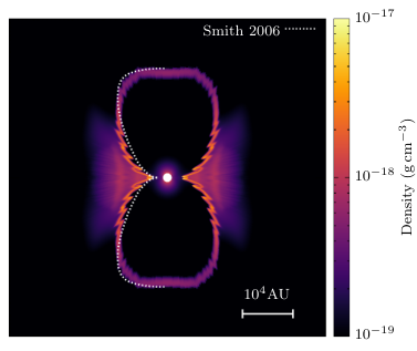
In Figure 5 we show the final snapshot of our fiducial model. There is a clear bipolar thin shell that is very similar to what is seen in Car. The white dotted curve shows the observed Homunculus shape determined by Smith 2006 for comparison. The overall shape of the simulated shell closely resembles that of the observed Homunculus. There are some jagged features along the shell, which is likely due to the “thin-shell instability” or “Vishniac instability” (Vishniac 1983; Kee et al. 2014). However, such features may be due to the strict enforcement of axisymmetry in our simulation and could be smeared out by azimuthal motions in a real 3D case, or more realistic treatments for cooling (Badjin et al. 2016). It also may reproduce the observed mottling of the shells (Smith 2013). Note that the jagged spikes are each resolved with >10 polar grid points and are not reflecting grid-size effects.
To analyse our results more quantitatively, we use the following strategy to identify the shell. The velocity distribution along each radial direction can be divided into three parts; the wind, the shell and the ejecta. The wind has a constant velocity and the ejecta has a linear distribution (), and there is a transitional region in between. We define this transitional region as the shell and calculate the mass-weighted radius and velocity along each latitudinal ray. The total mass in the shell is , which is smaller than the mass estimates from observations (Smith 2006, ;).
The latitudinal distributions are shown in Figure 6. One remarkable feature is that the shell velocity is 10–20 larger than its position divided by time. This means that the shell does not follow a clean homologous expansion and there is a velocity difference between the shell and the ejecta material right above it55 5 This corresponds to in the analysis presented in Appendix B.. Such a difference will alter the apparent ejection date of the shell to slightly (a few decades) after the Great Eruption. The ejection dates inferred from proper motions points to 18471, which is a few years after the peak of the Great Eruption (Smith 2017). Although the discrepancy is much smaller, this is qualitatively in agreement with our model. Any scenario that involves deceleration of Great Eruption ejecta by pre-eruption material will have an apparent ejection date “before” the Great Eruption. The velocity differences decrease towards the equator, implying a latitude-dependent age discrepancy. The width of the shell is 10–15 of the shell radius, but this strongly depends on the treatment of cooling, hence we do not claim this is a robust quantity.
The mass distribution within the shell is also interesting. Although in Figure 5 the density visually looks higher at lower latitudes, there is more mass around the poles when integrated over the width of the shell. The mass distribution is almost constant up to and drops off towards the equator. This is opposite from the mass distribution of the ejecta where there was more mass towards the equator. It also seems to be consistent with the observations that the polar caps are more opaque compared to the side walls (Hillier & Allen 1992; Davidson et al. 2001; Smith 2002, e.g.). However, the mass distribution within the Homunculus walls is sensitive to the details of the eruption and post-eruption winds, and the distribution we show here is not a robust result. The opacity distribution also strongly depends on the dust formation process and we do not attempt to model that in this paper.
There is also a lot of ejecta material () outside the Homunculus in the low-latitude, low-velocity regions that is not yet swept up by the shell. Ultra-violet observations of resonant scattering from Mg ii also show matter outside the Homunculus that spatially coincides with the extended material in our simulations (Smith & Morse 2019), although the current estimated mass () is significantly smaller than what we obtain. The main reason for the mass enhancement in the lower latitudes is due to the oblateness of the pre-eruption envelope shaped by the large amount of angular momentum brought in from the orbit. This is a distinct feature of the merger hypothesis, and is important for the shaping of the Homunculus. However, the ratio between the Homunculus and outer masses can be somewhat tuned by changing the energy injection procedure. For example, weaker energy injection models have less ejecta in the low-latitude regions (Models 3 & 4 in Figure 4). This can still be sculpted into the Homunculus shape by invoking stronger post-eruption winds, and there will be less mass outside the Homunculus since the lower velocity ejecta will be swept up into the shell. Indeed, there are some observational indications that there may be a mass of or more that is already swept up in the equatorial waist of the Homunculus nebula (Morris et al. 2017; Smith et al. 2018a), although with large uncertainties. This could have originally been the lower velocity eruption material that has been swept up by the wind and contributed to the pinching of the Homunculus equator. Therefore, further detailed observational and theoretical investigations of the mass and its distribution of the matter outside the Homunculus may help us understand the structure of the pre-merger envelope, the true nature of the energy deposition and the relative contributions of the eruption and wind for shaping the Homunculus nebula.
In this scenario, the shell should still be slightly accelerating depending on what the wind strength was yr ago. For example in the simulation we show here, the Homunculus expansion speed accelerates by from 2005 to 2020. This could in principle be verified by future detailed observations of the Homunculus.
4 Historical ejections
The Outer Ejecta showing pre-eruption mass loss in multiple precursor eruptions over several hundred years (Kiminki et al. 2016) has been difficult to reconcile with a simple binary merger scenario. A terminal event like a binary merger will in general not produce recursive mass-loss events and therefore requires other mechanisms for pre-eruption mass loss. Smith et al. 2018c proposed that in a triple system, Car’s precursor eruptions that made the Outer Ejecta arose from the interaction of two of the massive stars grazing each others surfaces at high eccentricities, based on studies of unstable orbital dynamics in triples (Perets & Kratter 2012). The eccentricity can be periodically excited through triple body interactions (Perets & Kratter 2012; Shappee & Thompson 2013; Michaely & Perets 2014). In this section we explore the possibility of mass ejections in eccentric orbits and the expected distribution of these ejectiles around the system. We then compare it with various observational properties of the historical ejecta.
There are several observational properties of the outer ejectiles that need to be addressed in any theoretical model for Car’s formation. Based on the ejection dates inferred from the proper motion, there are at least 3 distinct ejection episodes at around the years 1250, 1550 and 1800 A.D. (Kiminki et al. 2016). The velocity range is 300–600 km s-166 6 Note that these are projected velocities so the physical velocities should be larger.. Each ejection episode has a different ejection direction which is not aligned to the Homunculus symmetry axis and, more importantly, is not even bipolar. It rather looks like one-sided sprays of ejecta with some opening angle. Hereafter we will call the historical Outer Ejecta as the “sprays”. Any model for the spray ejection has to self-consistently explain the 300 yr intervals, the 300–600 km s-1 velocities and the disorganised ejection directions.
4.1 Orbital evolution towards merger
Because our scenario assumes that the Homunculus was created through a binary merger, the existence of a current-day companion naturally requires the system to have been a triple prior to the Great Eruption. The possibility of Car being a triple has been raised in the past (Livio & Pringle 1998), and some studies suggest that the triple interactions can cause very close encounters of the stellar components and ultimately trigger a coalescence (Portegies Zwart & van den Heuvel 2016; Smith et al. 2018c). However, the current day orientation of the binary orbit to the Homunculus nebula complicates the problem. The current day orbit of the companion appears to be well aligned with the Homunculus equatorial plane (Gull et al. 2009; Madura et al. 2012). If the Homunculus symmetry axis was determined by the orbit of the merging stars, it would mean that the pre-merger triple system had a small mutual inclination. In normal Kozai-Lidov oscillations the eccentricity reaches high values for systems with large mutual inclination (Kozai 1962; Lidov 1962), so it is expected that the mutual inclination at the time of merger is large. In fact, The Kozai-Lidov mechanism only works for systems with mutual inclinations of ; i.e. the inclination between the merger plane and outer orbit cannot be smaller than this value.77 7 Indeed, Portegies Zwart & van den Heuvel 2016 use mutual inclinations of .. There are some processes where the mutual inclination can be damped after the merger, such as tidal interactions of the inner and outer orbits in the spiral-in phase (Correia et al. 2013) or partial alignment of the spun-up envelope through disk-orbit interaction (Martin et al. 2011). But the time-scales of tidal processes tend to be quite long, so it is unlikely that they reach the observed low inclinations ().
Another puzzling factor is the nature of the companion star itself. The hard X-ray emission at periastron suggests strong colliding wind interactions, implying that the companion wind should have a comparable momentum to that of Car (Corcoran et al. 1995; Corcoran et al. 1997). Hydrodynamical modelling estimates the wind properties of the present-day companion to be yr-1 and km s-1 (Okazaki et al. 2008; Russell et al. 2016; Hamaguchi et al. 2018), which is orders of magnitude stronger and several times faster than the typical wind of a main-sequence star. In fact, it is more consistent with a hydrogen-poor star like Wolf-Rayet (WR) stars (Smith et al. 2018c).
This issue has been discussed by Smith et al. 2018c, and they construct a speculative model that could possibly resolve this. In their model the current companion to Car was initially the most massive star in the triple system which is eventually kicked out to be the tertiary star after losing its hydrogen envelope through mass transfer. In this way the WR-like nature of the current companion and eccentric orbit can naturally be explained.
To investigate this model we consider the evolution of a hierarchical triple system with masses of and for stars A, B and C respectively. We assume that the mutual inclination is initially large (). The system is thus subject to Kozai-Lidov oscillations but the distances at periastron do not get close enough to cause catastrophic interactions. Once star A reaches the end of core hydrogen burning, the star rapidly expands and starts transferring matter to star B. There is a rapid mass-transfer phase until the mass ratio inverts where the donor becomes less massive than the accretor. Part of the mass transferred in this initial short phase may be spilled out from the system because the secondary cannot accrete the transferred matter fast enough. As the mass ratio inverts, the mass transfer becomes stable and thus most of the transferred mass thereafter is expected to be accreted by the secondary. In this situation, mass transfer widens the separation of the inner binary due to angular-momentum conservation. Smith et al. 2018c proposed that this widening of the orbit after mass transfer leads to chaotic orbital evolution and an exchange of partners. Eventually star A loses most of its hydrogen envelope and so develops a strong, fast wind associated with hydrogen-depleted WR stars. This extra mass-loss stage may widen the separation slightly more, further destabilising the system. Unstable systems can undergo chaotic evolution, resulting in various outcomes such as swapping companions, ejecting stars, complete dissociation, or mergers (Eggleton & Kiseleva 1996; Perets & Fabrycky 2009; Perets & Kratter 2012; Antonini & Perets 2012; Antognini et al. 2014; Antognini & Thompson 2016, e.g.). Since star A is hydrogen poor at this stage, the radius is significantly smaller than that of the other two stars. Therefore the larger cross section of the other two stars make them more likely to merge with each other. The hydrogen-poor tertiary star then becomes the present-day secondary star, which may naturally explain the observed strong WR-like wind of the companion (Smith et al. 2018c).
In chaotic situations like this, the closest encounters are not necessarily correlated with the mutual inclination, since the orbits are not well defined. Although it is tempting to give a natural explanation for the alignment of the current day orbit with the Homunculus nebula, here we will just note that in chaotic encounters it is possible to create systems with low mutual inclinations that cannot be achieved in the standard Kozai-Lidov mechanisms.
We carry out 3-body dynamical simulations to study the above scenario. For this we use a few-body integrator that directly integrates the gravitational forces with an 8th-order implicit Runge-Kutta method (Hairer et al. 2000), using the coefficients of Kuntzmann & Butcher (Butcher 1964). With this code we follow the dynamical evolution of a marginally unstable triple system. A triple system becomes dynamically unstable when where are the orbital separations of the inner and outer orbits respectively and is the eccentricity of the outer orbit. is a threshold value that can be estimated by
| (15) |
based on fits to numerical experiments (Valtonen et al. 2008, see also Mardling 2008 for analytic discussions). This fit serves as an upper limit for instability to occur, so most systems become unstable at slightly smaller values of (Valtonen et al. 2008, see Figures 7–11 in). We set the initial condition of our triple system assuming that the system recently reached low values due to mass transfer/loss.
Figure 7 displays an example of the time evolution of distances between bodies in an unstable triple system. The initial parameters are given in the caption, which corresponds to . The system is relatively stable for the first yr, where the inner eccentricity oscillates between 0 and 0.7 due to the Kozai-Lidov mechanism. After yr, the quasi-secular regime commences and causes modulations in the minimum distances (maximum eccentricities) reached in the Kozai-Lidov cycles. It is not clear what sets the time-scales of these modulations, but it should be pointed out that the intervals between the minimum distance peaks are yr for this case, not far off from the yr intervals of the observed sprays of Car. The minimum distances reached in this chaotic phase is – (–0.89), which is comparable to the stellar radius of a main-sequence star. Also, the minimum distance peaks are slightly deeper at later times. It may be possible that star A plunges into the envelope of star B several times, but the density in the radiative envelopes of massive stars are extremely low and therefore the drag force that acts on a WR star companion is minute unless it plunges even deeper, such as down to the surface of the convective core (See Appendix C for discussions on how deep the WR needs to plunge in). At about yr, the system becomes even more chaotic and multiple swaps of companions occur at around yr. The minimum distance between stars B and C reach as low as . Unlike star A, star C has a large radiative envelope, so the interaction with star B’s envelope can be more violent than interacting with a small hydrogen-poor star. Therefore the minimum distance in this case may be small enough to trigger a catastrophic merger. The time-scale of the system reaching this disruptive point is of comparable scale to analytic estimates derived from simple random walk models (Mushkin & Katz 2020, yr;). Figure 8 illustrates the complexity of the orbits in the last 6 months leading to the onset of merger. If we assume that stars B and C started merging at this point ( yr), the inclination between the Homunculus nebula and the current day orbit will be or slightly smaller due to post-merger damping effects. Considering that the 3D orientation of the current day orbit still contains uncertainties (Madura et al. 2012), this small mutual inclination may already be small enough. The post-merger eccentricity is , which is also consistent with current estimates of Car’s orbit (Kashi & Soker 2007, e.g.).


As a plausibility check, we conducted the same 3-body calculation but with instead of . This corresponds to a slightly higher value (), and found that this system was stable for yr. This means that the system was stable before the widening phase so that the chaotic interactions do not occur in the earlier stages of its evolution. The instability only started after star A evolved off the main sequence, initiating mass transfer and widening the inner orbit. This is also consistent with the 3--4 Myr age of the Tr 16 cluster88 8 Recent parallax measurements suggest that Car is unrelated to Tr 16 (Davidson et al. 2018). (Walborn 2012).
These numerical simulations confirm that the model proposed by Smith et al. 2018c is quantitatively plausible. It remains to be determined, though, how common or rare such a scenario may be. The results we present here are only for one particular set of initial conditions as a proof of concept. Small deviations in the initial conditions (e.g. masses, inclination, orbital phase) can result in qualitatively different outcomes due to the chaotic nature of the system. We have carried out 1000 simulations of the same triple system but with variations in the initial orbital phase of the inner binary. Out of our runs, 26% of them resulted in a stellar merger within 3000 yr. Only 2–3% experienced companion swaps within the same time frame. A wider statistical analysis is required to quantify whether the modulating Kozai-Lidov cycles, swapping of companion and a final merger is a preferred outcome or a rare case. We will postpone such analyses to future work.
4.2 Mass ejection from close periastron encounters
When the eccentricity reaches extremely high values, the periastron distance can become comparable to the stellar radius and can sometimes even graze the surface of each star. These close interactions will pull off and eject material in confined directions (Smith et al. 2018c). In more extreme cases, stars can plunge deep into the envelope where the frictional force can rapidly take away orbital energy and trigger a fatal merger (Perets & Kratter 2012, e.g.).
To explore the outcome of grazing encounters, we conduct a simple experimental calculation of how surface material on a star reacts to the gravitational force of an approaching secondary star in an eccentric orbit. For this we use the same few-body integrator as above. To represent surface material of a star, we introduce an artificial “glue” force around the primary star that prevents particles from falling to the centre but instead keeps it rotating around the star at a constant spin velocity at a constant radius. This artificial force is smoothly switched off once the particle is lifted off the surface of the star. We randomly place test particles on the surface of the primary star and let it rotate at either periastron orbital angular velocity or critical rotation, whichever is smaller. It is assumed that the star has been tidally spun up through multiple encounters, or is rapidly rotating due to the preceding mass accretion. 50 particles are placed on the star and we follow its orbital evolution through 500 orbits of the secondary. Whenever a test particle reaches a distance of more than 10 times the semimajor axis away from the centre of mass, we record the direction and velocity of the ejection and put it back on a random position of the surface of the star. This procedure is equivalent to calculating a single encounter with more surface particles, but maximises the efficiency of the few-body integrator. We also remove particles whenever it gets closer than to the secondary star, assuming it is accreted or deflected by winds.
Figure 9 shows that test-particle trajectories behave in roughly three different ways. Some are simply lifted off the surface slightly and placed on eccentric bound orbits around the primary. A second group wrap around the trajectory of the secondary star, indicating mass transfer. But a third group reaches out of the panel, becoming unbound from the system and so forming spray ejecta. The sky map of spray directions is shown in Figure 10. Velocities are calculated by asigning a scale of and . Most spray particles are confined within from the orbital plane. There is a clear cluster of spray particles on the left which are the particles ejected downwards in Figure 9. Because these particles are already weakly bound to the star due to the spin, the gravitational lift at periastron sends them on hyperbolic orbits around the primary and out of the system. There is another weak cluster on the right which corresponds to the particles shooting out to the left in Figure 9 and are more spread out. These particles are flung away from the close vicinity of the secondary star.
We then split up the sky into bins and calculate the average spray velocity in each direction. Figure 11 shows the velocity in each bin overplotted on a histogram of the number of particles ejected in each direction. It is clear that the majority of the ejected particles are clustered in one direction with an opening angle of . The sprays have velocities in the range 100–500 km s-1 while an extremely small number of particles reach up to km s-1. The maximum velocity of the bulk ejecta ( km s-1) is roughly determined by the asymptotic velocity of a hyperbolic orbit which was launched at the surface of the primary and had an initial angular velocity equivalent to the orbital angular velocity at periastron
| (16) |
The velocity roughly follows a linear distribution, with maximum velocity at and declining up to 0.


To explore how the sprays depend on the orbital parameters, we have carried out an additional set of simulations. We find that when the semimajor axis is fixed, just a slight decrease in eccentricity can significantly affect the amount of spray ejecta. Figure 12 shows the particle trajectories for the case where . There are a few particles being transferred to the secondary but none of them are ejected from the system. For eccentricities of we found that there are not even any transferred particles. A comparison between the three different eccentricities can be seen in the movie available online (Movie 4). It seems that there is a well-defined threshold above which sprays can happen. This can be understood by comparing the orbital angular velocity at periastron
| (17) |
and the critical spin angular velocity
| (18) |
When , the secondary star exhibits a spin-up torque to the primary. If the surface is already rotating at critical, these particles are marginally bound so the small acceleration can make them unbound, resulting in spray ejection. In other cases, the secondary exhibits a spin-down torque, so the surface particles never become unbound. Figure 13 shows when the two angular velocities cross over. In a hierarchical triple system, the Kozai-Lidov mechanism causes the inner orbit to librate and change eccentricity while the semimajor axis is fixed. Note that at any given semimajor axis, there exists a critical eccentricity above which spray ejection can occur. For the examples shown in Figures 9 & 12, the semimajor axis is fixed to and the transition between spraying and non-spraying cases can be well explained by this critical eccentricity. This is of course strongly tied to the assumption that the primary is already rapidly spinning. This is probably not a bad assumption since the primary star in this case is the mass accretor in the previous evolution. In our scenario, the mass-transfer stage is not too long before the spray ejection stage, so any spin-down mechanism would not have actively spun down the star yet. Also, the tidal torques from the orbit at periastron will keep it rapidly rotating.

The above simulation indicates that eccentric close encounters can send out material in confined directions. There is a preferred direction perpendicular to the eccentricity vector, with an opening angle of . Along with the ejection velocity (100–500 km s-1), these periastron sprays are in good agreement with the observed sprays (Kiminki et al. 2016). Multiple periastron passages will send out several sprays, which will interact with each other. Self-interaction shocks could quickly cool the material, and make them clumpy. We have only tracked the motion of test particles, so we are not able to give quantitative estimates on the amount of ejected mass. There is very little mass located in the surface layers. For example, there is only 0.1 in the outer 1/3 of the stellar radius for a 50 main sequence star. Therefore the total amount of ejected mass through these close encounters should be considerably less https://www.overleaf.com/project/5f445c31ef47a700014dedf1than 0.1. It should also be noted that we have only considered purely gravitational effects in this simple calculation. In reality the stars could graze each others surface, and non-gravitational effects such as shocks and radiation would influence the mass ejection from the system too. Further research is required to investigate how much the other interactions can contribute to the spray ejecta and whether they have similar ejection directions, and how much mass can be ejected.
Because the sprays are produced from the surface material of the mass accretor (star B), it is possible that they have chemical peculiarities. Indeed, the observed spray material are known to be nitrogen rich (Davidson et al. 1982), with a decreasing amount of N enrichment farther from the star (Smith & Morse 2004). It will be interesting to estimate the precise chemical composition of the spray ejecta in future studies.
4.3 Spatial distribution of sprays
By combining our simulation results in the previous sections, we can predict the spatial distribution of spray ejecta around the Homunculus. For simplicity, we do not carry out a large grid of spray simulations but instead fit a simple functional form to the velocity distribution of spray particles
| (19) |
where is computed from Eq. (16). The forefactor simply accounts for the linear distribution in . Although not a perfect fit to the spray simulation results, this roughly gives the velocity scaling and angular distribution (pink and red dots) in Figure 11.
We next apply this formula to the sample triple system in section 4.1. We assume that stars B and C started merging when the distance between the two stars first reached down to ( yr). At every periastron passage before that, where , we assume that a spray was ejected along the orbital plane with a velocity distribution following Eq. (19). By assuming the spray ejecta follow ballistic trajectories, we can calculate the positions of ejecta at arbitrary times. In Figure 14 we show the position and velocity vectors of spray ejectiles 176 yr after the Great Eruption. Here we have assumed that the Great Eruption occurred 30 yr after the onset of the merger. To mimick the clumpiness of the sprays, we have only selected 3–4 random directions within the opening angle for each periastron passage. The particles are colour coded by the apparent ejection date assuming the Great Eruption occurred in 1844. A Homunculus model is placed at the centre, with the symmetry axis taken in the direction of the orbital angular momentum vector of the merging binary. There are 5–6 distinct ejection episodes in this figure, corresponding to the eccentricity peaks seen in Figure 7. Each ejection is one-sided and points in a different direction. None of the ejections are aligned with the symmetry axis of the Homunculus or with the equatorial plane. This highly asymmetric and randomly directed nature is remarkably consistent with the observed Outer Ejecta (Kiminki et al. 2016, right panel;). The velocities also show an increasing trend towards more recently ejected sprays. This is because Eq. (16) gives higher velocities for higher eccentricities, and the eccentricity increases over time in this system (Figure 7). The closer-in red vectors could correspond to the ghost shell or outer shell observed in H (Mehner et al. 2016). The background image is produced by integrating along each line of sight, representing the H emission.

We have not considered any overtaking in this calculation. In reality the faster later sprays that overtake slower earlier sprays can wipe out their traces, reducing the number of sprays observed today and possibly enhance the clumpiness. Also, we have made an arbitrary choice for the delay time between the onset of merger and the Great Eruption. We can, however, constrain the delay time to some degrewe. Kiminki et al. 2016 suggest that the prior mass ejections occurred in 1250, 1550 and early 1800s. If the 1800s outburst was due to a close encounter, the merger should have happened after 1800 but before the Great Eruption in 1844, meaning that the spiral-in process took less than 44 years. We have also suggested that the precursor eruptions in 1838 and 1843 were due to interactions between the binary companion and the bloated envelope during the spiral-in phase (Figure 1, Panel 3-2). This indicates that the common-envelope phase started before 1838, placing a lower limit of yr for the spiral-in time-scale. So the merger delay time can be narrowed down to 6–50 yr, which will not significantly affect the results shown in Figure 14.
The example demonstrated in this section is not the only possible path. For example, the companion swap could have happened much earlier and the sprays could have occurred through interactions between stars B and C. There could have been a triple common-envelope phase where the envelope of the tertiary expands to engulf the inner binary (Glanz & Perets 2021). By the time the envelope is shedded, the tertiary becomes a hydrogen-poor star and the inner and outer orbits can both shrink to an unstable configuration. The sprays and merger can occur shortly after. Our basic picture does not change in any case. The main point is that the system starts off as a hierarchical triple system but becomes unstable once one of the stars evolves off the main sequence. Chaotic Kozai-Lidov cycles enables close encounters of stars and sends out spray ejecta. The unstable orbit eventually triggers a merger which causes the Great Eruption and shapes the bipolar Homunculus nebula.
The one-sided ejections, random orientations and yr intervals of the sprays are all difficult to explain in most of the previously proposed models. Whereas in the triple evolution scenario proposed by Smith et al. 2018c that we investigate in more detail here, all these features are naturally expected. From the above experiments, we now confirm that the historical eruptions and Outer Ejecta are no longer counter-arguments to the merger scenario but may instead be supporting evidence for the model.
5 Post-merger evolution
Following the merger, we have assumed that the energy from the merger that was not carried away in the eruption is radiated as enhanced luminosity, observed initially to range up to a value (Frew 2004; Smith & Frew 2011). This is well above the Eddington luminosity, and so can drive a mass loss up to the energy limit (Owocki et al. 2017), which here can be more than two orders of magnitude higher than even the very strong current-day mass loss of yr-1. The strong wind should cease once all the excess energy is radiated away and the star regains thermal equilibrium. Although the post-merger star could have a non-standard chemical profile due to the strong mixing during the merger, the star should continue its evolution as a normal single star of the mass of the merger product (Schneider et al. 2020). If any of the merging stars was depleted in hydrogen in the core, it could experience a prolonged phase of hydrogen shell burning, spending more time as a blue supergiant than that of a star of the same mass (Glebbeek et al. 2013).
Stars in this mass range () are expected to have very strong winds and experience luminous blue variable activity, so the mass-loss rate should be relatively high even without the enhanced luminosity due to the merger. Therefore Car can lose nearly a half or more of its own mass during its lifetime. The final fate of these stars are rather uncertain. One possible outcome is that it simply collapses into a black hole. In this case, most of the mass in the star will be retained and could form a several black hole. The kick velocity imparted to black holes are expected to be quite small, so the binary would not disrupt. Because the likely outcome of the companion star ( Car B) is also black hole formation, the system could become a very eccentric binary black hole. The other possible fate of the merger product is a pulsational or non-pulsational pair-instability supernova. In the former case, it will experience several large pulsations and end up as a normal core-collapse or failed supernova. In the latter case the whole star will be expelled in the explosion and will not leave any remnant. However, this may be unlikely at solar metallicities () due to the large mass loss that hinders the establishment of a massive enough core (Langer et al. 2007).
We also note that, if the merger takes place with the original primary (i.e. if star A is not swapped out of the inner orbit), which is already a post-main-sequence star at the time of the merger, the subsequent evolution of the merger product could be quite different (Justham et al. 2014, see also Vanbeveren et al. 2013; Vigna-Gómez et al. 2019). Specifically, it is likely to spend most of its helium core-burning phase as a blue supergiant and become a luminous blue variable (of the S Doradus type) shortly before it explodes in a supernova (Justham et al. 2014).
6 Discussion
In our eruption simulation we have not taken into account any other possible sources of energy other than the gravitational and orbital energy of the core binary. Other processes may tap in extra sources of energy such as explosive nuclear burning when fresh fuel is dragged in to the higher temperature regions (Ivanova et al. 2002; Ivanova & Podsiadlowski 2002). However, this would only be significant if one of the merging stars have depleted hydrogen in their core, which is not the case for our fiducial model laid out in Figure 1. Magnetic fields could also play an important role (Schneider et al. 2019). We have also only used a single model for our combined mass () but the total mass could have been larger. In that case the core masses would have been larger too, implying that there was more orbital energy in the core binary. All these effects could tap in more energy to the eruption, leading to more violent explosions and therefore more ejecta mass. These processes may be fundamentally important if the true Homunculus mass is much greater than the inferred lower limits (Smith et al. 2003a; Morris et al. 2017, 10–45;).
The highest velocities achieved in our eruption simulations reached up to 10,000 km s-1 although the mass in that high velocity matter is tiny. Such velocities are in fact observed in light echoes (Smith et al. 2018b). It should be noted that, in our simulation, the equatorial shock breakout has slightly faster velocities than the polar shock breakout. This is likely caused by the way we set the background density. Because we set a slow wind as a background, the density is higher at smaller radii. Therefore the density contrast between the stellar surface and outside is smaller around the poles, so the immediate shock breakout velocity is slightly slower. Because the mass in the fast components are small, it will easily be decelerated as it runs into slower pre-eruption wind material that was flowing at 150–200 km s-1 (Smith et al. 2018c). The degree of deceleration will depend on the mass-loss rate of the pre-eruption wind. At some point this fast Outer Ejecta material will catch up and collide with even denser pre-eruption ejecta such as the spray material from the historical ejections or L2 outflow material from the mass-transfer phase. It has been proposed that this collision between extremely fast ejecta from the Great Eruption and slower pre-eruption ejecta is the origin of the observed soft X-ray shell around Carinae (Smith & Morse 2004; Smith 2008). X-rays are in fact observed from the outer regions and the estimated shock velocities are 700–800 km s-1 (Seward et al. 2001; Weis et al. 2004). This is roughly consistent with the relative velocity between spray ejecta velocities and the eruption ejecta velocity inferred from the location of the X-rays99 9 The eruption ejecta velocity is simply where is the distance from the star and is the time since the Great Eruption..
This scenario does not naturally explain the origin of the lesser eruptions that occurred after the Great Eruption. The lesser eruption around 1890 is considered to have created the Little Homunculus that lies inside the Homunculus nebula itself (Ishibashi et al. 2003; Smith 2005). Its inferred apparent ejection date is around 1910–1930, meaning that if it was really ejected in the 1890s, the Little Homunculus is likely being swept up and accelerated in a similar way to the main Homunculus in our scenario (Smith 2005). What caused the 1890s eruption is still an open question. Some studies claim that the lesser eruptions were triggered by interactions with the secondary at periastron (Kashi & Soker 2010). However, their model requires extremely high masses for both the primary and secondary stars (, ), which are factors of 2–3 larger than the observationally inferred values.
Some other important visible features of the Outer Ejecta are the “NN jet”, S condensation and the equatorial “skirt” (Walborn 1976; Meaburn et al. 1996; Morse et al. 1998; Kiminki et al. 2016; Mehner et al. 2016). These structures have slightly older apparent ages, but could be consistent with being ejected in the Great Eruption if it was decelerated later on (Morse et al. 2001; Kiminki et al. 2016; Smith 2017). Moreover, the NN jet and the S condensation seem to be aligned with the direction of some non-axisymmetric features of the Homunculus known as “protrusions” (Steffen et al. 2014). The protrusions are located roughly 110 apart, where the centre points in the direction of the opening in the CO torus observed by ALMA (Smith et al. 2018a). Together with the fact that the apocentre of the current-day binary orbit points towards the gap in the torus (Madura et al. 2012), Smith et al. 2018c proposed that all these structures were possibly shaped by the binary companion plunging through the bloated common envelope or circumstellar torus. In Phase 3-2 of our scenario (see Fig. 1), the companion could have plunged through the envelope multiple times, punching a hole in it. The momentum of the companion wind is relatively small, so it could only drill small tunnels. As pointed out by Smith et al. 2018b, the later Great Eruption will be channeled through the holes, squirting out a narrow feature like the NN jet. However, it is not clear whether the envelope distortions could have been sustained until the Great Eruption since the rotational period of the envelope is relatively short ( yr) and the rotation could have quickly smeared out any small distortions.
7 Conclusion
We have performed a suite of numerical simulations to investigate the merger-in-a-triple scenario for the origin of Carinae and its multiple eruptions similar to the model proposed by Smith et al. 2018c (Fitzpatrick 2012, see also). Our study confirms that this scenario gives a plausible explanation for the Great Eruption of Carinae. In addition, our simulations suggest that the strong bipolar wind from the merger product played a critical role in sweeping up and shaping the bipolar Homunculus after the eruption.
We first carry out 2.5D hydrodynamical simulations of the outflow from an explosive stellar merger event. The ejecta follow a homologous expansion, and are distributed in a rather spherical manner. We then inject a strong bipolar wind following a standard gravity-darkening law to see how the ejecta get swept up into a thin shell. We find that we can reproduce the shape of the Homunculus nebula fairly well, although with some remaining questions about the latitudinal and radial mass distribution.
Because Car is a binary system today, the system must have started off as a triple system if Car is indeed a merger product. We expect that the system was unstable in the past and could have experienced swaps of companions and close encounters of stars which eventually triggered the merger. We demonstrate through 3-body dynamical simulations that an unstable triple system can induce companion swaps and close encounters under the right conditions. We also carry out N-body simulations of how the surface material on a star reacts to the periastron passage in a highly eccentric orbit. When the eccentricity exceeds a certain threshold, the surface particles can be ejected in one direction with a opening angle along the orbital plane. By combining the triple dynamical evolution and the mass ejection from single close encounters, we estimate how the ejected matter should be distributed around the Homunculus. The one-sided nature of each ejection, the seemingly random ejection directions and yr intervals all agree well with the observed distribution of the Outer Ejecta (Kiminki et al. 2016).
Both our hydrodynamical simulations of mass outflow from the merger and dynamical simulations of the pre-merger evolution reproduce many of the key features of Car’s observed nebula, strongly supporting the merger-in-a-triple scenario (Smith et al. 2018c). We can therefore use Car as a prototype to deepen our understanding of stellar mergers in general. Massive stellar mergers can be responsible for a diverse range of phenomena, such as luminous blue variables and supernova impostors (Smith et al. 2011), peculiar supernovae like SN1987A (Podsiadlowski et al. 1990), magnetic stars (Schneider et al. 2019), or creating interaction-powered supernova progenitors (Justham et al. 2014; Smith & Arnett 2014). The B[e] star binary R4 in the Small Magellanic Cloud is a particularly similar case that has been claimed to be the outcome of a stellar merger in a triple system (Pasquali et al. 2000; Wu et al. 2020). Given the relatively high fraction of massive stars in triple systems (Raghavan et al. 2010; Moe & Di Stefano 2017), it may mean that Car-like systems are not uncommon. The rich observational data for Car can therefore not only help us decipher its own history, but also the origin of many other important astrophysical phenomena.
Acknowledgements
The authors thank the anonymous referee for the constructive comments that improved the content. The authors thank Lorne Nelson for sharing computational facilities. The computations were partially carried out on facilities managed by Calcul Québec and Compute Canada. RH was supported by the JSPS Overseas Research Fellowship No.29-514 and a grant from the Hayakawa Satio Fund awarded by the Astronomical Society of Japan. The work has also been supported by a Humboldt Research Award to PhP. at the University of Bonn. SPO acknowledges a Royal Society International Exchange grant that supported his visit to the University of Oxford in the early stages of this project. FRNS has received funding from the European Research Council (ERC) under the European Union’s Horizon 2020 research and innovation programme (Grant agreement No. 945806). NS received support from National Science Foundation (NSF) grant AST-1515559, and from NASA grants GO-14586, GO-15289, GO-15596, and GO-15823 from the Space Telescope Science Institute, which is operated by the Association of Universities for Research in Astronomy, Inc. under NASA contract NAS 5-26555.
Data Availability
The data underlying this article will be shared on reasonable request to the corresponding author.
References
- Akashi & Kashi (2020) Akashi M., Kashi A., 2020, MNRAS, 494, 3186
- Akashi & Soker (2016) Akashi M., Soker N., 2016, MNRAS, 462, 206
- Antognini & Thompson (2016) Antognini J. M. O., Thompson T. A., 2016, MNRAS, 456, 4219
- Antognini et al. (2014) Antognini J. M., Shappee B. J., Thompson T. A., Amaro-Seoane P., 2014, MNRAS, 439, 1079
- Antonini & Perets (2012) Antonini F., Perets H. B., 2012, ApJ, 757, 27
- Badjin et al. (2016) Badjin D. A., Glazyrin S. I., Manukovskiy K. V., Blinnikov S. I., 2016, MNRAS, 459, 2188
- Barkat et al. (1967) Barkat Z., Rakavy G., Sack N., 1967, Phys. Rev. Lett., 18, 379
- Begelman (2001) Begelman M. C., 2001, ApJ, 551, 897
- Bustamante et al. (2019) Bustamante J., Madura T., Russell C., Gull T., 2019, in American Astronomical Society Meeting Abstracts #233. p. 348.21
- Butcher (1964) Butcher J. C., 1964, Mathematics of Computation, 18, 50
- Chevalier & Fransson (1992) Chevalier R. A., Fransson C., 1992, ApJ, 395, 540
- Clementel et al. (2014) Clementel N., Madura T. I., Kruip C. J. H., Icke V., Gull T. R., 2014, MNRAS, 443, 2475
- Corcoran et al. (1995) Corcoran M. F., Rawley G. L., Swank J. H., Petre R., 1995, ApJ, 445, L121
- Corcoran et al. (1997) Corcoran M. F., Ishibashi K., Swank J. H., Davidson K., Petre R., Schmitt J. H. M. M., 1997, Nature, 390, 587
- Correia et al. (2013) Correia A. C. M., Boué G., Laskar J., Morais M. H. M., 2013, A&A, 553, A39
- Cranmer & Owocki (1995) Cranmer S. R., Owocki S. P., 1995, ApJ, 440, 308
- Currie et al. (2002) Currie D. G., Dorland B. N., Kaufer A., 2002, A&A, 389, L65
- Damineli (1996) Damineli A., 1996, ApJ, 460, L49
- Damineli et al. (1997) Damineli A., Conti P. S., Lopes D. F., 1997, New Astron., 2, 107
- Damineli et al. (1998) Damineli A., Stahl O., Kaufer A., Wolf B., Quast G., Lopes D. F., 1998, A&AS, 133, 299
- Damineli et al. (2000) Damineli A., Kaufer A., Wolf B., Stahl O., Lopes D. F., de Araújo F. X., 2000, ApJ, 528, L101
- Davidson et al. (1982) Davidson K., Walborn N. R., Gull T. R., 1982, The Astrophysical Journal, 254, L47
- Davidson et al. (2001) Davidson K., Smith N., Gull T. R., Ishibashi K., Hillier D. J., 2001, AJ, 121, 1569
- Davidson et al. (2018) Davidson K., Helmel G., Humphreys R. M., 2018, Research Notes of the American Astronomical Society, 2, 133
- Duschl et al. (1995) Duschl W. J., Hofmann K. H., Rigaut F., Weigelt G., 1995, in Niemela V., Morrell N., Feinstein A., eds, Revista Mexicana de Astronomia y Astrofisica Conference Series Vol. 2, Revista Mexicana de Astronomia y Astrofisica Conference Series. p. 17 (arXiv:astro-ph/9410090)
- Dwarkadas & Balick (1998) Dwarkadas V. V., Balick B., 1998, AJ, 116, 829
- Eggleton & Kiseleva (1996) Eggleton P. P., Kiseleva L. G., 1996, in Wijers R. A. M. J., Davies M. B., Tout C. A., eds, NATO Advanced Study Institute (ASI) Series C Vol. 477, Evolutionary Processes in Binary Stars. p. 345 (arXiv:astro-ph/9510110)
- Fernández-Lajús et al. (2009) Fernández-Lajús E., et al., 2009, A&A, 493, 1093
- Fitzpatrick (2012) Fitzpatrick B., 2012, PhD thesis
- Frank et al. (1995) Frank A., Balick B., Davidson K., 1995, ApJ, 441, L77
- Frank et al. (1998) Frank A., Ryu D., Davidson K., 1998, ApJ, 500, 291
- Frew (2004) Frew D. J., 2004, Journal of Astronomical Data, 10, 6
- Fujibayashi et al. (2018) Fujibayashi S., Kiuchi K., Nishimura N., Sekiguchi Y., Shibata M., 2018, ApJ, 860, 64
- Gallagher (1989) Gallagher J. S., 1989, in Davidson K., Moffat A. F. J., Lamers H. J. G. L. M., eds, Astrophysics and Space Science Library Vol. 157, IAU Colloq. 113: Physics of Luminous Blue Variables. p. 185, doi:10.1007/978-94-009-1031-7_22
- Garcia-Segura et al. (1997) Garcia-Segura G., Langer N., Mac Low M. M., 1997, LBV Outbursts: The Effects of Rotation. p. 332
- Gaviola (1950) Gaviola E., 1950, ApJ, 111, 408
- Ginat et al. (2020) Ginat Y. B., Glanz H., Perets H. B., Grishin E., Desjacques V., 2020, MNRAS, 493, 4861
- Glanz & Perets (2018) Glanz H., Perets H. B., 2018, MNRAS, 478, L12
- Glanz & Perets (2021) Glanz H., Perets H. B., 2021, MNRAS, 500, 1921
- Glebbeek et al. (2013) Glebbeek E., Gaburov E., Portegies Zwart S., Pols O. R., 2013, MNRAS, 434, 3497
- Gnat & Sternberg (2007) Gnat O., Sternberg A., 2007, ApJS, 168, 213
- González (2018) González R. F., 2018, A&A, 609, A69
- González et al. (2004a) González R. F., de Gouveia Dal Pino E. M., Raga A. C., Velazquez P. F., 2004a, ApJ, 600, L59
- González et al. (2004b) González R. F., de Gouveia Dal Pino E. M., Raga A. C., Velázquez P. F., 2004b, ApJ, 616, 976
- González et al. (2010) González R. F., Villa A. M., Gómez G. C., de Gouveia Dal Pino E. M., Raga A. C., Cantó J., Velázquez P. F., de La Fuente E., 2010, MNRAS, 402, 1141
- Grant et al. (2020) Grant D., Blundell K., Matthews J., 2020, MNRAS, 494, 17
- Groh et al. (2012) Groh J. H., Madura T. I., Hillier D. J., Kruip C. J. H., Weigelt G., 2012, ApJ, 759, L2
- Gull et al. (2009) Gull T. R., et al., 2009, MNRAS, 396, 1308
- Gull et al. (2011) Gull T. R., Madura T. I., Groh J. H., Corcoran M. F., 2011, ApJ, 743, L3
- Gustafson (1998) Gustafson K., 1998, Contemporary Mathematics, 218, 432
- Hackwell et al. (1986) Hackwell J. A., Gehrz R. D., Grasdalen G. L., 1986, ApJ, 311, 380
- Hairer et al. (2000) Hairer E., Nørsett S., Wanner G., 2000, Solving Ordinary Differential Equations I Nonstiff problems, second edn. Springer, Berlin
- Hamaguchi et al. (2018) Hamaguchi K., et al., 2018, Nature Astronomy, 2, 731
- Harpaz & Soker (2009) Harpaz A., Soker N., 2009, New Astron., 14, 539
- Hillier & Allen (1992) Hillier D. J., Allen D. A., 1992, A&A, 262, 153
- Hillier et al. (2006) Hillier D. J., et al., 2006, ApJ, 642, 1098
- Hirai et al. (2016) Hirai R., Nagakura H., Okawa H., Fujisawa K., 2016, Phys. Rev. D, 93, 083006
- Hirai et al. (2018) Hirai R., Podsiadlowski Ph., Yamada S., 2018, ApJ, 864, 119
- Iaconi et al. (2017) Iaconi R., Reichardt T., Staff J., De Marco O., Passy J.-C., Price D., Wurster J., Herwig F., 2017, MNRAS, 464, 4028
- Iben (1999) Iben I. J., 1999, in Morse J. A., Humphreys R. M., Damineli A., eds, Astronomical Society of the Pacific Conference Series Vol. 179, Eta Carinae at The Millennium. p. 367
- Ishibashi et al. (1999) Ishibashi K., Corcoran M. F., Davidson K., Swank J. H., Petre R., Drake S. A., Damineli A., White S., 1999, ApJ, 524, 983
- Ishibashi et al. (2003) Ishibashi K., et al., 2003, AJ, 125, 3222
- Ito & Ohtsuka (2019) Ito T., Ohtsuka K., 2019, Monographs on Environment, Earth and Planets, 7, 1
- Ivanova & Podsiadlowski (2002) Ivanova N., Podsiadlowski Ph., 2002, Ap&SS, 281, 191
- Ivanova et al. (2002) Ivanova N., Podsiadlowski Ph., Spruit H., 2002, MNRAS, 334, 819
- Ji et al. (2013) Ji S., et al., 2013, ApJ, 773, 136
- Justham et al. (2014) Justham S., Podsiadlowski Ph., Vink J. S., 2014, ApJ, 796, 121
- Kashi & Soker (2007) Kashi A., Soker N., 2007, New Astron., 12, 590
- Kashi & Soker (2010) Kashi A., Soker N., 2010, ApJ, 723, 602
- Kashi & Soker (2016) Kashi A., Soker N., 2016, ApJ, 825, 105
- Kee et al. (2014) Kee N. D., Owocki S., ud-Doula A., 2014, MNRAS, 438, 3557
- Kiminki et al. (2016) Kiminki M. M., Reiter M., Smith N., 2016, MNRAS, 463, 845
- Kozai (1962) Kozai Y., 1962, AJ, 67, 591
- Langer et al. (1999) Langer N., García-Segura G., Mac Low M.-M., 1999, ApJ, 520, L49
- Langer et al. (2007) Langer N., Norman C. A., de Koter A., Vink J. S., Cantiello M., Yoon S. C., 2007, A&A, 475, L19
- Leung et al. (2019) Leung S.-C., Nomoto K., Blinnikov S., 2019, ApJ, 887, 72
- Lidov (1962) Lidov M. L., 1962, Planet. Space Sci., 9, 719
- Livio & Pringle (1998) Livio M., Pringle J. E., 1998, MNRAS, 295, L59
- MacLeod et al. (2018) MacLeod M., Ostriker E. C., Stone J. M., 2018, ApJ, 868, 136
- Madura et al. (2012) Madura T. I., Gull T. R., Owocki S. P., Groh J. H., Okazaki A. T., Russell C. M. P., 2012, MNRAS, 420, 2064
- Madura et al. (2013) Madura T. I., et al., 2013, MNRAS, 436, 3820
- Maeder & Meynet (2000) Maeder A., Meynet G., 2000, A&A, 361, 159
- Mardling (2008) Mardling R. A., 2008, Resonance, Chaos and Stability: The Three-Body Problem in Astrophysics. p. 59, doi:10.1007/978-1-4020-8431-7_3
- Martin et al. (2011) Martin R. G., Pringle J. E., Tout C. A., Lubow S. H., 2011, MNRAS, 416, 2827
- Meaburn et al. (1996) Meaburn J., Boumis P., Walsh J. R., Steffen W., Holloway A. J., Williams R. J. R., Bryce M., 1996, MNRAS, 282, 1313
- Mehner et al. (2010) Mehner A., Davidson K., Humphreys R. M., Martin J. C., Ishibashi K., Ferland G. J., Walborn N. R., 2010, ApJ, 717, L22
- Mehner et al. (2016) Mehner A., et al., 2016, A&A, 595, A120
- Michaely & Perets (2014) Michaely E., Perets H. B., 2014, ApJ, 794, 122
- Miyoshi & Kusano (2005) Miyoshi T., Kusano K., 2005, Journal of Computational Physics, 208, 315
- Moe & Di Stefano (2017) Moe M., Di Stefano R., 2017, ApJS, 230, 15
- Morris & Podsiadlowski (2006) Morris T., Podsiadlowski Ph., 2006, MNRAS, 365, 2
- Morris et al. (2017) Morris P. W., Gull T. R., Hillier D. J., Barlow M. J., Royer P., Nielsen K., Black J., Swinyard B., 2017, ApJ, 842, 79
- Morse et al. (1998) Morse J. A., Davidson K., Bally J., Ebbets D., Balick B., Frank A., 1998, AJ, 116, 2443
- Morse et al. (2001) Morse J. A., Kellogg J. R., Bally J., Davidson K., Balick B., Ebbets D., 2001, ApJ, 548, L207
- Mushkin & Katz (2020) Mushkin J., Katz B., 2020, MNRAS, 498, 665
- Nielsen et al. (2007) Nielsen K. E., Corcoran M. F., Gull T. R., Hillier D. J., Hamaguchi K., Ivarsson S., Lindler D. J., 2007, ApJ, 660, 669
- Ohlmann et al. (2016) Ohlmann S. T., Röpke F. K., Pakmor R., Springel V., 2016, ApJ, 816, L9
- Okazaki et al. (2008) Okazaki A. T., Owocki S. P., Russell C. M. P., Corcoran M. F., 2008, MNRAS, 388, L39
- Ostriker (1999) Ostriker E. C., 1999, ApJ, 513, 252
- Ostriker & Gunn (1971) Ostriker J. P., Gunn J. E., 1971, ApJ, 164, L95
- Owocki (2005) Owocki S., 2005, in Humphreys R., Stanek K., eds, Astronomical Society of the Pacific Conference Series Vol. 332, The Fate of the Most Massive Stars. p. 171
- Owocki & Gayley (1997) Owocki S. P., Gayley K. G., 1997, in Nota A., Lamers H., eds, Astronomical Society of the Pacific Conference Series Vol. 120, Luminous Blue Variables: Massive Stars in Transition. p. 121
- Owocki & Shaviv (2016) Owocki S. P., Shaviv N. J., 2016, MNRAS, 462, 345
- Owocki et al. (1996) Owocki S. P., Cranmer S. R., Gayley K. G., 1996, ApJ, 472, L115
- Owocki et al. (1998) Owocki S. P., Gayley K. G., Cranmer S. R., 1998, in Howarth I., ed., Astronomical Society of the Pacific Conference Series Vol. 131, Properties of Hot Luminous Stars. p. 237
- Owocki et al. (2004) Owocki S. P., Gayley K. G., Shaviv N. J., 2004, ApJ, 616, 525
- Owocki et al. (2017) Owocki S. P., Townsend R. H. D., Quataert E., 2017, MNRAS, 472, 3749
- Owocki et al. (2019) Owocki S. P., Hirai R., Podsiadlowski Ph., Schneider F. R. N., 2019, MNRAS, 485, 988
- Pasquali et al. (2000) Pasquali A., Nota A., Langer N., Schulte-Ladbeck R. E., Clampin M., 2000, AJ, 119, 1352
- Paxton et al. (2011) Paxton B., Bildsten L., Dotter A., Herwig F., Lesaffre P., Timmes F., 2011, ApJS, 192, 3
- Paxton et al. (2013) Paxton B., et al., 2013, ApJS, 208, 4
- Paxton et al. (2015) Paxton B., et al., 2015, ApJS, 220, 15
- Paxton et al. (2018) Paxton B., et al., 2018, ApJS, 234, 34
- Paxton et al. (2019) Paxton B., et al., 2019, ApJS, 243, 10
- Pejcha et al. (2017) Pejcha O., Metzger B. D., Tyles J. G., Tomida K., 2017, ApJ, 850, 59
- Perets & Fabrycky (2009) Perets H. B., Fabrycky D. C., 2009, ApJ, 697, 1048
- Perets & Kratter (2012) Perets H. B., Kratter K. M., 2012, ApJ, 760, 99
- Pittard & Corcoran (2002) Pittard J. M., Corcoran M. F., 2002, A&A, 383, 636
- Plewa & Müller (1999) Plewa T., Müller E., 1999, A&A, 342, 179
- Podsiadlowski (2010) Podsiadlowski Ph., 2010, New Astron. Rev., 54, 39
- Podsiadlowski et al. (1990) Podsiadlowski Ph., Joss P. C., Rappaport S., 1990, A&A, 227, L9
- Podsiadlowski et al. (2006) Podsiadlowski Ph., Morris T. S., Ivanova N., 2006, in Kraus M., Miroshnichenko A. S., eds, Astronomical Society of the Pacific Conference Series Vol. 355, Stars with the B[e] Phenomenon. p. 259
- Portegies Zwart & van den Heuvel (2016) Portegies Zwart S. F., van den Heuvel E. P. J., 2016, MNRAS, 456, 3401
- Prieto et al. (2014) Prieto J. L., et al., 2014, ApJ, 787, L8
- Quataert et al. (2016) Quataert E., Fernández R., Kasen D., Klion H., Paxton B., 2016, MNRAS, 458, 1214
- Raghavan et al. (2010) Raghavan D., et al., 2010, ApJS, 190, 1
- Reichardt et al. (2019) Reichardt T. A., De Marco O., Iaconi R., Tout C. A., Price D. J., 2019, MNRAS, 484, 631
- Rest et al. (2012) Rest A., et al., 2012, Nature, 482, 375
- Ringuelet (1958) Ringuelet A. E., 1958, Z. Astrophys., 46, 276
- Ro & Matzner (2017) Ro S., Matzner C. D., 2017, ApJ, 841, 9
- Russell et al. (2016) Russell C. M. P., Corcoran M. F., Hamaguchi K., Madura T. I., Owocki S. P., Hillier D. J., 2016, MNRAS, 458, 2275
- Schneider et al. (2019) Schneider F. R. N., Ohlmann S. T., Podsiadlowski Ph., Röpke F. K., Balbus S. A., Pakmor R., Springel V., 2019, Nature, 574, 211
- Schneider et al. (2020) Schneider F. R. N., Ohlmann S. T., Podsiadlowski P., Röpke F. K., Balbus S. A., Pakmor R., 2020, MNRAS, 495, 2796
- Schrøder et al. (2020) Schrøder S. L., MacLeod M., Loeb A., Vigna-Gómez A., Mandel I., 2020, ApJ, 892, 13
- Seward et al. (1979) Seward F. D., Forman W. R., Giacconi R., Griffiths R. E., Harnden F. R. J., Jones C., Pye J. P., 1979, ApJ, 234, L55
- Seward et al. (2001) Seward F. D., Butt Y. M., Karovska M., Prestwich A., Schlegel E. M., Corcoran M., 2001, ApJ, 553, 832
- Shappee & Thompson (2013) Shappee B. J., Thompson T. A., 2013, ApJ, 766, 64
- Shaviv (1999) Shaviv N. J., 1999, Phys. Rep., 311, 177
- Shaviv (2000) Shaviv N. J., 2000, ApJ, 532, L137
- Shaviv & Dotan (2010) Shaviv N. J., Dotan C., 2010, Mem. Soc. Astron. Italiana, 81, 350
- Shu & Osher (1988) Shu C.-W., Osher S., 1988, Journal of Computational Physics, 77, 439
- Smith (2002) Smith N., 2002, MNRAS, 337, 1252
- Smith (2005) Smith N., 2005, MNRAS, 357, 1330
- Smith (2006) Smith N., 2006, ApJ, 644, 1151
- Smith (2008) Smith N., 2008, Nature, 455, 201
- Smith (2013) Smith N., 2013, MNRAS, 429, 2366
- Smith (2017) Smith N., 2017, MNRAS, 471, 4465
- Smith & Arnett (2014) Smith N., Arnett W. D., 2014, ApJ, 785, 82
- Smith & Frew (2011) Smith N., Frew D. J., 2011, MNRAS, 415, 2009
- Smith & Morse (2004) Smith N., Morse J. A., 2004, ApJ, 605, 854
- Smith & Morse (2019) Smith N., Morse J. A., 2019, MNRAS, p. 1938
- Smith & Owocki (2006) Smith N., Owocki S. P., 2006, ApJ, 645, L45
- Smith et al. (2003a) Smith N., Gehrz R. D., Hinz P. M., Hoffmann W. F., Hora J. L., Mamajek E. E., Meyer M. R., 2003a, AJ, 125, 1458
- Smith et al. (2003b) Smith N., Davidson K., Gull T. R., Ishibashi K., Hillier D. J., 2003b, ApJ, 586, 432
- Smith et al. (2011) Smith N., Li W., Silverman J. M., Ganeshalingam M., Filippenko A. V., 2011, MNRAS, 415, 773
- Smith et al. (2018a) Smith N., Ginsburg A., Bally J., 2018a, MNRAS, 474, 4988
- Smith et al. (2018b) Smith N., et al., 2018b, MNRAS, 480, 1457
- Smith et al. (2018c) Smith N., et al., 2018c, MNRAS, 480, 1466
- Soker (2001) Soker N., 2001, MNRAS, 325, 584
- Soker (2004) Soker N., 2004, ApJ, 612, 1060
- Soker (2007) Soker N., 2007, ApJ, 661, 490
- Steffen et al. (2014) Steffen W., et al., 2014, MNRAS, 442, 3316
- Thackeray (1949) Thackeray A. D., 1949, The Observatory, 69, 31
- Thackeray (1950) Thackeray A. D., 1950, MNRAS, 110, 524
- Townsend (2009) Townsend R. H. D., 2009, ApJS, 181, 391
- Valtonen et al. (2008) Valtonen M., Mylläri A., Orlov V., Rubinov A., 2008, in Vesperini E., Giersz M., Sills A., eds, IAU Symposium Vol. 246, Dynamical Evolution of Dense Stellar Systems. pp 209–217, doi:10.1017/S1743921308015627
- Vanbeveren et al. (2013) Vanbeveren D., Mennekens N., Van Rensbergen W., De Loore C., 2013, A&A, 552, A105
- Vigna-Gómez et al. (2019) Vigna-Gómez A., Justham S., Mandel I., de Mink S. E., Podsiadlowski P., 2019, ApJ, 876, L29
- Viotti et al. (1989) Viotti R., Rossi L., Cassatella A., Altamore A., Baratta G. B., 1989, ApJS, 71, 983
- Vishniac (1983) Vishniac E. T., 1983, ApJ, 274, 152
- Walborn (1976) Walborn N. R., 1976, ApJ, 204, L17
- Walborn (2012) Walborn N. R., 2012, in Davidson K., Humphreys R. M., eds, Astrophysics and Space Science Library Vol. 384, Eta Carinae and the Supernova Impostors. p. 25, doi:10.1007/978-1-4614-2275-4_2
- Walborn et al. (1978) Walborn N. R., Blanco B. M., Thackeray A. D., 1978, ApJ, 219, 498
- Weaver et al. (1977) Weaver R., McCray R., Castor J., Shapiro P., Moore R., 1977, ApJ, 218, 377
- Weis et al. (2004) Weis K., Corcoran M. F., Bomans D. J., Davidson K., 2004, A&A, 415, 595
- Woosley (2017) Woosley S. E., 2017, ApJ, 836, 244
- Wu et al. (2020) Wu S., Everson R. W., Schneider F. R. N., Podsiadlowski P., Ramirez-Ruiz E., 2020, arXiv e-prints, p. arXiv:2006.01940
- Yoshida et al. (2016) Yoshida T., Umeda H., Maeda K., Ishii T., 2016, MNRAS, 457, 351
- van Leer (1979) van Leer B., 1979, Journal of Computational Physics, 32, 101
- van Marle et al. (2008) van Marle A. J., Owocki S. P., Shaviv N. J., 2008, MNRAS, 389, 1353
- von Zeipel (1910) von Zeipel H., 1910, Astronomische Nachrichten, 183, 345
- von Zeipel (1924) von Zeipel H., 1924, MNRAS, 84, 665
Appendix A Basic equations and Code description for hydrodynamical simulation
To simulate the dynamical process of our scenario, we solve the Euler equations for hydrodynamics. We assume axial symmetry and use a spherical coordinate system (), in which the continuity equation becomes
| (20) |
where is density, is time, and are the radial and polar components of velocity () respectively, defined on physical bases. Similarly the equations of motion can be written in conservative form as
| (21) | |||
| (22) | |||
| (23) |
where is pressure, the gravitational potential and is the azimuthal component of the velocity. is an additional source for angular velocity which is explained in the main text. Although we assume axial symmetry, we still take into account rotational velocities so the vector components contain azimuthal components. This kind of approach is sometimes called a 2.5-dimensional (2.5D) approach. The energy conservation equation is
| (24) |
where is the sum of kinetic and internal energy. The gravitational field is obtained through the Poisson equation
| (25) |
For the eruption simulation, we assume that the whole star is optically thick and is in local thermal equilibrium. Then the temperature can be defined through
| (26) |
where is specific internal energy, is the Boltzmann constant, the mean molecular weight, the atomic mass unit and the radiation constant. The equation of state includes contributions from gas and radiation
| (27) |
For the sweep-up simulation, we assume that the unbound ejecta has become optically thin enough for radiation to decouple from the gas. Therefore the material is not in local thermal equilibrium any more so we drop the radiation pressure term in the equation of state. Radiative cooling also becomes efficient at this point so we incorporate this by using the scheme proposed in Townsend 2009. For cooling efficiencies we use a piecewise power-law fit to the tabulated collisional ionization equilibrium values in Gnat & Sternberg 20071010 10 http://wise-obs.tau.ac.il/ orlyg/cooling/. We apply a floor temperature K for the cooling because there is no information for the cooling efficiency below this. Physically, this can be interpreted as being heated by radiation from the central star.
To solve these equations we use the hydrodynamical code hormone (High ORder Magneto-hydrodynamic cOde with Numerous Enhancements) developed by one of us (Hirai et al. 2016). This is a grid-based code that solves the ideal magneto-hydrodynamic equations through a Godunov type scheme. Second-order spatial accuracy is acquired based on MUSCL interpolation with a generalized minmod flux limiter (van Leer 1979). The conserved variables are interpolated and pressure is re-calculated at the interface using the interpolated values. Whenever the pressure gradient is inverted because of the interpolation, we switch to first-order reconstruction to avoid spurious motions. The fluxes across cell boundaries are calculated by the HLLD approximate Riemann solver (Miyoshi & Kusano 2005), which is equivalent to the HLLC solver when magnetic fields are neglected. A dimensionally unsplit, total-variation-diminishing Runge-Kutta scheme of 3rd order is used for time integration (Shu & Osher 1988). The code has been updated so that the advection of chemical elements can be taken into account using the consistent multi-fluid advection method (Plewa & Müller 1999). Outgoing boundary conditions are applied to the outer boundary. For self-gravity we evolve the gravitational field using the hyperbolic self-gravity method with a gravitation propagation speed factor (Hirai et al. 2016, see) but capped by the speed of light. We apply a Robin boundary condition for the outer boundary condition of self-gravity (Gustafson 1998).
Cell sizes are increased as a geometrical series in the radial direction, and uniform spacings in are used for the polar direction. We use and for the eruption and sweep-up simulations, respectively. For the eruption simulation, the radial size of the innermost cell is and the outer boundary is set at 3000 , so that the entire star and ejecta is well contained within the computational domain throughout the simulation. For the central regions where the Courant conditions are most severe, we effectively reduce the number of polar grid points by averaging conserved quantities over a few cells after each time step. Vector quantities are averaged in a way that the total angular momentum is conserved. The central region is effectively 1D for the first 3 radial cells and then for the next 7, for the next 20, for the next 20, for the next 20 and for the rest of the grid. Our effective grid structure can be seen in Figure 15. We only apply this grid structure to the hydrodynamics and not to the self-gravity solver. We check that the star is stable for several years on this grid in the absence of angular momentum and energy injection.
For the sweep-up simulation, we change the radial computational domain adaptively to efficiently follow the motion of the shell.
Appendix B Estimating the shell position
The radial density distribution of the ejecta in each latitudinal direction roughly resembles that of 1 D eruption simulations (Owocki et al. 2019). The inner parts of the density distribution along each latitudinal direction can be fitted by
| (28) |
where is the spherical equivalent mass in that direction and is a fitting parameter that expresses the steepness of the distribution. The velocity distribution is linear which is characteristic of a homologous expansion.
In the sweep-up simulation we inject a stellar wind from the inner edge of this ejecta. Although we do not know the outcome of the simulation a priori, we can estimate the final shell velocity in the following way. Assuming spherical symmetry and that at time the wind has swept up the inner ejecta into a thin shell up to at a velocity , we can write down the total momentum balance as
| (29) |
where is the wind mass-loss rate and is the wind velocity. The first term on the left hand side simply integrates the momentum in the ejecta and the second term is the momentum added by the wind, so the sum represents the total momentum available up to . The first term on the right hand side represents the momentum that is in the thin shell and the second term is the momentum in the wind that has not reached the shell yet. Assuming that the shell is moving at roughly the same speed as the ejecta immediately above, it gives a relation where is a parameter close to but smaller than unity. By applying the density fitting function as given in Eq. 28, the integrals can be calculated analytically
| (30) |
where
| (31) |
The equation gives a relation between wind properties () and shell properties (), so we can obtain the wind parameters required to produce the observed shells by plugging in observed values and solving for . The mass in the shell can also be calculated by
| (32) |
where
| (33) |
The first term on the right hand side represents the mass from the ejecta material swept up into the shell and the second term represents the contribution of mass added by the wind. We display some of the relations in Figure 16, plugging in the observed shell and wind velocities at the pole (Smith 2006, km s-1 and km s-1, e.g.), and assuming the shell is moving at exactly the same velocity as the ejecta immediately above it (). For example, for an ejecta profile with and km s-1, a wind mass-loss rate of yr-1 is required to reproduce the current day shell velocity. This is two orders of magnitude larger than the current observed mass-loss rate of yr-1. However, it is likely that the wind mass-loss rate was significantly larger after the Great Eruption and decayed over time. The high mass-loss rate only needs to be sustained for the first yr because any later wind has not reached the shell yet and does not affect the current day shell properties. If we further constrain the relation with the observed shell mass (Smith 2006, ,), the required mass-loss rate is yr-1, and seems weakly dependent on the ejecta profiles (purple circles in Figure 16).
This is just a simple way to estimate the shell velocity by sorting out the total available momentum into wind, shell and ejecta. Many assumptions are made in this analysis such as spherical symmetry, infinitesimally thin shell, or the shell moving at the same speed as the incident ejecta (). A more rigorous way to estimate the shell properties through ejecta-wind interaction will be presented in a subsequent paper (Owocki et al. in prep.)
Appendix C Drag force within radiative envelopes
It is often assumed that stars will merge when the two stars touch each others surface. However, this is not necessarily the case for stars with radiative envelopes because the density in these envelopes are extremely low. When compact stars such as WR stars plunge through such envelopes, the drag force that acts on the star can be negligible compared to its orbital energy.
Here we carry out a simple calculation to quantify this effect. We assume that a WR star is orbiting a main-sequence star. This is meant to represent the inner binary in the system we simulated in Section 4.1. In the triple evolution towards merger, the semimajor axis of the inner orbit is roughly constant until it reaches the chaotic stage at the very end. The eccentricity modulates due to Kozai-Lidov oscillations and sometimes reaches very high values. When the eccentricity is high, the periastron distance is small enough for the companion to plunge into the envelope of the primary. The drag force acting on the WR star can be estimated by
| (34) |
where is the relative velocity of the two bodies and
| (35) |
is the cross-sectional area within the Bondi radius of the WR star. By integrating this force over the orbit, we can calculate how much energy the drag takes away upon each plunge. In Figure 17 we plot the drag per orbit as a function of periastron distance. Note that the drag is normalized by the orbital energy , so it shows what fraction of the orbital energy is taken away per revolution. The radius of this star is , but even if the companion plunges in as deep as , the orbit is only affected by so it will require hundreds of orbits to have a significant effect.
The eccentricity peaks in Figure 7 only last for a couple of orbits, so it is fair to say that any interaction between star A and the envelope of star B will not affect the evolution of the triple significantly. Also, the mass ejected in the grazing encounters will be very small because of the low density in the outer layers of these radiative envelopes.