Modelling quantum light-matter interactions in waveguide-QED with retardation and a time-delayed feedback: matrix product states versus a space-discretized waveguide model
Abstract
We present two different methods for modelling non-Markovian quantum light-matter interactions in waveguide QED systems, using matrix product states (MPSs) and a space-discretized waveguide (SDW) model. After describing the general theory and implementation of both approaches, we compare and contrast these methods directly on three topical problems of interest in waveguide-QED, including (i) a two-level system (TLS) coupled to an infinite (one-dimensional) waveguide, (ii) a TLS coupled to a terminated waveguide with a time-delayed coherent feedback, and (iii) two spatially separated TLSs coupled within an infinite waveguide. Both approaches are shown to efficiently model multi-photon nonlinear dynamics in highly non-Markovian regimes, and we highlight the advantages and disadvantages of these methods for modelling waveguide QED interactions, including their implementation in Python, computational run times, and ease of conceptual understanding. We explore both vacuum dynamics as well as regimes of strong optical pumping, where a weak excitation approximation cannot be applied. The MPS approach scales better when modelling multi-photon dynamics and long delay times, and explicitly includes non-Markovian memory effects. In contrast, the SDW model accounts for non-Markovian effects through space discretization, and solves Markovian equations of motion, yet rigorously includes the effects of retardation. The SDW model, based on an extension of recent collisional pictures in quantum optics, is solved through quantum trajectory techniques, and can more easily add in additional dissipation processes, including off-chip decay and TLS pure dephasing. The impact of these processes is shown directly on feedback-induced population trapping and TLS entanglement between spatially separated TLSs.
I Introduction
Waveguide quantum electrodynamics (QED) deals with quasi one-dimensional (1d) systems that couple atoms and photons through waveguide geometries, where the atoms and two-level systems (TLSs) are coupled to a continuum of quantized field modes Hughes 2004; Shen and Fan 2007a; Shen and Fan 2007b; Zheng et al. 2010; Witthaut and Sørensen 2010; Longo et al. 2011; Roy 2011; Sanchez-Burillo et al. 2014; Calajó et al. 2016; Pichler and Zoller 2016. Such systems can also result in a significant enhancement of the spontaneous emission rate when coupled to slow light waveguide modes, with very little off-chip decay Manga Rao and Hughes 2007; Lund-Hansen et al. 2008; Laucht et al. 2012. Many methods have been used to study light-matter interactions in quantum optical (e.g., Ref. Gardiner and Zoller 2010). However, only a few of them can be used to model non-Markovian systems in the nonlinear regime, in which time delays and retardation must be taken in account Pichler and Zoller 2016; Droenner et al. 2019; Crowder et al. 2020. As the considered Hilbert space grows, the problems become very challenging from a computational perspective, leading to restricted analytic approaches Dorner and Zoller 2002; Tufarelli et al. 2013; Carmele et al. 2013; Német et al. 2019 or new approaches to model the complex system dynamics Grimsmo 2015; Whalen et al. 2017; Chalabi and Waks 2018; Crowder et al. 2020. Many of the methods of choice can be overly complex, frequently lack an intuitive description for their implementation, are too restrictive in what problems they can solve, or do not scale well numerically for a range of problems in waveguide QED.
Apart from fundamental interest in quantum optics and light-matter interactions, the potential impact of exploiting waveguide QED and coherent feedback in quantum optics has diverse applications, such as the possibility to more precisely control quantum optical (QO) systems Kubanek et al. 2009; Gillett et al. 2010; Brandes 2010; Balouchi and Jacobs 2017; Calajó et al. 2019, including improving the creation and control of the quantum entanglement Yao and Hughes 2009a; Hein et al. 2016. From a practical viewpoint, coherent feedback systems can now be realized in chip-based semiconductor systems with semiconductor quantum dots (QDs) Buckley et al. 2012; Matthiesen et al. 2012; Heinze et al. 2015; Türschmann et al. 2019 and superconducting circuits Gu et al. 2017; Kockum et al. 2018; Kannan et al. 2020.


The aim of this paper is to present and compare two powerful, but quite different, approaches for solving several classes of non-Markovian feedback and waveguide QED, which can be applied to study both vacuum dynamics and nonlinear (i.e., multi-photon) excitation regimes. Specifically, these methods are based on: (a) matrix product states (MPSs) Yang et al. 2018; Vanderstraeten 2017; Naumann et al. 2017; Droenner et al. 2019 and (b) a new space-discretized waveguide (SDW) model, using a collision approach for the waveguide environment Ciccarello 2017; Whalen 2019; Crowder 2020; Cilluffo et al. 2020. The collision model is solved explicitly by allowing for 1 or 2 photons in the waveguide, which helps to show when several photons need to be included in the model, while the MPS model is not restricted in the number of photons. We present the theory of both of these approaches, as well as their computational implementation, and subsequently investigate several important QED waveguide systems in which to compare them directly. With the SDW model, we also show the importance of including additional decoherence processes (such as pure dephasing), that are frequently difficult or impossible to account for in many of the current theoretical approaches to waveguide QED, including MPSs. While there are several papers on MPSs for waveguide QED, they often lack the technical details for ease of implementation and understanding (or can be presented in an overly complex and intimidating manner), and the specific pros and cons are often not well documented when compared directly to other alternative approaches.
For the main feedback systems of interest in our study, three systems are studied: (i) a two-level system (TLS) coupled to an infinite 1d waveguide, which can also be compared with the known analytical solution in the weak excitation approximation. In (ii), a TLS coupled to a truncated 1d waveguide with a time-delayed coherent feedback; this case introduces complex non-Markovian behavior as the time-delay from a distant mirror must include retardation. Finally, in (iii), two TLSs coupled within an infinite 1d waveguide are modelled, where a non-negligible time-delay is present between each TLS (see Fig. 1). We also consider optical pumping with a continuous wave (CW) field, though the extension to include pulsed excitation in both models is straightforward. Some limiting cases for each method are also highlighted, e.g., MPSs have an advantage for modelling long feedback delays and strong pump fields (multi-photons) and can be solved explicitly up to or photons in the waveguide for the case with one or two TLSs respectively. While the SDW model is significantly easier to implement, and can include additional important dissipation processes such as pure dephasing and off-chip spontaneous emission decay. In both models, we show how to tackle the important non-Markovian problem of modelling TLSs with a time-delayed feedback, including the role of multi photon scattering, which sets a limit on the phase matching condition from the mirror for population trapping.
The rest of our paper is organized as follows: In Sec. III, we first present the MPS method, starting with a general introduction for implementing the technique for waveguide QED systems. The MPSs form a practical application of tensor networks Orús 2014 for studying 1D many-body quantum systems, in which the size of Hilbert space makes it difficult (or impossible) to solve with other methods such as Quantum Monte Carlo. The essence of the MPS method is exploited by limiting the entanglement between two parts of the entire system, which reduces considerably the Hilbert space considered and, thus, the computational cost. For our purpose, we wish to solve the appropriate time-dependent field operators and density matrix for the open waveguide system. A diagrammatic representation for the MPS approach is presented in III.1, followed by a description of how the MPS approach can be implemented for various waveguide QED systems in III.2. Specifically, in exploiting MPSs, a waveguide QED system can be considered as a many-body system in one dimension Pichler and Zoller 2016; Droenner 2019, where the relevant waveguide modes are the ones close to the frequencies of interest. We will see that these continuous waveguide modes have to be discretized, and the basis will be transformed to a time-discrete picture in order to solve the problem efficiently. Next, we introduce the Matrix Product Operators (MPOs) that will be used for solving our problem of interest (III.3). In III.4, MPS theory is applied to evolve our system using the time evolution operator for each time interval , and example observables are computed. The advantage of this method lies in the fact that it only needs to be applied in a specific part of the MPS, which reduces the size of the computational space (Hilbert space) and optimizes the efficiency of the calculations Eduardo 2017. In the last part of this section (III.5), we give a brief description of how the approach is implemented in Python.
Next, in Sec. IV, we present an alternative approach to MPSs, which we term the SDW model. This approach extends the recent approach introduced by Whalen Whalen 2019, and is substantially easier for a researcher to implement computationally than MPSs. In essence, the SDW model discretizes the waveguide field in the spatial domain over the waveguide length of interest and follows a “collisional” model for the interaction with the quantum optic system of interest Brun 2002; Kretschmer et al. 2016; Ciccarello 2017; Cilluffo et al. 2020. In contrast to MPS theory, the SDW model has a simple and intuitive implementation, without all the added complexities that come with MPSs and tensor networks in general. We first show how to implement the SDW model for an open waveguide and describe the algorithm for evolving the waveguide in this regime. Then, in Sec. IV.1 we explain how to derive the interaction Hamiltonian between a general QO system and waveguide in the SDW picture as well as present the interaction Hamiltonians for our three schemes of interest. In Sec. IV.2, we extend the current SDW model to include additional Lindblad output channels following the formalism of quantum trajectory (QT) theory and, in Sec. IV.3, we discuss the computational implementation of the model.
In Sec. V, results are shown and compared for both models, showing the advantages and disadvantages of each approach. With our selected examples, we show how both models can accurately capture quantum light-matter interaction in waveguide QED, including the role of multi-photon interactions with CW pumping. While the MPS approach does not make any approximation about maximum number of photons in the loop (or the waveguide), the SDW model is explicitly solved to either a one-photon-in-the-loop or two-photons-in-the-loop approximation. This allows us to compare these methods directly to determine when one, two or even more photons need to be treated explicitly at the system level in quantum optics. Even under fairly extreme conditions, such as with very strong pumping fields and long delay lengths for coherent feedback, we find that both models agree extremely well under most situations. The SDW model can also more easily add in additional and realistic dissipation processes, including off-chip decay and pure dephasing; although routinely neglected in most coherent feedback studies to date, we show directly how such background decay processes influence well known feedback control phenomena, such as photon TLS population trapping and entanglement between two spatially separated TLSs. These additional processes are especially important in modelling realistic quantum dots, where pure dephasing and electron-phonon scattering are known to be key processes to understand Gustin and Hughes 2018; Iles-Smith et al. 2017; Kuhlmann et al. 2013; Ramsay et al. 2010; Grange et al. 2017; Lodahl et al. 2015; Vagov et al. 2002; Förstner et al. 2003; Besombes et al. 2001; Türschmann et al. 2019. We also show how the SDW waveguide model and QT theory leads to delayed conditioning for single trajectories. Finally, using MPSs, we investigate the entanglement entropy for a two TLS system, and show the role of retardation (delay length). Conclusions and closing discussions are presented in Sec. VI.
II System Hamiltonians
II.1 Scheme (i): Single two level system in an infinite waveguide
First, we introduce the Hamiltonian modelling the interaction for one TLS coupled to an infinite waveguide (see Fig. 1(a)), in the rotating wave approximation:
| (1) |
where
| (2) |
is the free term for the TLS, with the resonance energy and the Pauli operator. The second term,
| (3) |
allows for a possible pumping term for the TLS, and is the frequency of the laser drive; below we will convert this to the standard form appropriate for a rotating wave approximation. Natural units are used () throughout our paper, and a CW drive is considered, where ; however, both techniques presented below can easily work with a time-dependent drive. The waveguide term,
| (4) |
is the free term for the waveguide modes (left and right propagating), and
| (5) |
describes the TLW-waveguide interaction, and H.c. is the Hermitian conjugate. The field operators obey the usual commutation rules for bosons, namely .
Transforming to the interaction picture with respect to the TLS- and waveguide-free Hamiltonians, and moving to a rotating frame at the frequency , then
| (6) |
Next, we define the time-dependent operators
| (7) |
and the TLS-waveguide decay rate,
| (8) |
where , and is assumed to be frequency independent as most of the coupling is close to TLS frequency; thus we have replaced by . The time-dependent field operators satisfy: . Subsequently, the interaction Hamiltonian can be written as
| (9) |
In the case where there is equal coupling rates to both sides of the waveguide, , then one can introduce a single collective operator for the two waveguide modes, , so that
| (10) |
and the total TLS-waveguide decay rate is . Thus, with symmetric coupling, the Hamiltonian is now
| (11) |
Symmetry breaking, for example, can be achieved in photonic crystal waveguides, using spin charged quantum dots coupled to points of circular polarization le Feber et al. 2015; Young et al. 2015; Söllner et al. 2015; Barik et al. 2018, which can give rise to a number of interest effects in chiral waveguide QED Lodahl et al. 2017. Indeed, chiral field interactions can be found in many photonic waveguide and resonator systems Bliokh and Nori 2012; Coles et al. 2016; Martin-Cano et al. 2019; Orazbayev et al. 2018; Petersen et al. 2014.
II.2 Scheme (ii): Single two level system in a half open waveguide with a time-delayed coherent feedback
For our second waveguide system, we present the Hamiltonian for modelling the interaction of one TLS in a semi-infinite (half open) waveguide (see Fig. 1(b)), that is, when a mirror and coherent feedback is present. The Hamiltonian is again composed of a single TLS and a pumping term as in Eq. (1), where and follow Eq. (2) and Eq. (3), respectively. The free term for the waveguide modes is now
| (12) |
which consists of a linear combination of modes that propagate to the left and to the right. Note that here should not be confused with the field operator we introduced in scheme (i) in the case of symmetric coupling; rather it is a generic field operator for the complete waveguide system.
Since the waveguide bath is modified by the feedback loop, the interaction Hamiltonian takes the form:
| (13) |
which describes the interaction between the TLS and the mirror-modified reservoir, and accounts for the boundary condition of the terminated side of the waveguide. The bath coupling term can in principle be solved formally using scattering theory, e.g., using photon Green functions derived for a particular waveguide-cavity system Yao and Hughes 2009b. Here we will adopt a simple model to account for feedback from a perfect mirror (no losses):
| (14) |
where is the mirror phase. Note that a factor of 2 appears in the phase term as we define as the total round-trip time from the TLS to the mirror and back. In the interaction picture,
| (15) |
Next, we can define
| (16) | ||||
and
| (17) |
to obtain
| (18) |
where . Finally, redefining
| (19) | |||
| (20) |
we obtain
| (21) |
consistent with the form of Pichler and Zoller Pichler et al. 2017. It is clear that dependence of the includes the effects of retardation (memory), and this term makes the problem non-Markovian, in contrast to the case without feedback. This is precisely why we must treat the circulating waveguide photons at the system level, since the usual Markov approximations would fail.
Commonly, symmetrical coupling rates are assumed for this feedback setup with . This changes the form of in the interaction picture to
| (22) |
with . Note that this differs slightly from other common bath functions in this form Droenner et al. 2019; Crowder et al. 2020 because we have defined as the full decay rate (i.e., a population decay rate) to the waveguide rather than the half rate and here explicitly contains the phase introduced from the mirror.
II.3 Scheme (iii): Two coupled two-levels systems separated with some finite distance and time delay
Lastly, two spatially-separated TLSs in an infinite waveguide are considered (see Fig. 1(c)). The Hamiltonian is
| (23) |
where the TLS free terms are now
| (24) |
and the pump terms are
| (25) |
where is the Rabi frequency of a driving field (at TLS ), is the transition frequency of each TLS, and , are the Pauli operators for each TLS.
Since the two TLS case results in symmetry breaking (namely, with the finite retardation phase effects), the waveguide Hamiltonian must now be separated into left and right going channels,
| (26) |
and the interaction Hamiltonian is
| (27) |
where with is the position of each TLS.
In the interaction picture, again at the frequency of , we have
| (28) |
Defining the operators,
| (29) |
| (30) |
then we obtain
| (31) |
Next, we redefine the following terms:
| (32) |
where . The interaction Hamiltonian, in the time domain, is now
| (33) |
Finally, by defining the phase , we obtain the desired interaction Hamiltonian:
| (34) |
Note that in the limit of only one TLS, we recover the result of Eq. (II.1).
III Matrix Product States
III.1 Quantum states, diagrammatic representation and canonical form of matrix product states
A quantum state for many-body problems can quickly have an impractically large Hilbert space, e.g., for a system of spins with spin 1/2, the dimension of the Hilbert space is 2N. The MPS method takes advantage of the significance of some quantum states compared to others; this can be shown in the entanglement between the states composing the system Droenner 2019. As the Hamiltonian evolves the system in time, these states will become entangled. Furthermore, by choosing the significant entangled states appropriately, the total Hilbert space will be restricted to a smaller and more efficient subspace Vanderstraeten 2017; McCulloch 2007.
The quantum state for a 1D spin-chain, with spins, is given by Woolfe 2015,
| (35) |
where (with ) represents each state with a dimension of , and are the coefficients of the corresponding state.
The MPS algorithm relies on the Schmidt decomposition of a quantum system, which considers the bipartition state of the system as a tensor product Woolfe 2015. In practice, the state can be transformed using the singular-value decomposition (SVD) or Schmidt decomposition. The SVD theorem states that any matrix can be factorized, decomposing it into 3 new matrices Woolfe 2015; Orús 2014. The SVD decomposition of a matrix of dimension is Schollwöck 2011,
| (36) |
where is a diagonal matrix containing the Schmidt coefficients in descendent order (i.e., largest to smallest), is left-normalized and is right-normalized Schollwöck 2011. Then, one of the side matrices can be multiplied by the one containing the Schmidt coefficients, which receives the name of “Orthogonality Center” (OC) Droenner 2019, and we end up with 2 new matrices (see Figure 4).
Assuming a system can be divided into two subsystems and , then
| (37) |
where and form the new orthogonal basis, describes the matrix containing the defined in Eq. (35), and and contain several indices. In the case of a TLS in a waveguide, the first basis would correspond to the TLS with just one state, and the second one would correspond the rest of the states for the waveguide describing the number of photons. Furthermore, for two TLSs we will have one basis where both TLSs are included and a second one including the waveguide. In general, a system can be divided in different subsystems. If some parts of the entire system can be written in terms of the same basis, they can belong to the same subsystem (e.g. the two TLSs); if not, they will form a different subsystem (e.g., the waveguide).
The diagrammatic representation for MPSs is usually used to better visualize a simpler representation of the operations performed on a state Droenner 2019; Eduardo 2017; Iblisdir et al. 2007. For example, an arbitrary matrix can be represented as shown in Fig. 2.

Another simple example is to represent Eq. (36) in its diagrammatic form, where we obtain the scheme shown in Fig. 3.

The indices are divided in “physical indices”, which correspond to the physical dimensions of our system and are represented as open vertical links, and the bond or virtual indices related to the decomposition of the MPS, are represented as horizontal links between tensors and will store the entanglement information. The number of indices of a tensor defines its rank, for example, a vector will have one index and a matrix will have two.

Decomposing through a SVD, and taking into account that and are orthonormal, the total state can be written as
| (38) |
where we have introduced a new basis and are the elements of the diagonal matrix, and the sub-states are
| (39) |
The Schmidt rank, which we label with , is defined as the number of non negligible values for the Schmidt coefficients, hence, . Performing a SVD, we can truncate the matrix for values greater than the rank and thus reduce the number of columns of and the rows of . Now, when the entanglement between the states is small, many values of tend to zero and this approximation is excellent and considerably reduces the dimensions of the system.
The entanglement can be quantified by the von Neumann entropy Pavarini et al. 2013,
| (40) |
However, in practice, one can simply limit the number of Schmidt coefficients considered and check that the number is sufficient for numerical convergence.
After several SVDs, the general expression for a MPS follows McCulloch 2007,
| (41) |
where each term is a tensor, and are the “bond” lengths or auxiliary dimensions of each element and represent the physical dimensions of the system. Here, in the bonds dimensions, is where we approximate our system. By limiting this value, we limit the number of values of the Schmidt coefficient considered. This will make the method more efficient, while keeping a high precision on the results.
As an example, in the case of a TLS in a waveguide, after a first SVD, Eq. (37) will follow, where on one side we have the TLS and on the other the entire waveguide. Hence, for getting every site separated, we have to continue applying the SVD to the waveguide part until we decompose it in sites, obtaining the following form:
| (42) |
where the first term represents the TLS, and the remaining terms represent the discretized waveguide, representing the possibility of at least photons in the waveguide. In addition, this can become arbitrarily large as the waveguide can be divided in as many time bins as needed.
There is no single (unique) way of performing the number of SVDs required, as the system is divided in two subsystems each time a SVD is done Orús 2014. One way is to start from the left and take as the first subsystem and as the second one. This process is repeated from the left to the right until the orthonormal matrix is on right side (OC). This method is called a left-canonical MPS (Fig. 5) Vanderstraeten et al. 2019. On the other hand, a right-canonical MPS will be the one made in the opposite direction, with the OC at the left (Fig. 6). Finally, in a mixed-canonical MPS, the OC is situated in an arbitrary position (see Fig. 7). The mixed-canonical case will be the one used in the systems studied below, as the OC will be moving in the system to keep track of the observables. This will be explained in more detail in Section III.4.


III.2 Hamiltonian of the systems in the picture of matrix product states
We consider a waveguide that is coupled to the TLSs (one or two), and here we will treat these systems as a many-body system which will be solved using the MPS formalism.
To write the Hamiltonians in terms of the MPS formalism, the frequency-dependent creation and annihilation operators for the waveguide can be transformed to the time domain as follows,
| (43) |
and are defined in terms of the time-bin noise operators,
| (44) | ||||
| (45) |
These time-bin noise operators form a time-discrete and orthogonal basis which is normalized with the commutator proportional to ,
| (46) |
Consequently, a time-discrete number basis is created as follows:
| (47) |
where appears in the denominator for normalization. The state is referred to as the ‘time-bin’ and represents the number of photons created in the waveguide at time interval . Subsequently, we can write in the time-discrete basis and operate on it with the time-evolution operator.
Note in the above treatment, the spatial dependency of the photons is absorbed. Hence, it is hidden in the model and there is no explicit information about the position of each photon in the waveguide.
III.2.1 Scheme (i): Single two level system in an infinite waveguide
The Hamiltonian modelling this system is described in II.1. The expression of the time evolution operator, for a time step in terms of the noise operators, is
| (48) |
For the general case when the TLS decay rates are different, and considering the right and left moving photons separately, then we have
| (49) |
If we consider equal (symmetric) coupling and one waveguide mode, we can write this as
| (50) |
and the noise operators represent the creation or annihilation of a photon in a time interval (time-bin).
III.2.2 Scheme (ii): Single two level system in a half open waveguide with a time-delayed coherent feedback
Starting from the equations shown in II.2, the complete Hamiltonian is transformed into a rotating frame with respect to the free evolution of the system and the waveguide reservoir. Following the same procedure as above, the time-evolution operator, written in terms of the noise operators, is
| (51) |
where and .
Considering symmetric coupling, , then
| (52) |
As expected, we see that this system is intrinsically non-Markovian through the time delay , which has a memory of the past quantum dynamics that are introduced through feedback.
III.2.3 Scheme (iii): Two two levels separation with some finite time delay
In the third waveguide QED system of interest (see II.3), the time evolution operator is also obtained from the discretization of the time bins; using the quantum noise operators already defined in Eqs. (44) and (45), we obtain
| (53) |
where , which now represents the number of sites (time bins) between the two TLSs.
III.3 Matrix Product Operators
The time evolution is computed through the time operator . This operator can be seen as a projector which projects one physical index to another with some coefficients . For example, a MPO operating on two sites, and , can be written as follows (see Fig. 8),
| (54) |
where and are the labels for the physical indices of the corresponding bra and ket.

The MPOs have two physical indices per site. The main advantage is that the whole state does not need to be computed when an operator is applied, since it will only affect the corresponding sites Pavarini et al. 2013; Hubig et al. 2017.
We can construct the time evolution operator as a local operator operating on two sites in the no feedback case (the TLS bin and the corresponding time bin), and on three sites when the feedback is included (the TLS bin, time bin and feedback bin) or when the system is made of two TLS (see III.2 for more details).
The quantum noise operators involved in the time evolution are represented as one site operators, defined through
| (55) |
with . Here we truncate the Hilbert space for each time bin to one excited photon state; this of course can be generalized, e.g., if we allowed up to two photon states per time bin, then we would have a 3 by 3 matrix representation for the quantum noise operators.
On the other hand, the expectation of the TLS atom population operator will be a single site MPO (), operating on the TLS bin:
| (56) |
where are defined as,
| (57) |
Finally, a swap operator will be applied to switch the position of two bins in the chain. Therefore, it will be a 2-site MPO operating on the sites involved. This MPO will depend on the dimensions of the sites to be swapped. In order to have the same dimensions in every bin and be able to use this operator, we limit the number of photons per time bin to one. This approximation is very accurate as the time steps considered are small.
The swap operator can be defined as Subaşı et al. 2019,
| (58) |
where and can be made of one or more subsystems. For example, in the case of swapping the TLS bin and one time bin for one TLS we can have,
| (59) |
with corresponding to the TLS bin and a time bin. In this case both bins have dimension of 2, will have dimension of 4 and the operator then will be a matrix 4x4. This can be also applied when swapping a time bin with the feedback bin,
| (60) |
having the same dimensions in this case.
In both cases the following matrix representation will follow,
| (61) |
This turns out to be the same as in the case of swapping two spins with the usual spin-1/2 Pauli operators Nielsen et al. 2003; Band and Avishai 2013,
| (62) |
where is the identity matrix, and , and are the Pauli gates.
For two TLSs in the waveguide, we can write the swap operator in a similar form as Eq. (59), but now the TLSs bin includes both TLSs,
| (63) |
giving a dimension equal to 4, and the time bin includes the photons moving to the right and left in each time step,
| (64) |
hence it also has . Now we can have up to 2 photons per time bin, and then the limit in the waveguide is . The tensor product of both systems has a length of 16 and, consequently, the swap operator in this case will be a much larger matrix of . As before, it can be also applied between time bins, and it will keep the same dimensions:
| (65) |
| (66) |
III.4 Time Evolution and Observables


The initial state for one TLS can be represented in the time-bin basis as a product state of the system (with basis ()) and the discretized time (with a subspace (), if considering a maximum of one photon per time interval). As the initial state is a product state, there is no initial entanglement and there are no virtual links at the beginning.

In the case with no feedback (see Fig. 9(a)), we can apply directly the time evolution operator written as a MPO on the system and the first time bin as in Fig. 10. After that, a SVD has to be done and both sites might get entangled. We also need to switch their positions in order to have the system on the left, ready for repeating the same procedure with the second time bin. This will be done with a swap MPO, , applied on both sites, together with another SVD Band and Avishai 2013; Nielsen et al. 2003. It is important to point out that the OC is kept in the system bin, as it must be in one of the bins involved in each operation. Furthermore, it is also necessary for computing the TLS population. Iterating this process, we can see the evolution on the TLS in the waveguide, computing the TLS population for each time step (time bin).
The evolution becomes more complicated once a time-delayed feedback is introduced (see Fig. 9(b)). Now, there are three bins involved in the evolution: the system bin, the current time bin and the time bin involving the feedback, called the feedback bin. This last bin is not situated next to the other two, which means that now our Hamiltonian has a long range interaction. In order to avoid contracting all the bins between the feedback bin and the system bin for operating the time evolution operator, the feedback bin is brought next to the system bin using (Fig. 11). After each swap, a SVD must be done in order to keep the canonical form. In addition, the OC must be kept in the feedback bin to apply the swap operator.

Once the feedback bin is next to the system one, the three bins are contracted and is applied on them. After that, two SVD are performed to recover the three different bins and the OC is brought to the system bin in order to compute the TLS population (Fig. 12).

Then is applied to the system and time bin to leave the system ready for the next time step and the OC is changed to the time bin (Fig. 13). On the other hand, a series of are also applied to bring back the feedback bin to its corresponding position. Each operation is followed by a SVD and after the first operation the OC is kept another time in the feedback bin. This procedure is then repeated for each time step.
Finally, when working with two TLSs (see Fig. 9(c)), the procedure is similar to the one described for the feedback case, following also the steps shown in Figs. 11-14, but now with the time evolution operator shown in Eq. (53). In this case, the two time bins involved correspond to the two TLSs. The main difference is that a new basis is introduced as the system bin now includes the two TLSs; hence, it will have a dimension (Eq. (63)), and each time bin will also have a dimension (Eq. (64)), as it counts the left and right moving photons. This can be seen in Fig. 9(c), where the TLSs are represented together. In addition, each time bin contains both boxes (from and ) labelled with the same number.


III.5 Implementing the MPS algorithm in Python
The systems described are implemented in Python (specifically 3.7) to obtain their time evolution and compare later with the SDW model results (described below). The general descriptions below can of course also be adapted to other programming environments such as C, C++, and Matlab.
Firstly, the one site operators are written as matrices. This includes the noise operators of the time bins and the creation and annihilation operators for the TLS.
Once these basic operators are defined, the time evolution, swap operator and the TLS population are defined, following the equations shown in III.3 and III.2. As described before, these operators are represented as tensors. The time evolution operator is easily defined in Python using the exponential function included in the scipy linalg package. This function is very efficient, allowing us to avoid any approximation or expansions that are frequently done for approximating the exponential of an operator Droenner 2019. The terms in the exponential can be created by making use of the basic operators already defined which will be multiplied via the Kronecker product of arrays included in the numpy package.
For the initialization at time zero, the initial state is defined as follows,
| (67) |
or in index notation,
| (68) |
where . Here, and correspond to the virtual links of the time bin and the TLS, respectively, and and to the physical links. The dimension of the physical indices is in the case of one TLS and in the case of two TLSs, and the initial bond dimension is 1 as there is no initial entanglement. The bond dimension will increase as the entanglement appears, and it will be limited to a determinate dimension which will vary depending on the precision of each case. A chosen value will be used, and increased manually if necessary.
For example, for one TLS initialized in the ground state and the waveguide in vacuum, we have
| (69) |
where represents the TLS bin, and represents the first time bin. Alternatively, if the TLS is initially in the excited state, then
| (70) |
In the case of two TLSs, the initial state will be the outer product of each TLS. If both start in the ground state, then
| (71) |
Note that when we have one TLS in the MPS scheme, we shall refer to the TLS system bin, and for two TLSs, we shall refer to the TLSs bin, in the sense that we consider a common bin labelling with both TLSs. Thus, later, when we explore entanglement between the TLSs bin and the waveguide, we are treating the two TLSs as a common system (which of course, also become entangled in their reduced Hilbert space).
If any of the TLSs starts in an excited state, then the excited TLS will be written as in Eq. (70), e.g.,
| (72) |
Similarly, the waveguide is in vacuum which means there will not be moving photons in either direction of the waveguide, giving the following initial state,
| (73) |
Although it will not be studied in this paper, having a initial state of waveguide photons is also possible, e.g., see Refs. Sánchez-Burillo et al. 2015; Xu and Fan 2018.
In order to operate the MPO on the MPS, we make use of the function ncon Pfeifer et al. 2015, which is a tensor network contractor that contracts the common indices in each case, and summed indices are reduced to a single tensor or a number by evaluating the index sums. After each contraction a SVD must be performed. This is done with the SVD function predefined in the scipy linalg package for Python. It will give us the left normalized matrix, the right normalized one and the Schmidt coefficients. These last ones will be contracted with any of them (depending the case) to recover the OC after each operation.
With those functions and following the steps shown in Section III.4, the evolution of each system is computed, with various initial conditions and pumping strengths.
IV Space-Discretized Waveguide Model
An alternative, but less well developed, approach to modelling waveguide QED is to use a “collision model” where the system repeatedly interacts with discrete slices (or bins) of the environment Brun 2002; Kretschmer et al. 2016; Ciccarello 2017; Cilluffo et al. 2020. This model can be integrated with the physical insight of QT theory Dalibard et al. 1992; Tian and Carmichael 1992; Dum et al. 1992 and an intuitive strategy for modelling non-Markovian dynamics emerges. Namely, by expanding the non-Markovian system to include the waveguide it is interacting with (represented by say small spatial boxes), the whole system dynamics become Markovian again, similar to how one solves Maxwell’s equation on a finite-size space grid. Thus, we can model the waveguide by slicing it into discrete time/space bins and simulate the full system dynamics using QT theory. This general approach was recently used by Whalen Whalen 2019 to model the dynamics of a single TLS with time-delayed coherent feedback. We further explain how to implement this model for two TLSs in an open waveguide as well as expand the model to include Lindblad output channels required for realistic simulation of relevant experimental setups such as with semiconductor QED systems and circuit-QED systems. Also, since the SDW model uses QT theory as its backbone, it can give insight into individual realizations of the system stochastic dynamics on top of the ensemble average Dalibard et al. 1992; Tian and Carmichael 1992; Dum et al. 1992. Indeed, as we will show below, the SDW model leads to a picture of delayed conditioning for simulating the emission of a photon. This is an effect that is not captured in standard QT theory. In addition, from a computational perspective, the independent nature of the individual trajectories allows for the SDW approach to be completely parallelizable and make use of modern computational infrastructures such as single machine multi-threading or computational clusters
To model an open waveguide over some space interval , we would typically describe it using the annihilation operators for the discrete frequency domain modes of the waveguide propagating to the left () or right (), with . Instead, the collision model transforms these operators into their time domain representations, , using a discrete Fourier transform. This gives the explicit relationship
| (74) | ||||
where is the time domain sampling (i.e., the corresponding time bin step for each spatial slice), , which assumes linear dispersion in the waveguide, and , which ensures the correct direction of propagation for the boxes in Eq. (77). With this representation, can be thought of as representing all frequency modes of the field across the spatial length to , with the commutator
| (75) |
It is important to note that these operators are distinct from the operators introduced in the MPS description of the waveguide system. In the MPS formalism, the complete waveguide is described by the continuous time domain operators (Eq. (43)) and is a discrete time step of the interaction between the system and waveguide. Notably, the number of operators can grow as large as needed to reach the desired end time for the model. The growing Hilbert space is then truncated through the SVDs to keep this exact approach to the waveguide numerically tractable. On the other hand, in the SDW model, there are a finite number of operators set at the beginning of the simulation by choice of . The waveguide is then exactly described over the length of interest covered by these spatial operators, and the evolution out of this length (and into the rest of the open waveguide) is dealt with through stochastic measurements of the outgoing boxes as described later. This trades out the exact approach of MPS with SVDs for a stochastic approach where individual realizations of the system must be averaged over. An advantage of this approach is that the ket state includes the waveguide section being modelled and contains the full entanglement between the waveguide and interacting QO system (e.g., a TLS). This is schematically shown in Fig. 15, where a TLS is coupled to an open waveguide in the SDW model.

Before including a waveguide QO system, it is important to understand how the waveguide evolves in the SDW model. As in the MPS description, the waveguide undergoes free evolution of the frequency modes under the discrete form of the free Hamiltonian in Eq. (12), which is now written as
| (76) |
Then the evolution of the waveguide over a single time step is given by the operator . This gives the evolution of the spatial operators for the right propagating modes to be
| (77) | ||||
while for the left propagating modes:
| (78) |
Therefore, over each time step, the waveguide evolves by passing along one “box” of the waveguide to the next. The boxes moving to the right flow from the ’th box to the ’th box, and the boxes moving to the left flow from the ’th box to the ’th box, as shown in Fig. 15.
Explicitly, the ket vector for the waveguide is now
| (79) |
where is the number state from to . In order to keep the size of this basis numerically accessible for simulations, we make two assumptions. First, so that in each directional box of the waveguide there is a maximum of one photon. Second, we fix , allowing for a maximum of excitations in the waveguide, where we can choose to maintain a basis size which is numerically accessible, typically this choice is or (and we will use both later). These assumptions are good as long as is sufficiently small (equivalently, is sufficiently large) so that the dynamics of the interaction Hamiltonian are well resolved.
Unlike in the MPS formalism, once the photon has left the modelled waveguide segment, it is not accounted for in the system state. Therefore, before can be applied and the waveguide boxes move forward, the information in the final box must be accounted for. To do this, Eq. (79) can be separated into three components; one where the final box of each directional set of boxes is empty and two where each final box contains a photon but the other does not, so that
| (80) | ||||
A simulated “measurement” is made on each of the final boxes with probability , similar to the check for a quantum jump in the QT formalism Dalibard et al. 1992; Tian and Carmichael 1992; Dum et al. 1992. Here we make the approximation that the photon can only be measured in one of the final boxes each time step, which avoids the simultaneous detection of two photons. If a photon is determined to be present in the box propagating in direction , the system is projected into the state and both final boxes are emptied. If no photon is present, the system is projected into the state with both final boxes already emptied. Then can be applied to the system with periodic boundary conditions,
| (81) | ||||
without losing any information. This process does not conserve the norm of the system and so before the time step can be completed, the system must be renormalized. Thus, the ket vector for the waveguide after each time step is
| (82) |
Due to the stochastic nature of this approach, each realization of the system will be a QT which needs to be averaged against a suitable number of trajectories to arrive at the ensemble average behaviour of the system. Also, by setting the new incoming boxes to be in the ground state, we are making the assumption that the incoming fields are empty, however this is not a strict restriction of the model.
This description of the waveguide will always be implemented as the final three steps of each time step: The final (outgoing) boxes will be measured to determine whether or not a photon is present and the state will be projected accordingly with the final boxes set to the vacuum state like an absorbing boundary condition. Then, the free evolution of the waveguide will be applied and all boxes stepped forward removing the now empty final box and introducing a new empty box at the start of the box chain. Lastly, the state must be renormalized before moving on to the next time step.
IV.1 Modelling the Schemes of Interest with Space Discretization
Before applying the SDW model to the systems of interest presented in Sec. II, we will explain how to apply this model to a general QO system of interest with the interaction Hamiltonian presented in the continuous frequency domain. The Hamiltonian for a waveguide coupled to some arbitrary QO system is
| (83) |
where is the Hamiltonian for the arbitrary QO system (including pumping) and is the interaction Hamiltonian between the system and waveguide. In the continuous frequency domain, this is
| (84) |
where () is arbitrarily chosen as the annihilation (creation) operator for the system and is the frequency dependent coupling function between the QO system and the directional frequency mode in the waveguide.
Equation (84) is next transformed into the discrete frequency domain by converting the continuous integral to a discrete sum over the frequency modes and substituting the continuous operators to the discrete operators, . The result of this transformation is to introduce a factor of to the Hamiltonian,
| (85) |
Lastly, the interaction is transformed into the spatial frame by direct substitution of Eq. (74) for , giving
| (86) |
where
| (87) |
Then the system couples to the ’th waveguide box with a coupling rate of for . This setup allows the system to couple to the waveguide at an arbitrary number of places, but in practice this is restricted to one or two choices for for this paper through the choice of .
Therefore, the complete ket vector for the model is
| (88) |
where is the ket vector for the QO system of interest. The simulation over one time step () following a four step algorithm is:
- 1.
Evolve under the combined QO system and interaction Hamiltonians, , by direct application of .
- 2.
Take a direct measurement on the final boxes of the waveguide and project the ket vector accordingly.
- 3.
Shift the waveguide boxes one step under the operator .
- 4.
Renormalize the system, so that the next ket state (after the time step) is
(89)
In the following three parts, we will derive the interaction Hamiltonian for the three schemes of interest shown in Fig. 1, with the Hamiltonians described in Sec. II.
IV.1.1 Scheme (i): Single Two Level System in an Infinite Waveguide
The initial system of interest is a single TLS in an infinite waveguide as shown in Fig. 1(a). For this scheme, the continuous coupling function is , where we allow for non-equal coupling to the left and right propagating modes of the waveguide. Then the spatial coupling function to the right is
| (90) |
where we have used the identity
| (91) |
and similarly . Although this derivation of the spatial coupling functions may seem somewhat circular, it makes a clear connection to the more common frequency domain representations of the interaction Hamiltonian (for waveguides) and follows a general approach to deriving these functions.
Since the dynamics of the photons in the waveguide are unimportant after leaving the TLS, the interaction with the waveguide can be described by a single box, and the interaction Hamiltonian is simply
| (92) |
It is also worth highlighting that an alternative approach to deriving the interaction Hamiltonian in the SDW model is to simply represent the waveguide by the total waveguide field at the location of the TLS (), . Then the interaction Hamiltonian is
| (93) |
where this presumes is written in photon flux units and can thus be replaced with , since is the spatial box at the location of the TLS. Thus we obtain the same result (cf. Eq. (92)). Note that shifting the spatial box that the TLS is located will simply introduce factors to the fields, and thus shift the spatial box that the TLS couples to.
IV.1.2 Scheme (ii): Single Two Level System in a Half Open Waveguide with a Time-Delayed Coherent Feedback
In order to include time-delayed feedback as shown in Fig. 1(b), we have to slightly change our approach to implementing the SDW model. Since the field that is emitted into the waveguide to the left is returned as the right propagating field from the mirror, we only need to use one set of boxes. These boxes enter, empty, travel to the left, propagate down the waveguide to the mirror, where they are reflected, and return to the TLS as the right propagating boxes. Once they arrive at the TLS, the box and TLS interact again and then the box leaves the system where it is measured for a photon. This is shown schematically in Fig. 16.
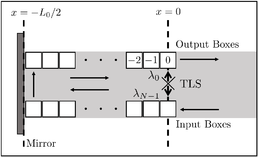
The two coupling functions for this system are
| (94) | ||||
where picks up the round trip phase of the photon in the interaction picture. Thus the coupling to the left is identical to the coupling without feedback, , and the coupling to the right is
| (95) | ||||
modified by the presence of the mirror.
Of course, does not occur for , so we reparamaterize and set the fictional box to be and box to be . Therefore, the interaction Hamiltonian for this scheme is
| (96) | ||||
where the directional subscript on has been dropped since there is only one set of boxes needed for this scheme.
IV.1.3 Scheme (iii): Two Waveguide-Coupled Two Level Systems Separated by a Time Delay
The third scheme of interest is two spatially separated TLSs in an open waveguide as depicted in Fig. 1(c). This system is commonly investigated under the assumption that the spatial separation is negligible to the dynamics of the system in order to recover Markovian dynamics (thus neglecting time retardation), and when the non-Markovian effects are included, it is commonly in the single excitation regime Sinha et al. 2020. We can relax this assumption with the SDW model and treat the non-Markovian effects from the separation of the TLSs with dynamics from up to four quanta in the entire system included (one in each TLS and two in the waveguide). The approach to modelling this system is similar to that of scheme (i), but now more than one box is needed to model the waveguide. Instead, boxes are introduced which span the distance between the two TLSs, shown schematically in Fig. 17.

There are now four coupling functions which must be converted into their respective spatial coupling functions. These coupling functions are presented in Eq. (28), and following a similar approach to the previous two sections, the interaction Hamiltonian in the SDW model is
| (97) | ||||
IV.2 Introducing Lindblad Output Channels
A central result of previous studies on coherent feedback systems is the ability to tune the phase of the returning feedback to enhance or suppress the output from the system. However, it is important to note that in physically realized systems, such as semiconductor quantum dots Gustin and Hughes 2018; Iles-Smith et al. 2017; Kuhlmann et al. 2013; Ramsay et al. 2010; Grange et al. 2017; Lodahl et al. 2015; Vagov et al. 2002; Förstner et al. 2003; Besombes et al. 2001; Türschmann et al. 2019, feedback systems are ultimately less effective when one accounts for dissipation processes such as off-chip decay from the TLS and pure dephasing. To include these processes in the SDW model, our algorithm is amended to include Lindblad quantum jump operators from conventional QT theory Dalibard et al. 1992; Tian and Carmichael 1992; Dum et al. 1992.
As an example, the previous schemes can be augmented by two quantum jump operators , representing off-chip decay from the TLS with rate , and , representing pure dephasing in the TLS with rate . It is important to note that the MPS approach neglects these terms and it is not clear how to include them in a numerically efficient way. In contrast, due to the already stochastic nature of the SDW model, including these output channels is quite natural and is one of the major advantages of exploiting QT theory to model waveguide QED.
In order to include these jumps, the algorithm’s first step must be modified by evolving each QT under a non-Hermitian effective Hamiltonian,
| (98) |
This evolution is further modified by stochastically introducing quantum jumps with a jump probability of
| (99) |
for the time step beginning at . If a jump is determined to occur, either or is chosen to be applied to the system according to their relative probabilities. Note, an alternative approach to include the above processes is to add further streams of little boxes, one stream for each additional decay or dephasing channel. However, we find our presented QT formalism to be more intuitive.
Since neither the evolution under or applying either quantum jump preserves the state norm, before moving on to the measurement of the final box in the second step of the algorithm, the state must be renormalized. Thus there must be two renormalizations during each step of the system evolution.
It is also important to note that, unlike in typical QT theory, if a quantum jump occurs, the waveguide Hamiltonian is still applied to the system, i.e., the boxes still shift. For a typical QT, if a jump occurs, the Hamiltonian is not applied to the system and instead the jump operator is applied. If this were to be followed for this model with feedback, then the feedback would return to the system at irregular times. Therefore, the waveguide Hamiltonian must be decoupled from the system and interaction Hamiltonians in order to maintain a consistent round trip time for the feedback.
IV.3 Implementation in Python
One of the major benefits of the SDW model is the ease of implementing the model in the users preferred coding language, especially if the user is familiar with QTs in general. Similar to our MPS implementation, our SDW implementation uses Python 3.7, which exploits its straightforward parallelization abilities and the sparse matrix capabilities of scipy.
To begin a simulation, the ket vector is initialized as an outer product of and , which is represented as a vector of length ; here the size of the QO system basis and the size of the waveguide basis. Note that is used in the factorial because the limit of photons in the waveguide encompasses both directions of field propagation in the loop (the is dropped for the feedback scheme since there is only one row of boxes). To give an example, for a typical simulation, we would choose 20 boxes () and allow for two photons in the loop () which gives a vector length of 422 for the single TLS with feedback and 3284 for two TLSs in an open waveguide. The evolution under is done similarly to our MPS implementation by utilizing the exponential function in scipy linalg, but we also convert it into a sparse matrix to save both memory and computation time since there are many levels of the ket vector which do not interact.
The simulation then runs by following the algorithm described in Sec. IV.1, implementing each time step (with Lindblad output channels included) until the desired end time is reached. First, there is a check for whether a quantum jump from the Lindblad output channels occurs, with probability ((99)). To do this check, a uniformly distributed random number, , is generated and compared against . If then a jump occurs, with the responsible jump operator chosen from their respective relative probabilities compared against a second uniformly distributed random number. Otherwise, if , then the system ket vector is evolved by direct multiplication of and then renormalized. Note that this step can be done with a smaller time step, , multiple times per large time step in order to resolve fast system Hamiltonian dynamics. Other methods of evolution can be used such as various Runge-Kutte approaches, however these require a larger number of calculations per time step and can slow down the numerics significantly for small gains in accuracy. Next, a direct measurement of the output boxes is taken to determine if a photon leaves the system from the waveguide. This is implemented similarly to the Lindblad jump operators with the probabilities now given by . Penultimately, the waveguide boxes are all shifted forward, and lastly, the ket vector is renormalized again.
The benefits of this implementation is that essentially each step of the code is obtained by simply writing down the explicit mathematical calculation that needs to be done without any outside functions. This makes the implementation quite easy and transparent for a simple system. The complexity arises as the system of interest becomes more intricate, for example through the inclusion of more Lindblad output channels or complex QO systems. Also, since the ket vector is known at each time step, any desired observables can be calculated either during or after the trajectory.
Of course, since each QT simulated is a single realization of the scheme of interest, in order to recover the ensemble average dynamics these trajectories must be averaged over a large number of realizations. Depending on the system dynamics or the desired precision of the observable, this can require anywhere from 500 to 10000 trajectories. Since each trajectory is inherently independent of the other trajectories, this implementation is a prime candidate for parallelization across multiple CPUs which we have done using the mpi4py package for Python. This can also make use of the multithreading on a single high-performance workstation or the many nodes of a computing cluster.
V Results
In this section, we present numerical results of the two methods discussed in detail above. For convenience, we will present the graphical results in normalized units, in terms of , defined from: , , and .
V.1 Single two level system in a waveguide with and without a time-delayed feedback: vacuum dynamics
We will first explore the case of a single TLS in a waveguide, with and without feedback, beginning with the simple spontaneous emission dynamics in vacuum.
As discussed earlier, since the SDW model computes stochastic dynamics, expectation values can be obtained from an average over a finite number of trajectories. To make this clear, at the few QT level, in Fig. 18, we show single trajectories calculated with this model for a TLS in an infinite waveguide and for a half open waveguide with a feedback delay (see sections II.1 and II.2), with and . We also compare these with the direct results given by the MPS, which shows a smooth decay in the case of no feedback, and population trapping for the case of feedback, which recovers previous vacuum results that have been reported elsewhere Kabuss et al. 2015; Carmele et al. 2013; Crowder et al. 2020. Since we only show a single QT (which is deliberate), the results obviously do not overlap, since when one quantum jump happens, the TLS population simply decays to the ground or becomes trapped. However, for a larger number of trajectories, we recover excellent agreement from both the MPS and SDW models as shown below.
Note that standard QTs for spontaneous emission begin as horizontal lines with no exponential decay. In the present case, the exponential behaviour occurs because there are 20 space bins interacting with the TLS before the interaction with the output bin begins; thus, the QTs are effectively conditioned on photon counts made downstream from the TLS.

In Fig. 20, we next study the same TLS decay for different feedback phases, yielding destructive interference with and constructive interference with , and show how the number of QT averages affects the results when comparing with the MPSs. We now see how the phase can completely change the trapping scenario causing a faster decay with feedback when . The MPS case is compared with 3 different cases for the SDW model, where 10, 100 and 2000 trajectories are considered. It can be seen that both methods agree extremely well in when , and we also show that both methods recover the simple analytical solution with no feedback, namely . Note that there are other non-Markovian systems that lead to TLS population trapping, such as fractional decay near the edge of a photonic bandgap John and Quang 1994; Nabiev et al. 1993, though in practise these would be very difficult to realize Kristensen et al. 2008, most notably due to structural disorder Hughes et al. 2005.
Now that we have verified that both approaches can yield the same predictions for the vacuum dynamics, it is also important to compare the computational efficiencies, as well as the ease of numerical implementation (which we have discussed earlier). For these vacuum examples of a single TLS in a waveguide, with and without feedback, the computational run times are compared in Tables 2 and 2. All the examples are run on the same computer workstation (125.6GB RAM, 3.70GHz, 16 cores).
| Model | Run Time (s) | |
|---|---|---|
| 10 | 0.25 | |
| SDW | 100 | 1.04 |
| 2000 | 14.22 | |
| MPS | 0.11 |
| Model | # of | Run Time (s) | |
|---|---|---|---|
| trajectories | |||
| 10 | 0.15 | 0.24 | |
| SDW | 100 | 0.69 | 1.76 |
| 2000 | 12.66 | 33.56 | |
| MPS | 1.18 | 1.30 | |
In the infinite waveguide case (Table 2), the MPS code is faster than any of the cases given with the SDW. Once the feedback is introduced into the MPS approach, as each time step involves more operations, the MPS code slows down. However, it is still comparable to around 100 trajectories.


While the MPS approach appears to be faster for the presented examples, they are clearly both efficient, and it is important to note that the computational implementation and intuitive understanding is much more complex. In addition, the SDW model can easily add in additional dissipation processes that are known to be important for connecting to real experiments, including off-chip photon decay and pure dephasing – the latter process is a well known feature with solid state quantum bits (quantum dots) Gustin and Hughes 2018; Iles-Smith et al. 2017; Kuhlmann et al. 2013; Ramsay et al. 2010; Grange et al. 2017; Lodahl et al. 2015; Vagov et al. 2002; Förstner et al. 2003; Besombes et al. 2001; Türschmann et al. 2019. As remarked earlier, implementing such processes with MPSs is not well developed and non trivial. To demonstrate the role of these processes, Fig. 20 shows the behavior of the decay of a TLS in a waveguide with a coherent feedback when these two effects are considered, separately. Indeed, in both cases, we see that these additional dissipation channels break the regime of perfect TLS population trapping, and it is essential to realize that these dephaning processes set a limit on how well one can exploit feedback in general. The run times increase around four times when these effects are added to the system, for the same parameters as the ones shown in Table 2 with ; this increase is more than reasonable given the complexity of the open system we are modelling, and the simulations are still efficient, even on a single computer.
It is also interesting to note that the role of and are qualitatively different in how they affect the trapping condition. This is because the process affects both the population decay and the coherence, while the pure dephasing does not directly reduce the population, but instead dephases the coherence that is necessary for population trapping. Thus the effect of off-chip decay is more problematic, though both processes lead to an overall decay of the trapped state.
V.2 Single two level system in a waveguide with and without a time-delayed feedback: nonlinear dynamics with a coherent pump field
Now that we have studied the vacuum decay dynamics of the TLS population, which can also easily be described with classical linear response theories Hughes 2007, the real power of our presented waveguide QED methods is in their ability to describe nonlinear effects beyond a single quantum, namely unique quantum nonlinear effects that have no classical counterpart. As an example, one can explicitly include one photon in the feedback loop, and the TLS or/and a side coupled cavity Crowder et al. 2020, which goes beyond the one quanta limit. Thus we next add a coherent pump field to the system Hamiltonian to access the quantum nonlinear regime.
Note, one of the main advantages of using MPSs is that there is no restriction on the number of photons considered in the waveguide (subject to computational restrictions inherent in the method), while in the SDW model we are restricted to one or two photons in the waveguide for this study; the extension to include three or more photons is possible, but the computational overhead may be considerable. However, it is very insightful to explicitly see the differences between between the 1 photon and 2 photon results, and often 2 photons plus the TLS excitations is enough for many few photon descriptions, even under extreme conditions (as we show below).
Figures 22 and 22 show coherent pump examples for the large drive strengths of and , respectively, which easily break a weak excitation approximation (when the TLS is basically in the classical harmonic oscillator regime). First, in Fig. 22, three different feedback lengths are considered for the same drive, yielding feedback times of . It can be seen that, as the feedback time increases, the results with 1 photon deviate from the MPS model and the 2 photon SDW results, and thus becomes incorrect. However, the 2 photon case seems to agree well with the MPS model, showing that this approximation is very accurate here. We also highlight that for longer feedback loops, the SDW model becomes slower, especially in the case of the SDW with two photons. Physically, as the length of the feedback loop increases, the probability of having two photons in the waveguide increases as well, making the approach in which two photons are considered more accurate. Table 3 gives a summary of computational run times for the two models.
In Fig. 22, it is important to note that the 1 photon limit case gives perfect population trapping Grimsmo 2015; Kabuss et al. 2015, while there is no perfect trapping in the 2 photons case and the MPS solution, and a decay can be seen. This is expected as it is practically impossible to phase match at two different frequencies, when quantum nonlinearies become important. This multi-photon influence on feedback-induced population trapping is consistent with the results from Grimsmo Grimsmo 2015 (whose results were limited to the early transient regime, showing only a few cycles). Note also, when running these codes for a non-trapping situation (e.g., with ), we found that the breakdown of the one photon case is still important (though suppressed), and the 2 photon case again agrees quantitatively well with the MPS result.
| Model | # Photons | Run Time (s) |
|---|---|---|
| SDW | 1 | 63.10 |
| 2 | 693.89 | |
| MPS | 43.43 |
In Fig. 22, we now apply an even larger pump field () on the same system. We see again, that even in the very strong field regime, the 2 photon SDW model is very accurate (agrees quantitatively well with the MPS results). However, we note the 2 photon SDW model needs more trajectories () to recover an accurate ensemble average, and a smaller time step in general, causing the SDW code to become somewhat slow and require more computational memory for accurate results; as an example, with a single multi-core workstation, in this case the run time for the SDW is 2406s (for a time step ) whereas the MPS code only takes 108s to run. Nevertheless, this is a very difficult nonlinear QO dynamic to model, and most other approaches to this problem would run into simulate computational problems or would not even be tractable (note we are also simulating for relatively long time scales with multiple oscillations). In addition, the longer feedback results are likely not as practical for applications, especially when one considers other realistic scattering processes (which are difficult for MPSs to handle).
V.3 Two coupled two level systems in a waveguide with a finite delay time between them
Next, we consider two TLSs in a waveguide (see Sec. II.3), with a finite separation between them. This example is a good test-best for beginning to exploit many-body interactions beyond the instantaneous coupling limit (an approximation that is frequently made when considering collective effects in the nonlinear regime). It is also a pedagogically important example, since it is known to produce sub-radiant and super-radiant Dicke states Dinc and Brańczyk 2019; Zhang and Mølmer 2019; Sinha et al. 2020, bound states in the regime of ultrastrong waveguide QED Román-Roche et al. 2020; Mukhopadhyay and Agarwal 2019, and cause complex waveguide-mediated phase coupling Cheng et al. 2017. For this system, we will again consider both vacuum dynamics and the case with strong optical pumping, as well as investigate the role of pure dephasing.


In Fig. 23, we first show results for the vacuum decay case, assuming the same decay rate for both TLSs (this is not a model restriction in either model). We start with the two TLSs in the excited state (Fig. 23(a)), and show how they decay equally, with a delay time of . Then, we consider a different initial condition where one TLS is in the ground state and the other one is in the excited state (Fig. 23(b)). It can be seen that both TLSs reach an equilibrium with a trapped TLS population, whose value decreases when the feedback time increases (cf. Figs. 23 (b) and (d)). Note the significant retardation oscillations that appear for the long delay time, initially causing a faster decay time. This shows that one can use the finite delay as a means to tune the emission dynamics of the distant TLS, similar to the effects of a distant mirror. Indeed, in the weak excitation regime, the other TLS acts a a resonant mirror (resonant scatterer), with a bandwidth that depends on the decay rate. Similar effects can be seen for TLSs embedded in cavities that are connected through a waveguide Yao and Hughes 2009a. All of these cases are calculated using MPSs and the SDW model, showing very good agreement for . Figure. 23(c) shows the impact of a pure dephasing rate in the TLSs for the same conditions as in (b). This is performed using the SDW code and shows how, in the same way as in the 1 TLS case, the population trapping (and entanglement) is destroyed in the long time limit when this effect is considered. The effect of adding an off-chip decay is very similar, so we do not bother showing it, and both effects cause a long time decay that depends on the additional decay rate. Further study in this coupling regime can be done, e.g., by changing the initial conditions and the phase between the TLSs, which would allow us to explore the impact on the known sub-radiant and super-radiant Dicke states Crowder 2020.
In this non-Markovian example, the decay rate of one TLS can exceed the one given by the Dicke superradiance due to field emitted from the other TLS (see also Figs. 23(d)). This can produce a constructive interference leading to a “super-superradiant” state. In Ref. Sinha et al. 2020 this is achieved in vacuum. We stress again that the dynamics in vacuum can easily be solved exactly as has been demonstrated in a number of works for coupling TLSs over macroscopic distances Yao and Hughes 2009a, where the retardation dynamics are exactly accounted and shown to play a qualitatively important role on two TLS coupling. While both our approaches here can also recover the super-superradiant state phenomena in vacuum, the real power of our QO waveguide approaches here is being apply to explore such regimes beyond the one quanta regime, and we will show examples of that below with CW pumping.
With regards to getting the same level of precision in both methods here, we can still use in the MPS approach, but we need to go to in the SDW model, thus increasing the run times. Run times are compared in Table 4, where the parallel version of the SDW code is considered (on a single computer). The long feedback case significantly slows down the SDW code, showing in this case the greatest difference between run times. However, the long feedback case is used more as an academic study, since the coherent interactions typically become less pronounced.
| Model | Run Time (s) | |
|---|---|---|
| SDW | 0.5 | 6.13 (, ) |
| MPS | 0.70 (, bond = 8) | |
| SDW | 2.5 | 381.63 (, ) |
| MPS | 4.37 (, bond = 8) |
We next consider two coupled TLS and a pumping field, with various results shown in Fig. 24. In Fig. 24(a), the case of a pump, , with a delay time, , is shown. This is calculated with both MPS and SDW codes. For the MPS, a bond dimension of 8 is required, taking 7.17s to run. For the SDW model, we need taking 189s in its parallelized version (all results for a single computer). It can be seen how the pump in one TLS affects the TLS population of the other one, exciting it with a coherent damped coupling and eventually reaching a steady state.
We now consider a stronger driven case in Fig. 24(b). It shows that, if the pump is too strong, an incoherent excitation of the second TLS appears, as the single TLS Rabi drive dominates the coherent oscillation of that population. It can be seen that the first TLS is apparently not affected by the second one, having a similar behaviour as in the case of having one driven TLS. The excitation of the second TLS is thus mainly through incoherent excitation.
After confirming the excellent agreement with both methods, we next consider a much longer delay time. In Fig. 24) (c), the population results with is shown. As we saw in the 1 TLS decay case, when the feedback increases substantially then the SDW code becomes much slower; also, here we have to consider the fact that there is also a significant pump field involved. For these reasons, this last example (c) is only run with the MPS approach. It is shown that for a longer feedback, the pumping scenario is similar to Fig. 24) (b), namely the response of the second TLS to continuous driving is through fluorescence from the first, eventually reaching the same steady state.
V.4 Entanglement entropy for two coupled two level systems in a waveguide: role of retardation
As a final application, we will study the entanglement between the 2 TLSs, for different delay times. The entanglement between the TLSs (joint system bin) and the waveguide can be measured through the entanglement entropy.
This is the Von Neumann entropy of the reduced density matrix Nielsen and Chuang 2009 (see also Eq (40)). The Von Neumann entropy for a state is,
| (100) |
which can be rewritten in terms of the Schmidt coefficients,
| (101) |
where indicates the position of the Schmidt coefficients in the diagonal matrix containing them.

Subsequently, the entanglement entropy between the TLSs bin and the waveguide can be written as follows Pichler and Zoller 2016,
| (102) |
where represents the reduced density matrix of the TLSs bin, and are the Schmidt coefficients corresponding to the TLSs. Depending on the dimensions of our TLS(s) bin there is a different maximum value of the entanglement entropy as it counts the number of entangled qubits between the parts of the system, being the maximum Nielsen and Chuang 2009 , where is the number of qubits. For example, in the case of 1 TLS, the maximum will be 1, and in the case of 2 TLS, the maximum will be 2.
Figure 25 shows the entanglement entropy between the TLSs bin and the waveguide for three different values of feedback (, and ), where it can be seen that the longer the feedback the lower the entanglement after reaching a steady state. For these examples, we use the MPS approach only, though clearly we would obtain the same result with the SDW approach.
VI Conclusions
We have presented two different models for solving quantum nonlinear light-matter in waveguide-QED systems, using MPSs and a SDW model. Both approaches are shown to efficiently describe the complicated non-Markovian cases of a time-delayed coherent feedback and two spatially separated TLSs. We applied these models to study three different topical systems in waveguide quantum circuits, including a TLS coupled to an infinite waveguide, a TLS coupled to a semi-infinite waveguide (with a time-delayed feedback), and two spatially separated TLS coupled to an infinite waveguide. Both methods include waveguide photons that are quantized at the system level and, importantly, can explore both linear and nonlinear quantum regimes. While the MPS approach is intrinsically non-Markovian, the SDW model solves Markovian equations of motion and exploits QT theory which also provides physical insight into the underlying stochastic dynamics Whalen et al. 2017.
After presenting the theory of MPSs and the SDW model, results were shown and compared directly for the three QED-waveguide systems of interest. Numerically, we find excellent agreement between both methods if the required number of waveguide photons is included in the SDW model, which works remarkably well with up to two photons in the loop, even under extreme pumping conditions. The SDW model also allows us to easily identify the differences between a one photon and a two photon approximation, yielding information about the role of two photon interference effects. For the case of one TLS and a time-delayed feedback, we have studied both the vacuum dynamics and nonlinear dynamics, verifying that the one-photon-in-the loop approximation breaks down in the presence of a strong pumping field. We also show how both methods can efficiently track the population trapped state, easily yielding coherent oscillations over a large number of periods. In addition, it was shown how two spatially-separated TLSs can be efficiently modelled with both approaches, showing again the vacuum dynamics and nonlinear quantum dynamics with a coherent pump field. We investigated the role of retardation, and briefly discussed how to quantify the entanglement entropy between the TLSs and the waveguide, with various delay times (spatial separations).
While we have shown that both approaches offer excellent complimentary information for modelling system-level waveguide QED, each has certain advantages and disadvantages for studying waveguide QED systems. The MPS model, although significantly more complicated to implement, offers faster run-time results in most of the cases studied in our paper, for the same level of precision. This becomes more noticeable when we increase the feedback length or/and if the system is driven by a very strong pump field. In these cases, the SDW model can run into computational memory problems; in contrast, in the MPS case, although the run times increase, there are no memory problems found for the examples presented. On the other hand, smaller delay times are more practical anyway. The SDW model also has some notable advantages over MPSs: (i) it can show results for different levels of approximation more clearly, such as results with one photon or two photons in the loop; (ii) it is far easier to implement computationally, is perfectly parallelizable, and uses well known techniques in quantum optics, such as QT theory; (iii) the equations are actually all Markovian, even though retardation effects are fully accounted for; (iv) the ease of adding in other dissipation channels such as off-chip decay and pure dephasing is fairly straightforward. In this latter case, we demonstrated the importance of these effects as an important limit to creating population trapped states and entangled qubits. For connecting to real experiments, such as with semiconductor quantum dots, including such processes is critical.
Overall, our paper shows how one can implement both these two different methods to accurately model complicated waveguide QED systems, which can work together as powerful and complementary models in quantum optics. Indeed, as we have demonstrated, these methods can be used to improve our understanding and exploitation of complex non-Markovian feedback systems. Both the SDW model and the MPS model can also support the addition of more complicated circuits, including two TLSs with a mirror-based coherent feedback, pulsed excitation, and input-output theory with input photon states. Although we find that the approximation to two photons is highly accurate for the results presented in this paper, the presence of more photons can become important in other cases, giving the opportunity to describe more complex systems in future work, e.g. three quantum emitters (TLSs) in a waveguide Carmele et al. 2020 (where the side atoms can behave like mirrors in cavity QED Mirhosseini et al. 2019), a higher number of qubits Albrecht et al. 2019; Finsterhölzl et al. 2020, and 1D atomic arrays Masson and Asenjo-Garcia 2019; Wang et al. 2020.
Acknowledgements.
This work was funded by the Natural Sciences and Engineering Research Council of Canada, the Canadian Foundation for Innovation and Queen’s University, Canada. Howard Carmichael acknowledges the support of the New Zealand Tertiary Education Committee through the Dodd-Walls Centre for Photonic and Quantum Technologies. We thank Nir Rotenberg for useful comments.References
- Hughes (2004) S. Hughes, Enhanced single-photon emission from quantum dots in photonic crystal waveguides and nanocavities, Optics Letters 29, 2659 (2004).
- Shen and Fan (2007a) J.-T. Shen and S. Fan, Strongly correlated multiparticle transport in one dimension through a quantum impurity, Phys. Rev. A 76, 062709 (2007a).
- Shen and Fan (2007b) J.-T. Shen and S. Fan, Strongly correlated two-photon transport in a one-dimensional waveguide coupled to a two-level system, Phys. Rev. Lett. 98, 153003 (2007b).
- Zheng et al. (2010) H. Zheng, D. J. Gauthier, and H. U. Baranger, Waveguide QED: Many-body bound-state effects in coherent and fock-state scattering from a two-level system, Phys. Rev. A 82, 063816 (2010).
- Witthaut and Sørensen (2010) D. Witthaut and A. S. Sørensen, Photon scattering by a three-level emitter in a one-dimensional waveguide, New Journal of Physics 12, 043052 (2010).
- Longo et al. (2011) P. Longo, P. Schmitteckert, and K. Busch, Few-photon transport in low-dimensional systems, Phys. Rev. A 83, 063828 (2011).
- Roy (2011) D. Roy, Two-photon scattering by a driven three-level emitter in a one-dimensional waveguide and electromagnetically induced transparency, Phys. Rev. Lett. 106, 053601 (2011).
- Sanchez-Burillo et al. (2014) E. Sanchez-Burillo, D. Zueco, J. J. Garcia-Ripoll, and L. Martin-Moreno, Scattering in the ultrastrong regime: Nonlinear optics with one photon, Phys. Rev. Lett. 113, 263604 (2014).
- Calajó et al. (2016) G. Calajó, F. Ciccarello, D. Chang, and P. Rabl, Atom-field dressed states in slow-light waveguide qed, Phys. Rev. A 93, 033833 (2016).
- Pichler and Zoller (2016) H. Pichler and P. Zoller, Photonic circuits with time delays and quantum feedback, Phys. Rev. Lett. 116, 093601 (2016).
- Manga Rao and Hughes (2007) V. S. C. Manga Rao and S. Hughes, Single quantum-dot purcell factor and factor in a photonic crystal waveguide, Phys. Rev. B 75, 205437 (2007).
- Lund-Hansen et al. (2008) T. Lund-Hansen, S. Stobbe, B. Julsgaard, H. Thyrrestrup, T. Sünner, M. Kamp, A. Forchel, and P. Lodahl, Experimental realization of highly efficient broadband coupling of single quantum dots to a photonic crystal waveguide, Phys. Rev. Lett. 101, 113903 (2008).
- Laucht et al. (2012) A. Laucht, S. Pütz, T. Günthner, N. Hauke, R. Saive, S. Frédérick, M. Bichler, M.-C. Amann, A. W. Holleitner, M. Kaniber, and J. J. Finley, A waveguide-coupled on-chip single-photon source, Phys. Rev. X 2, 011014 (2012).
- Gardiner and Zoller (2010) C. W. Gardiner and P. Zoller, Quantum noise: a handbook of Markovian and non-Markovian quantum stochastic methods with applications to quantum optics (Springer, Berlin, 2010).
- Droenner et al. (2019) L. Droenner, N. L. Naumann, E. Schöll, A. Knorr, and A. Carmele, Quantum Pyragas control: Selective control of individual photon probabilities, Physical Review A 99, 023840 (2019).
- Crowder et al. (2020) G. Crowder, H. Carmichael, and S. Hughes, Quantum trajectory theory of few-photon cavity-QED systems with a time-delayed coherent feedback, Physical Review A 101, 023807 (2020).
- Dorner and Zoller (2002) U. Dorner and P. Zoller, Laser-driven atoms in half-cavities, Physical Review A 66, 023816 (2002).
- Tufarelli et al. (2013) T. Tufarelli, F. Ciccarello, and M. S. Kim, Dynamics of spontaneous emission in a single-end photonic waveguide, Physical Review A 87, 013820 (2013).
- Carmele et al. (2013) A. Carmele, J. Kabuss, F. Schulze, S. Reitzenstein, and A. Knorr, Single photon delayed feedback: A way to stabilize intrinsic quantum cavity electrodynamics, Phys. Rev. Lett. 110, 013601 (2013).
- Német et al. (2019) N. Német, A. Carmele, S. Parkins, and A. Knorr, Comparison between continuous- and discrete-mode coherent feedback for the Jaynes-Cummings model, Physical Review A 100, 023805 (2019).
- Grimsmo (2015) A. L. Grimsmo, Time-delayed quantum feedback control, Phys. Rev. Lett. 115, 060402 (2015).
- Whalen et al. (2017) S. J. Whalen, A. L. Grimsmo, and H. J. Carmichael, Open quantum systems with delayed coherent feedback, Quantum Science and Technology 2, 044008 (2017).
- Chalabi and Waks (2018) H. Chalabi and E. Waks, Interaction of photons with a coupled atom-cavity system through a bidirectional time-delayed feedback, Phys. Rev. A 98, 063832 (2018).
- Kubanek et al. (2009) A. Kubanek, M. Koch, C. Sames, A. Ourjoumtsev, P. W. H. Pinkse, K. Murr, and G. Rempe, Photon-by-photon feedback control of a single-atom trajectory, Nature 462, 898 (2009).
- Gillett et al. (2010) G. G. Gillett, R. B. Dalton, B. P. Lanyon, M. P. Almeida, M. Barbieri, G. J. Pryde, J. L. O’Brien, K. J. Resch, S. D. Bartlett, and A. G. White, Experimental feedback control of quantum systems using weak measurements, Phys. Rev. Lett. 104, 080503 (2010).
- Brandes (2010) T. Brandes, Feedback control of quantum transport, Phys. Rev. Lett. 105, 060602 (2010).
- Balouchi and Jacobs (2017) A. Balouchi and K. Jacobs, Coherent versus measurement-based feedback for controlling a single qubit, Quantum Science and Technology 2, 025001 (2017).
- Calajó et al. (2019) G. Calajó, Y.-L. L. Fang, H. U. Baranger, and F. Ciccarello, Exciting a Bound State in the Continuum through Multiphoton Scattering Plus Delayed Quantum Feedback, Physical Review Letters 122, 073601 (2019).
- Yao and Hughes (2009a) P. Yao and S. Hughes, Macroscopic entanglement and violation of bell’s inequalities between two spatially separated quantum dots in a planar photonic crystal system, Optics Express 17, 11505 (2009a).
- Hein et al. (2016) S. M. Hein, A. Carmele, and A. Knorr, Creation and control of entanglement by time-delayed quantum-coherent feedback, in Physics and Simulation of Optoelectronic Devices XXIV, edited by B. Witzigmann, M. Osiński, and Y. Arakawa (SPIE, 2016).
- Buckley et al. (2012) S. Buckley, K. Rivoire, and J. Vučković, Engineered quantum dot single-photon sources, Reports on Progress in Physics 75, 126503 (2012).
- Matthiesen et al. (2012) C. Matthiesen, A. N. Vamivakas, and M. Atatüre, Subnatural linewidth single photons from a quantum dot, Phys. Rev. Lett. 108, 093602 (2012).
- Heinze et al. (2015) D. Heinze, D. Breddermann, A. Zrenner, and S. Schumacher, A quantum dot single-photon source with on-the-fly all-optical polarization control and timed emission, Nature Communications 6 (2015).
- Türschmann et al. (2019) P. Türschmann, H. L. Jeannic, S. F. Simonsen, H. R. Haakh, S. Götzinger, V. Sandoghdar, P. Lodahl, and N. Rotenberg, Coherent nonlinear optics of quantum emitters in nanophotonic waveguides, Nanophotonics 8, 1641 (2019).
- Gu et al. (2017) X. Gu, A. F. Kockum, A. Miranowicz, Y. xi Liu, and F. Nori, Microwave photonics with superconducting quantum circuits, Physics Reports 718-719, 1 (2017).
- Kockum et al. (2018) A. F. Kockum, G. Johansson, and F. Nori, Decoherence-free interaction between giant atoms in waveguide quantum electrodynamics, Phys. Rev. Lett. 120, 140404 (2018).
- Kannan et al. (2020) B. Kannan, M. J. Ruckriegel, D. L. Campbell, A. F. Kockum, J. Braumüller, D. K. Kim, M. Kjaergaard, P. Krantz, A. Melville, B. M. Niedzielski, A. Vepsäläinen, R. Winik, J. L. Yoder, F. Nori, T. P. Orlando, S. Gustavsson, and W. D. Oliver, Waveguide quantum electrodynamics with superconducting artificial giant atoms, Nature 583, 775 (2020).
- Yang et al. (2018) C. Yang, F. C. Binder, V. Narasimhachar, and M. Gu, Matrix product states for quantum stochastic modeling, Physical Review Letters 121, 260602 (2018).
- Vanderstraeten (2017) L. Vanderstraeten, Tensor Network States and Effective Particles for Low Dimensional Quantum Spin Systems (Springer, Cham, 2017).
- Naumann et al. (2017) N. L. Naumann, S. M. Hein, M. Kraft, A. Knorr, and A. Carmele, Feedback control of photon statistics, in Physics and Simulation of Optoelectronic Devices XXV, Vol. 10098 (International Society for Optics and Photonics, 2017) p. 100980N.
- Ciccarello (2017) F. Ciccarello, Collision models in quantum optics, QMTR 4, 53 (2017).
- Whalen (2019) S. J. Whalen, Collision model for non-markovian quantum trajectories, Phys. Rev. A 100, 052113 (2019).
- Crowder (2020) G. Crowder, Quantum Trajectory Theory of Open Cavity-QED Systems with a Time Delayed Coherent Optical Feedback, Master’s thesis, Queen’s University at Kingston (2020).
- Cilluffo et al. (2020) D. Cilluffo, A. Carollo, S. Lorenzo, J. A. Gross, G. M. Palma, and F. Ciccarello, Collisional picture of quantum optics with giant emitters, arXiv:2006.08631 [quant-ph] (2020).
- Orús (2014) R. Orús, A practical introduction to tensor networks: Matrix product states and projected entangled pair states, Annals of Physics 349, 117 (2014).
- Droenner (2019) L. J. Droenner, Out-of-equilibrium dynamics of open quantum many-body systems, Doctoral thesis, Technischen Universität Berlin (2019).
- Eduardo (2017) S. B. Eduardo, One-dimensional few-photon scattering (Prensas de la Universidad de Zaragoza, Zaragoza, 2017).
- Brun (2002) T. A. Brun, A simple model of quantum trajectories, American Journal of Physics 70, 719 (2002).
- Kretschmer et al. (2016) S. Kretschmer, K. Luoma, and W. T. Strunz, Collision model for non-Markovian quantum dynamics, Physical Review A 94, 012106 (2016).
- Gustin and Hughes (2018) C. Gustin and S. Hughes, Pulsed excitation dynamics in quantum-dot–cavity systems: Limits to optimizing the fidelity of on-demand single-photon sources, Phys. Rev. B 98, 045309 (2018).
- Iles-Smith et al. (2017) J. Iles-Smith, D. P. S. McCutcheon, A. Nazir, and J. Mørk, Phonon scattering inhibits simultaneous near-unity efficiency and indistinguishability in semiconductor single-photon sources, Nature Photonics 11, 521 (2017).
- Kuhlmann et al. (2013) A. V. Kuhlmann, J. Houel, A. Ludwig, L. Greuter, D. Reuter, A. D. Wieck, M. Poggio, and R. J. Warburton, Charge noise and spin noise in a semiconductor quantum device, Nature Physics 9, 570 (2013).
- Ramsay et al. (2010) A. J. Ramsay, A. V. Gopal, E. M. Gauger, A. Nazir, B. W. Lovett, A. M. Fox, and M. S. Skolnick, Damping of exciton rabi rotations by acoustic phonons in optically excited quantum dots, Phys. Rev. Lett. 104, 017402 (2010).
- Grange et al. (2017) T. Grange, N. Somaschi, C. Antón, L. De Santis, G. Coppola, V. Giesz, A. Lemaître, I. Sagnes, A. Auffèves, and P. Senellart, Reducing phonon-induced decoherence in solid-state single-photon sources with cavity quantum electrodynamics, Phys. Rev. Lett. 118, 253602 (2017).
- Lodahl et al. (2015) P. Lodahl, S. Mahmoodian, and S. Stobbe, Interfacing single photons and single quantum dots with photonic nanostructures, Rev. Mod. Phys. 87, 347 (2015).
- Vagov et al. (2002) A. Vagov, V. M. Axt, and T. Kuhn, Electron-phonon dynamics in optically excited quantum dots: Exact solution for multiple ultrashort laser pulses, Phys. Rev. B 66, 165312 (2002).
- Förstner et al. (2003) J. Förstner, C. Weber, J. Danckwerts, and A. Knorr, Phonon-assisted damping of rabi oscillations in semiconductor quantum dots, Phys. Rev. Lett. 91, 127401 (2003).
- Besombes et al. (2001) L. Besombes, K. Kheng, L. Marsal, and H. Mariette, Acoustic phonon broadening mechanism in single quantum dot emission, Phys. Rev. B 63, 155307 (2001).
- le Feber et al. (2015) B. le Feber, N. Rotenberg, and L. Kuipers, Nanophotonic control of circular dipole emission, Nature Communications 6, 10.1038/ncomms7695 (2015).
- Young et al. (2015) A. B. Young, A. C. T. Thijssen, D. M. Beggs, P. Androvitsaneas, L. Kuipers, J. G. Rarity, S. Hughes, and R. Oulton, Polarization engineering in photonic crystal waveguides for spin-photon entanglers, Phys. Rev. Lett. 115, 153901 (2015).
- Söllner et al. (2015) I. Söllner, S. Mahmoodian, S. L. Hansen, L. Midolo, A. Javadi, G. Kiršanskė, T. Pregnolato, H. El-Ella, E. H. Lee, J. D. Song, S. Stobbe, and P. Lodahl, Deterministic photon–emitter coupling in chiral photonic circuits, Nature Nanotechnology 10, 775 (2015).
- Barik et al. (2018) S. Barik, A. Karasahin, C. Flower, T. Cai, H. Miyake, W. DeGottardi, M. Hafezi, and E. Waks, A topological quantum optics interface, Science 359, 666 (2018).
- Lodahl et al. (2017) P. Lodahl, S. Mahmoodian, S. Stobbe, A. Rauschenbeutel, P. Schneeweiss, J. Volz, H. Pichler, and P. Zoller, Chiral quantum optics, Nature 541, 473 (2017).
- Bliokh and Nori (2012) K. Y. Bliokh and F. Nori, Transverse spin of a surface polariton, Phys. Rev. A 85, 061801 (2012).
- Coles et al. (2016) R. J. Coles, D. M. Price, J. E. Dixon, B. Royall, E. Clarke, P. Kok, M. S. Skolnick, A. M. Fox, and M. N. Makhonin, Chirality of nanophotonic waveguide with embedded quantum emitter for unidirectional spin transfer, Nature Communications 7, 10.1038/ncomms11183 (2016).
- Martin-Cano et al. (2019) D. Martin-Cano, H. R. Haakh, and N. Rotenberg, Chiral emission into nanophotonic resonators, ACS Photonics 6, 961 (2019).
- Orazbayev et al. (2018) B. Orazbayev, N. Kaina, and R. Fleury, Chiral waveguides for robust waveguiding at the deep subwavelength scale, Phys. Rev. Applied 10, 054069 (2018).
- Petersen et al. (2014) J. Petersen, J. Volz, and A. Rauschenbeutel, Chiral nanophotonic waveguide interface based on spin-orbit interaction of light, Science 346, 67 (2014).
- Yao and Hughes (2009b) P. Yao and S. Hughes, Controlled cavity qed and single-photon emission using a photonic-crystal waveguide cavity system, Phys. Rev. B 80, 165128 (2009b).
- Pichler et al. (2017) H. Pichler, S. Choi, P. Zoller, and M. D. Lukin, Universal photonic quantum computation via time-delayed feedback, PNAS 114, 11362 (2017).
- McCulloch (2007) I. P. McCulloch, From density-matrix renormalization group to matrix product states, Journal of Statistical Mechanics 2007 (10), P10014.
- Woolfe (2015) K. Woolfe, Matrix product operator simulations of quantum algorithms, Ph.D. thesis, University of Melbourne (2015).
- Schollwöck (2011) U. Schollwöck, The density-matrix renormalization group in the age of matrix product states, Annals of Physics 326, 96 (2011).
- Iblisdir et al. (2007) S. Iblisdir, R. Orús, and J. I. Latorre, Matrix product states algorithms and continuous systems, Physical Review B 75, 104305 (2007).
- Pavarini et al. (2013) E. Pavarini, E. Koch, and U. Schollwöck, Emergent phenomena in correlated matter: lecture notes of the Autumn School Correlated Electrons 2013 at Forschungszentrum Jülich, 23 – 27 September 2013, edited by Institute for Advanced Simulation, Schriften des Forschungszentrums Jülich Reihe Modeling and Simulation No. 3 (Forschungszentrum Jülich, Jülich, 2013).
- Vanderstraeten et al. (2019) L. Vanderstraeten, J. Haegeman, and F. Verstraete, Tangent-space methods for uniform matrix product states, SciPost Physics Lecture Notes , 7 (2019).
- Hubig et al. (2017) C. Hubig, I. P. McCulloch, and U. Schollwöck, Generic construction of efficient matrix product operators, Phys. Rev. B 95, 035129 (2017).
- Subaşı et al. (2019) Y. Subaşı, L. Cincio, and P. J. Coles, Entanglement spectroscopy with a depth-two quantum circuit, Journal of Physics A 52, 044001 (2019).
- Nielsen et al. (2003) M. A. Nielsen, C. M. Dawson, J. L. Dodd, A. Gilchrist, D. Mortimer, T. J. Osborne, M. J. Bremner, A. W. Harrow, and A. Hines, Quantum dynamics as a physical resource, Physical Review A 67, 052301 (2003).
- Band and Avishai (2013) Y. B. Band and Y. Avishai, Quantum mechanics with applications to nanotechnology and information science, 1st ed. (Academic Press, Amsterdam ; New York, 2013).
- Sánchez-Burillo et al. (2015) E. Sánchez-Burillo, J. García-Ripoll, L. Martín-Moreno, and D. Zueco, Nonlinear quantum optics in the (ultra)strong light–matter coupling, Faraday Discussions 178, 335 (2015).
- Xu and Fan (2018) S. Xu and S. Fan, Generate tensor network state by sequential single-photon scattering in waveguide QED systems, APL Photonics 3, 116102 (2018).
- Pfeifer et al. (2015) R. N. C. Pfeifer, G. Evenbly, S. Singh, and G. Vidal, NCON: A tensor network contractor for MATLAB, arXiv:1402.0939 (2015).
- Dalibard et al. (1992) J. Dalibard, Y. Castin, and K. Mølmer, Wave-function approach to dissipative processes in quantum optics, Phys. Rev. Lett. 68, 580 (1992).
- Tian and Carmichael (1992) L. Tian and H. J. Carmichael, Quantum trajectory simulations of two-state behavior in an optical cavity containing one atom, Phys. Rev. A 46, R6801 (1992).
- Dum et al. (1992) R. Dum, P. Zoller, and H. Ritsch, Monte carlo simulation of the atomic master equation for spontaneous emission, Phys. Rev. A 45, 4879 (1992).
- Sinha et al. (2020) K. Sinha, P. Meystre, E. A. Goldschmidt, F. K. Fatemi, S. L. Rolston, and P. Solano, Non-markovian collective emission from macroscopically separated emitters, Phys. Rev. Lett. 124, 043603 (2020).
- Kabuss et al. (2015) J. Kabuss, D. O. Krimer, S. Rotter, K. Stannigel, A. Knorr, and A. Carmele, Analytical study of quantum-feedback-enhanced rabi oscillations, Phys. Rev. A 92, 053801 (2015).
- John and Quang (1994) S. John and T. Quang, Spontaneous emission near the edge of a photonic band gap, Phys. Rev. A 50, 1764 (1994).
- Nabiev et al. (1993) R. F. Nabiev, P. Yeh, and J. J. Sanchez-Mondragon, Dynamics of the spontaneous emission of an atom into the photon-density-of-states gap: Solvable quantum-electrodynamical model, Phys. Rev. A 47, 3380 (1993).
- Kristensen et al. (2008) P. Kristensen, A. F. Koenderink, P. Lodahl, B. Tromborg, and J. Mørk, Fractional decay of quantum dots in real photonic crystals, Optics Letters 33, 1557 (2008).
- Hughes et al. (2005) S. Hughes, L. Ramunno, J. F. Young, and J. E. Sipe, Extrinsic optical scattering loss in photonic crystal waveguides: Role of fabrication disorder and photon group velocity, Phys. Rev. Lett. 94, 033903 (2005).
- Hughes (2007) S. Hughes, Coupled-cavity qed using planar photonic crystals, Phys. Rev. Lett. 98, 083603 (2007).
- Dinc and Brańczyk (2019) F. Dinc and A. M. Brańczyk, Non-markovian super-superradiance in a linear chain of up to 100 qubits, Phys. Rev. Research 1, 032042 (2019).
- Zhang and Mølmer (2019) Y.-X. Zhang and K. Mølmer, Theory of subradiant states of a one-dimensional two-level atom chain, Physical Review Letters 122, 203605 (2019).
- Román-Roche et al. (2020) J. Román-Roche, E. Sánchez-Burillo, and D. Zueco, Bound states in ultrastrong waveguide QED, Phys. Rev. A 102, 023702 (2020).
- Mukhopadhyay and Agarwal (2019) D. Mukhopadhyay and G. S. Agarwal, Multiple fano interferences due to waveguide-mediated phase coupling between atoms, Phys. Rev. A 100, 013812 (2019).
- Cheng et al. (2017) M.-T. Cheng, J. Xu, and G. S. Agarwal, Waveguide transport mediated by strong coupling with atoms, Physical Review A 95, 053807 (2017).
- Nielsen and Chuang (2009) M. A. Nielsen and I. L. Chuang, Quantum Computation and Quantum Information (Cambridge University Press, 2009).
- Carmele et al. (2020) A. Carmele, N. Nemet, V. Canela, and S. Parkins, Pronounced non-markovian features in multiply excited, multiple emitter waveguide qed: Retardation induced anomalous population trapping, Phys. Rev. Research 2, 013238 (2020).
- Mirhosseini et al. (2019) M. Mirhosseini, E. Kim, X. Zhang, A. Sipahigil, P. B. Dieterle, A. J. Keller, A. Asenjo-Garcia, D. E. Chang, and O. Painter, Cavity quantum electrodynamics with atom-like mirrors, Nature 569, 692 (2019).
- Albrecht et al. (2019) A. Albrecht, L. Henriet, A. Asenjo-Garcia, P. B. Dieterle, O. Painter, and D. E. Chang, Subradiant states of quantum bits coupled to a one-dimensional waveguide, New Journal of Physics 21, 025003 (2019).
- Finsterhölzl et al. (2020) R. Finsterhölzl, M. Katzer, A. Knorr, and A. Carmele, Using matrix-product states for open quantum many-body systems: Efficient algorithms for markovian and non-markovian time-evolution, Entropy 22, 984 (2020).
- Masson and Asenjo-Garcia (2019) S. J. Masson and A. Asenjo-Garcia, Atomic-waveguide quantum electrodynamics (2019), arXiv:1912.06234 .
- Wang et al. (2020) Z. Wang, T. Jaako, P. Kirton, and P. Rabl, Supercorrelated radiance in nonlinear photonic waveguides, Phys. Rev. Lett. 124, 213601 (2020).