跳到论文正文
W Papers独立论文阅读器 arXiv:2011.11800 论文正文 计算阅读时间 · 0%
引用这篇论文根据当前论文元数据生成,正式投稿前建议核对。


License: CC BY 4.0
arXiv:2011.11800v2 [math.FA] 12 Dec 2022

On Hastings’ approach to Lin’s Theorem for Almost Commuting Matrices

David Herrera Note: Rutgers University. dh708@math.rutgers.edu
August 11, 2026
Abstract

Lin’s theorem states that for all ϵ>0\epsilon>0, there is a δ>0\delta>0 such that for all n≥1n\geq 1 if self-adjoint contractions A,B∈Mn​(ℂ)A,B\in M_{n}(\mathbb{C}) satisfy ‖[A,B]‖<δ\|[A,B]\|<\delta then there are self-adjoint contractions A′,B′∈Mn​(ℂ)A^{\prime},B^{\prime}\in M_{n}(\mathbb{C}) with [A′,B′]=0[A^{\prime},B^{\prime}]=0 and ‖A−A′‖,‖B−B′‖<ϵ\|A-A^{\prime}\|,\|B-B^{\prime}\|<\epsilon. We present fully explained and corrected details of the approach in [29], which was the first version of Lin’s theorem to provide asymptotic estimates.

We also apply this method to the case where BB is a normal matrix with spectrum lying in some nice 1-dimensional subset of ℂ\mathbb{C}.

1 Introduction

The following is known as Lin’s theorem

Theorem 1.1.

If A,B∈Mn​(ℂ)A,B\in M_{n}(\mathbb{C}) are self-adjoint contractions with

‖[A,B]‖<δ,\|[A,B]\|<\delta,

then there are commuting self-adjoint A′,B′∈Mn​(ℂ)A^{\prime},B^{\prime}\in M_{n}(\mathbb{C}) such that

‖A−A′‖,‖B−B′‖<ϵ⁡(δ),\|A-A^{\prime}\|,\|B-B^{\prime}\|<\epsilon(\delta),

where limδ→0+ϵ⁡(δ)=0\lim_{\delta\to 0^{+}}\epsilon(\delta)=0.

It is important to note that ϵ⁡(δ)\epsilon(\delta) does not depend on nn. We will discuss results that depend on nn later. We formulated Lin’s theorem similar to [31], [34]. One can also express this result in terms of δ\delta depending on ϵ\epsilon as in the abstract.

If ‖[A,B]‖\|[A,B]\| is small, we refer to AA and BB as “almost commuting” and if there are nearby commuting matrices (with whatever specified properties), we refer to AA and BB as “nearly commuting”. In these terms, Lin’s theorem says that almost commuting Hermitian matrices (with bounded norm) are near Hermitian commuting matrices. Lin’s theorem can also be formulated in terms of almost normal matrices being nearly normal, where a matrix NN is almost normal if its self-commutator [N∗,N][N^{\ast},N] has small norm and NN is nearly normal if there is a normal matrix nearby NN.

Lin’s theorem is the positive answer to a question (for the operator norm) stated by Rosenthal in [44] in11 1 The dates stated in this paper use published dates and received dates when possible. 1969 and in 1976 was listed as one of various unsolved problems by Halmos in [27]. By the time that Lin’s proof appeared, there were various results that fell short of Lin’s theorem in important ways. Positive results were obtained when ϵ\epsilon is allowed to depend on nn and negative results were obtained when we are considering general self-adjoint operators acting on an infinite dimensional Hilbert space: [37] in 1969 (with the Euclidean norm) and [4] in 1974 (with the operator norm, with proof attributed to Halmos) presented a result with dimensional dependence of δ\delta. Also, [4] presented related results that fail in infinite dimensions and [6] in 1980 presented an example of an obstruction related to the Fredholm index in the infinite dimensional analogue to Lin’s theorem. In 1979, Pearcy and Shields in [41] gave the dimensional dependence of ϵ=((n−1)​δ/2)1/2\epsilon=((n-1)\delta/2)^{1/2}, but only used that one of the operators is assumed to be self-adjoint. The dependence of ϵ\epsilon on δ\delta has the optimal exponent for Lin’s theorem.

Davidson in [14] in 1985 provided an example of normal matrices (gotten by an approximation result of Berg in [7]) and a Hermitian matrices that almost commute but are not nearby commuting normal and Hermitian matrices using a spectral projection argument and a property of the shift on ℂn\mathbb{C}^{n}. This shows that the Pearcy and Shields result cannot be improved to remove its dimensional dependence, as we will discuss later. See Section 16 for more about generalizations.

In 1990, Szarek in [47] proved that Lin’s theorem holds for ϵ=c​(n1/2​δ)2/13\epsilon=c(n^{1/2}\delta)^{2/13}, where cc is some constant. Szarek states that the exponent of ϵ\epsilon can be reduced by using a more complicated argument but the aim was to use the approach discussed in [14] and the assumption that both operators are Hermitian to obtain stronger dimensional dependence than the counter-examples seen thus far had exhibited and hence “the situation in the Hermitian setting is completely different”.

In 1997, Lin in [35] provided a proof of Lin’s Theorem and in 1996 Friis and Rørdam in [23] published a simplified version of Lin’s result (referencing [35] which was to appear in Operator Algebras and Their Applications).

Up until this point, the proof of Lin’s theorem was abstract and neither gave the asymptotic dependence of ϵ\epsilon solely on δ\delta nor gave a way of constructing these matrices. In 2008, [28] by Hastings presented an approach whose starting point is similar to one of [14]’s reformulations of Lin’s theorem. [28] claimed to provide a constructive method of finding the nearby commuting matrices and also presenting an asymptotic dependence of ϵ\epsilon on δ\delta. The methods in [28] for a diagonal and tridiagonal pair of Hermitian matrices (which was already implicitly solved without the ideal exponent in [47]) held. However, the arguments for the general case were amended to try to resolve errors and consequently the main result changed. Namely, the most recent version of this paper, being [29] pre-published on arxiv.org in 2010, states similar statements for asymptotic dependence of ϵ\epsilon on δ\delta but not that the result is constructive and the dependence only holds for δ\delta small enough (but neither how small nor any constant in the dependence of ϵ\epsilon on δ\delta is given).

In 2015, Kachkovskiy and Safarov in [34] proved a result that not only gives the optimal homogeneous dependence of ϵ\epsilon on δ\delta of ϵ=C​o​n​s​t.δ1/2\epsilon=Const.\delta^{1/2} and simultaneously addresses the infinite dimensional situation where the index obstruction of Berg and Olsen applies. The proof also appears to be essentially constructive if the nearby commuting matrices sought for belong to the von Neumann algebra generated by the two almost commuting matrices.

A list of applications of almost/nearly commuting matrices can be found in the introduction of [36]. The first example given there is related to a paper of von Neumann concerning macroscopic observables. Although at least three almost commuting Hermitian matrices are not necessarily nearly commuting, Ogata in [39] showed that a special case of this related to von Neumann’s example is true.

There have also been many “spin-offs” of this problem, involving different norms, algebraic objects that are not operators on a Hilbert space, and for bounded operators on an infinite dimensional Hilbert space. Notable mentions are that Lin’s theorem holds for the normalized Schatten-pp norms ([45]) and that Lin’s theorem for the normalized Hilbert-Schmidt norm holds for multiple Hermitian matrices ([24]).

Given that this problem has effectively been solved in the general case, one might wonder why would one explore Hastings’ earlier approach that does not provide the optimal exponent and does not provide a constructive proof unless relying on [34] as a black-box. One reason is that it demonstrates how to obtain an asymptotic estimate from even the version of Lin’s theorem stated without any explicit estimate provided. That is, some of the arguments in Hastings’ approach are interesting in and of themselves.

A main reason that the author still finds Hastings’ approach interesting is that the unlike the approach of [34], Hastings’ approach involves following one of Davidson’s reformulations of Lin’s theorem in terms of constructing a certain almost invariant subspace of a block tridiagonal matrix. Szarek seems to be the first to effectively use this reformulation and Hastings provided a nice proof of this lemma in the case of tridiagonal matrices in [29]. Although Lin’s theorem has been proved with the optimal asymptotic exponent, it is still an open problem whether the exponent in this reformulation of Lin’s theorem can be improved. See Remark 6.5 below. So, we still have an interesting matrix theory question to explore.

Also, even in the case that one uses [34]’s result, the structure gotten by Davidson’s reformulation of Lin’s theorem is nice enough that one might find reason to make a compromise and apply [34]’s result to Davidson’s reformulation. For instance, we explore some of this in Section 16.

As a final reason, this reformulation of Lin’s theorem also recently led to a constructive proof of Ogata’s theorem for d=2d=2 in the soon to be announced [32]. Because finding an explicit estimate for the problem of two almost commuting unitary matrices is still open, one also might hope to find inspiration for a solution in this reformulation of Lin’s theorem.

Purpose of Paper: The goal of this paper is to present a full and correct account of Hastings’ approach to Lin’s theorem in [29], which is the second revision since the result was published ([28]). In this aim, we factor out certain claims made in [29], providing references or proofs for clarity. The arguments and calculations in the proof of Hastings’ result are intended to be in full (and perhaps too much) detail. For various modifications to [29], the author is indebted to Hastings for clarifications and resolutions of a number of the errors found by the author. This is cited as [30].

Changes in the second edition of this paper: The title of the paper was changed from “Constructive Approaches to Lin’s Theorem for Almost Commuting Matrices” to better align with the above stated purpose of the paper. Various comments and discussions that were not central to the paper were removed. The introductory sections have been condensed and rewritten.

Typos were corrected and various explanations in the proof of Hastings’ result were slightly rewritten or expanded for clarity. Comments in the abstract and introduction concerning the constructiveness of [34] were updated. Inequalities in Remark 13.11 and Proposition 16.2 were corrected. No substantial changes to the proof of Hastings’ result were made.

Notation Conventions: Hilbert spaces are always finite dimensional and complex with an inner product (−,−)(-,-) that is conjugate linear in the first argument. ∥−∥\|-\| always denotes the operator norm of a linear transformation on a Hilbert space (i.e. a matrix), |−||-| always denotes the norm of a vector (or absolute value of a number), and [C,D]=C​D−D​C[C,D]=CD-DC is the commutator of two matrices. It is common in the literature on this problem to see self-adjoint matrices referred to as Hermitian. Often, this will be done in this paper when discussing the statements of Lin’s theorem or results from other papers. However, in the bulk of the paper, we will simply refer to them as “self-adjoint”.

2 Outline of Hastings’ proof

One of the equivalent forms of Lin’s theorem that Davidson uses is the following (we use notation from [29]):

(Q′Q^{\prime}): For every ϵ>0\epsilon>0, there is a L0>0L_{0}>0 with the following property. For any self-adjoint contraction JJ that is block tridiagonal with L≥L0L\geq L_{0} blocks, there is a projection PP that contains the first block of the basis, is orthogonal to the last block of the basis, and satisfies ‖[J,P]‖<ϵ.\|[J,P]\|<\epsilon.

Moreover, a constructive proof of Lin’s theorem gives a constructive proof of (Q′Q^{\prime}) and vice-versa. See Section 6 for more about this.

The key result of [29] that we will prove is of the form:

Theorem 2.1.

For δ>0\delta>0 small enough there exists an ϵ=ϵ⁡(δ)>0\epsilon=\epsilon(\delta)>0 such that for any self-adjoint contractions A,B∈Mn​(ℂ)A,B\in M_{n}(\mathbb{C}) such that ‖[A,B]‖≤δ\|[A,B]\|\leq\delta there exist self-adjoint A′,B′A^{\prime},B^{\prime} such that [A′,B′]=0[A^{\prime},B^{\prime}]=0 and ‖A−A′‖,‖B−B′‖≤ϵ.\|A-A^{\prime}\|,\|B-B^{\prime}\|\leq\epsilon. We can choose ϵ⁡(δ)=E⁡(1/δ)​δβ\epsilon(\delta)=E(1/\delta)\delta^{\beta}, where β=1/6\beta=1/6 and EE is a function growing slower than any polynomial.

The value of β\beta gotten in [29] depends on the type of matrix considered. Our exposition will prove this result with β=1/6\beta=1/6 without condition on the structure of AA and BB. This is the exponent of the original published article [28], but smaller than the proposed update in [29] given some complications from its Lemma 4. Hastings in [28] proves this result with the optimal exponent β=1/2\beta=1/2 and a simple construction when BB is diagonal and AA is tridiagonal.

We now proceed to the discussion of the proof of Theorem 2.1. We start with two almost commuting self-adjoint contractions A,B∈Mn​(ℂ)A,B\in M_{n}(\mathbb{C}). We apply Lemma 5.1 to replace AA with HH. HH and BB are almost commuting self-adjoint contractions and HH has the additional property that it is “finite range” (we can choose how far the “range” Δ\Delta is) with respect to the eigenspaces of BB by which we mean that it maps eigenspaces of BB into the span nearby eigenspaces. The price paid is that the distance between AA and HH will depend on the commutator [A,B][A,B] of AA and BB and on the range Δ\Delta.

Next, break the spectrum of BB up into many small disjoint intervals IiI_{i}. We choose the “finite range” to be much smaller than the length of these intervals, so that each of these intervals breaks up into many subintervals of length at least Δ\Delta and at most 2​Δ2\Delta. We form orthogonal subspaces by grouping the eigenvectors of BB associated with each subinterval. We project HH onto the eigenvectors of BB associated with the interval IiI_{i} (the range of EIi​(B)E_{I_{i}}(B)). Then on the range of each EIi​(B)E_{I_{i}}(B) the projection of HH will be block tridiagonal with respect to the many subspaces associated with the subintervals.

We apply (Q′Q^{\prime}), stated as Lemma 6.4, here to then obtain for each interval IiI_{i} a subspace 𝒲i\mathcal{W}_{i} that is almost invariant under the restriction of HH, contains the eigenvectors associated with the first subinterval, and is orthogonal to the eigenvectors associated with the last subinterval. Each subspace has an orthogonal complement as a subspace of R​(EIi​(B))R(E_{I_{i}}(B)) which we call 𝒲i⟂\mathcal{W}_{i}^{\perp}. Now, we use these to form A′A^{\prime} by projecting HH onto the subspaces 𝒲i⟂⊕𝒲i+1\mathcal{W}_{i}^{\perp}\oplus\mathcal{W}_{i+1}. We define B′B^{\prime} to be a multiple of the identity on 𝒲i⟂⊕𝒲i+1\mathcal{W}_{i}^{\perp}\oplus\mathcal{W}_{i+1}. The details can be found in Section 6. The estimates for these various steps are collected in Section 7.

At this point, we would focus all of our attention on proving Lemma 6.1, which is a formulation of (Q′)(Q^{\prime}). After a simple projection construction used in [47], this implies Lemma 6.4. The set-up that we have is a self-adjoint contraction which is (block) tridiagonal with respect to some orthogonal subspaces 𝒱1,…,𝒱L\mathcal{V}_{1},\dots,\mathcal{V}_{L}. In Section 8 there is a discussion of the general approach from both [29] and [47].

A starting point is that the first two parts of Lemma 6.1 can be satisfied using a simple construction: break the spectrum of JJ up into intervals IiI_{i} (which are unrelated to the intervals discussed above), then constructions similar to 𝒲~=⨁𝒳i~\tilde{\mathcal{W}}=\bigoplus\tilde{\mathcal{X}_{i}} with 𝒳i~=χIi​(J)​(𝒱1CLOSE\tilde{\mathcal{X}_{i}}=\chi_{I_{i}}(J)(\mathcal{V}_{1}) are used to construct the subspace 𝒲\mathcal{W}. The idea is that this subspace contains 𝒱1\mathcal{V}_{1} as a subspace and because each subspace is almost invariant under JJ and they are orthogonal, the entire subspace is almost invariant under JJ. The key obstacle to be avoided is that we need 𝒲~\tilde{\mathcal{W}} to be almost orthogonal to 𝒱L\mathcal{V}_{L}. The details and further motivation are in Section 8.

Section 9 is a break from the ideas behind Hastings’ proof to discuss the results with dimensional dependence. Section 10 lists some of the properties of the smooth cut-off functions ℱω0r,w​(ω){\mathcal{F}}_{\omega_{0}}^{r,w}(\omega) used and provides a definition of the key subspaces 𝒳i\mathcal{X}_{i}.

Section 11 singles out Lemma 11.1, the “nonconstructive bottleneck” of Hastings’ proof. We only use this lemma for one value of ϵ<1\epsilon<1 in the construction of the 𝒩i\mathcal{N}_{i} to ensure that ‖Ni−1​Ni​Ni+1‖≤1−χ<1\|N_{i-1}N_{i}N_{i+1}\|\leq 1-\chi<1 for some χ>0\chi>0. This involves applying Lin’s theorem for only one value of ϵ\epsilon less than 1/221/22. As described in [29], Hastings’ result bootstraps Lin’s theorem for one value of ϵ\epsilon to get a result for an asymptotic dependence of δ\delta on ϵ\epsilon.

Section 12 discusses many of the subspaces derived from the 𝒳i\mathcal{X}_{i} and the first three paragraphs contains some of the general motivation in the construction of 𝒲\mathcal{W}. An issue is that if x=∑xix=\sum x_{i} for xi∈𝒳ix_{i}\in\mathcal{X}_{i} then we do not clearly (or even necessarily) have control of ∑|xi|2\sum|x_{i}|^{2} in terms of |x||x| due to having no control of the orthogonality of the 𝒳i\mathcal{X}_{i}. To approach this, we explore the subspace 𝒳=∑i𝒳i\mathcal{X}=\sum_{i}\mathcal{X}_{i} and representation space ℛ\mathcal{R} which is the exterior direct sum of the 𝒳i\mathcal{X}_{i}. We form the linear map A:ℛ→𝒳A:\mathcal{R}\to\mathcal{X} that is the identity on each 𝒳i\mathcal{X}_{i} (which we call ℛi\mathcal{R}_{i} when it is a subspace of ℛ\mathcal{R}) and we are interested in having some control of ∑|xi|2=∑i|ri|2\sum|x_{i}|^{2}=\sum_{i}|r_{i}|^{2} in terms of |x|2=|A​∑iri|2|x|^{2}=|A\sum_{i}r_{i}|^{2} by restricting AA to a subspace.

In Section 13 we form the subspace 𝒰⟂\mathcal{U}^{\perp} from subspaces 𝒩i\mathcal{N}_{i} (ii even) and 𝒩i′\mathcal{N}_{i}^{\prime} (ii odd) which satisfy certain properties and set 𝒲=A⁡(𝒰)\mathcal{W}=A(\mathcal{U}). Roughly speaking, the localized subspaces 𝒩i\mathcal{N}_{i} belong to the span of the eigenvectors of ρ=A∗​A\rho={A^{\ast}}A with “small eigenvalues” and can be put together to approximately recover in a reasonable way the eigenvectors of ρ\rho with small eigenvalues. This uses the tridiagonal nature of ρ\rho, Lemma 5.10, and Lemma 11.1. For ii odd, we cut out the part of 𝒩i\mathcal{N}_{i} that is not orthogonal enough to the neighboring (even) 𝒩i−1\mathcal{N}_{i-1} and 𝒩i+1\mathcal{N}_{i+1} to obtain 𝒩i′\mathcal{N}_{i}^{\prime}. This semi-orthogonality is used throughout the remainder of the proof.

In Section 14 some various inequalities concerning representation of vectors in 𝒲\mathcal{W} are proved along with inequalities concerning the projection onto 𝒲\mathcal{W}. Finally, in Section 15 we conclude the proof with verifying the validity of the desired properties of 𝒲\mathcal{W}.

Section 3 (Linear Algebra Preliminaries), Section 4 (Lemmas on Spectral Projections and Commutators), and Section 5 (Relevant Lieb-Robinson Bounds) provide various important results that seem outside the “main story” and have been separated from the rest of the proof for clarity.

Section 16 contains some consequences of Hastings’ result that rely upon the fact that it uses Davidson’s reformulation of Lin’s theorem.

3 Linear Algebra Preliminaries

Note that |−||-| will always denote the (Hilbert space) norm of a vector and ∥−∥\|-\| will always denote the operator norm of a matrix. If SS is a set and NN is normal, ES​(N)E_{S}(N) is the spectral projection of NN on SS. If WW is a subspace, PWP_{W} is a projection onto WW. Note that S1,S2⊂ℝS_{1},S_{2}\subset\mathbb{R} will always denote disjoint sets where the relevant constant is the distance between them and S′′,S′⊂ℝS^{\prime\prime},S^{\prime}\subset\mathbb{R} denote nested sets and the relevant constant is the distance between S′′S^{\prime\prime} and ℝ∖S′\mathbb{R}\setminus S^{\prime}. We will use the convention for the Fourier transform: f^​(k)=12​π​∫f⁡(x)​e−i​k​x​𝑑x\hat{f}(k)=\frac{1}{2\pi}\int f(x)e^{-ikx}dx.

Definition 3.1.

If we have a sequence of vectors uku_{k} (resp. subspaces 𝒰k\mathcal{U}_{k}) such that if i,ji,j with |i−j|≥2|i-j|\geq 2 then uiu_{i} and uju_{j} (resp. 𝒰i\mathcal{U}_{i} and 𝒰j\mathcal{U}_{j}) are orthogonal, we call this sequence nonconsecutively orthogonal.

One type of estimate used often in the proof of [29]’s Lemma 2 is that if x1,…,xnx_{1},\dots,x_{n} are nonconsecutively orthogonal vectors with sum vv then we have

|v|2=|∑ixi|2=|∑i​o​d​dxi+∑i​e​v​e​nxi|2≤2​|∑i​o​d​dxi|2+2​|∑i​e​v​e​nxi|2=2​∑i|xi|2.\displaystyle|v|^{2}=\left|\sum_{i}x_{i}\right|^{2}=\left|\sum_{i\,odd}x_{i}+\sum_{i\,even}x_{i}\right|^{2}\leq 2\left|\sum_{i\,odd}x_{i}\right|^{2}+2\left|\sum_{i\,even}x_{i}\right|^{2}=2\sum_{i}|x_{i}|^{2}. (1)

If one has uniform control of the inner products of vectors xix_{i} then one has a reverse inequality. Specifically, if there is also C<1/2C<1/2 such that

|(xi,xj)|≤C​|xi|​|xj|\displaystyle|(x_{i},x_{j})|\leq C|x_{i}||x_{j}| (2)

for j=i±1j=i\pm 1, we have

|v|2\displaystyle|v|^{2} =|∑ixi|2≥∑i|xi|2−2​∑i<j|(xi,xj)|≥∑i|xi|2−2​C​∑1≤i<n|xi|​|xi+1|\displaystyle=|\sum_{i}x_{i}|^{2}\geq\sum_{i}|x_{i}|^{2}-2\sum_{i<j}|(x_{i},x_{j})|\geq\sum_{i}|x_{i}|^{2}-2C\sum_{1\leq i<n}|x_{i}||x_{i+1}|
≥∑i|xi|2−2​C​∑1≤i<n|xi|2+|xi+1|22≥(1−2​C)​∑i|xi|2.\displaystyle\geq\sum_{i}|x_{i}|^{2}-2C\sum_{1\leq i<n}\frac{|x_{i}|^{2}+|x_{i+1}|^{2}}{2}\geq(1-2C)\sum_{i}|x_{i}|^{2}. (3)

This condition of some degree of minimal orthogonality is what makes Hastings’ tridiagonal result possible, because given any nonconsecutively orthogonal subspaces 𝒳k\mathcal{X}_{k} which are each one dimensional, either we have control on the inner products as in Equation (2) for each vector xi∈𝒳i,xi+1∈𝒳i+1x_{i}\in\mathcal{X}_{i},x_{i+1}\in\mathcal{X}_{i+1} or we have the opposite inequality. This is the key element to the construction in Lemma 6 of [29].

We consider Proposition 2.2 from [20] which after some crude estimates, gives the next result. Recall that a matrix AA is called mm-banded if Ai,j=0A_{i,j}=0 for |i−j|>m/2.|i-j|>m/2. Being 22-banded is equivalent to being tridiagonal.

Proposition 3.2.

Let AA be a tridiagonal, strictly positive definite matrix with a=min⁡σ⁡(A)>0,b=max⁡σ⁡(A).a=\min\sigma(A)>0,b=\max\sigma(A). Then

|(A−1)i,j|≤C​α|i−j|,|(A^{-1})_{i,j}|\leq C\alpha^{|i-j|},

where C=C⁡(a,b)>0,α=α⁡(a,b)∈(0,1)C=C(a,b)>0,\alpha=\alpha(a,b)\in(0,1).

Remark 3.3.

Examples of results like this for analytic functions, instead of the function f⁡(x)=1/xf(x)=1/x, of banded self-adjoint matrices can be found in [5].

The following lemma is a part of the proof of Lemma 5 of [29] which contains a sketch of this result as a claim.

Lemma 3.4.

Suppose that ci,dic_{i},d_{i}, i=1,…,ni=1,\dots,n are non-negative constants. If MM is a self-adjoint n×nn\times n tridiagonal matrix such that Mi,i≥ci2+di2M_{i,i}\geq c_{i}^{2}+d_{i}^{2} for i≤ni\leq n and |Mi,i+1|≤di​ci+1|M_{i,i+1}|\leq d_{i}c_{i+1} for 1≤i<n1\leq i<n, then MM is positive.

Proof.

We will compare it to the Hermitian tridiagonal matrix DD defined by Di,i=ai2+bi2D_{i,i}=a_{i}^{2}+b_{i}^{2} and Di,i+1=bi​ai+1¯D_{i,i+1}=b_{i}\overline{a_{i+1}}. Here is the case n=4n=4:

D=(|a1|2+|b1|2b1¯​a2b1​a2¯|a2|2+|b2|2b2¯​a3b2​a3¯|a3|2+|b3|2b3¯​a4b3​a4¯|a4|2+|b4|2).D=\begin{pmatrix}|a_{1}|^{2}+|b_{1}|^{2}&\overline{b_{1}}a_{2}&&\\ b_{1}\overline{a_{2}}&|a_{2}|^{2}+|b_{2}|^{2}&\overline{b_{2}}a_{3}&\\ &b_{2}\overline{a_{3}}&|a_{3}|^{2}+|b_{3}|^{2}&\overline{b_{3}}a_{4}\\ &&b_{3}\overline{a_{4}}&|a_{4}|^{2}+|b_{4}|^{2}\end{pmatrix}.

This matrix is positive because if we consider the matrix GG defined with columns
(a1,b1,0,…,0)T,(0,a2,b2,…,0)T,…,(0,…,0,an)T(a_{1},b_{1},0,\dots,0)^{T},(0,a_{2},b_{2},\dots,0)^{T},\dots,(0,\dots,0,a_{n})^{T} then we have that G∗​G+bn2​en,n=DG^{\ast}G+b_{n}^{2}e^{n,n}=D, where (en,n)i,j=δin​δjn(e^{n,n})_{i,j}=\delta^{n}_{i}\delta^{n}_{j}. So, DD is positive.

When ai=ci,bi=dia_{i}=c_{i},b_{i}=d_{i}, we see that the matrix MM is compared to DD by having its diagonal entries larger than those of DD and its off-diagonal entries smaller in absolute value than DD. We now pick ai,bia_{i},b_{i} so that it is clear that MM is positive. Let ai=cia_{i}=c_{i} for i=1,…,ni=1,\dots,n. If di​ci+1=0d_{i}c_{i+1}=0 then let bi=0b_{i}=0. If di​ci+1>0d_{i}c_{i+1}>0, let bi=Mi,i+1/ci+1¯b_{i}=M_{i,i+1}/\overline{c_{i+1}} for i=1,…,n−1i=1,\dots,n-1. This is so that Mi,i+1=bi​ai+1¯M_{i,i+1}=b_{i}\overline{a_{i+1}}. Let bn=dnb_{n}=d_{n}.

Now, |bi​ai+1¯|≤di​ci+1|b_{i}\overline{a_{i+1}}|\leq d_{i}c_{i+1} so ai=cia_{i}=c_{i} and |bi|≤di|b_{i}|\leq d_{i}. |ai|2+|bi|2≤ci2+di2≤Mi,i|a_{i}|^{2}+|b_{i}|^{2}\leq c_{i}^{2}+d_{i}^{2}\leq M_{i,i}. This tells us that DD has the same off-diagonal terms as MM and its diagonal terms are less than the diagonal terms of MM. This tells us that M−DM-D is positive, so MM is positive.

∎

We use Lemma 2 of [41] concerning the Schur product

Lemma 3.5.

Let (Ti,j)(T_{i,j}) be a matrix and let ai,bja_{i},b_{j} be real numbers with ai−bj≥da_{i}-b_{j}\geq d. Then

‖(1ai−bj​Ti,j)‖≤1d​‖(Ti,j)‖.\left\|\left(\frac{1}{a_{i}-b_{j}}T_{i,j}\right)\right\|\leq\frac{1}{d}\|(T_{i,j})\|.

The following (constructive) lemma which is Lemma 2.2 from [14] will serve many uses, including simplifying the statement of a main lemma in [29] and the lemma where Lin’s theorem is applied.

Lemma 3.6.

Let E≤GE\leq G be projections on a Hilbert space and ϵ>0\epsilon>0. If F′F^{\prime} is a projection with ‖E​F′⟂‖<ϵ\|E{F^{\prime}}^{\perp}\|<\epsilon and ‖F′​G⟂‖<ϵ\|F^{\prime}G^{\perp}\|<\epsilon, then there is a projection FF such that E≤F≤GE\leq F\leq G with ‖F−F′‖≤5​ϵ\|F-F^{\prime}\|\leq 5\epsilon.

The following result concerning projections has been called “Jordan’s Lemma”. We restate the proof because it is simple and because we want to emphasize that the decomposition is orthogonal, because the results cited below that state the result in these terms do not clearly mention this property.

Proposition 3.7.

Let P,QP,Q be two projections on finite dimensional Hilbert space ℋ\mathcal{H}. They induce an orthogonal decomposition of ℋ\mathcal{H} into one and two dimensional spaces ℋi\mathcal{H}_{i} that are invariant under both PP and QQ and irreducible in the sense that P|ℋi=Q|ℋiP|_{\mathcal{H}_{i}}=Q|_{\mathcal{H}_{i}} only if dimℋi=1\dim\mathcal{H}_{i}=1.

Remark 3.8.

Jordan’s lemma shows that orthogonal projections P,QP,Q onto subspaces in any dimension is just the direct sum of simple cases that we already understand: one dimensional projections in at most two dimensions. With this in mind, one sees parallels between Euler’s decomposition of rotation matrices in ℝn\mathbb{R}^{n}.

Proof.

Consider the reflections R=2​P−1,S=2​Q−1R=2P-1,S=2Q-1 and the unitary operator U=R​SU=RS. We only need to prove the result for RR and SS, instead of PP and QQ.

If vv is an eigenvector of UU with eigenvalue λ\lambda, then we claim that H1=span⁡{v,R​v}H_{1}=\operatorname{span}\{v,Rv\} is invariant under RR and SS. Clearly, it is invariant under R=R−1R=R^{-1} so we check invariance under SS.

S​v=R−1​U​v=λ​R​v.Sv=R^{-1}Uv=\lambda Rv.

Also, U−1=S−1​R−1=S​RU^{-1}=S^{-1}R^{-1}=SR so

S⁡(R​v)=U∗​v=λ¯​v.S(Rv)=U^{\ast}v=\overline{\lambda}v.

So, H1H_{1} is invariant under RR and SS. This is a subspace of at most two dimensions and because RR and SS are self-adjoint we obtain that H1H_{1} reduces RR and SS. If PP and QQ agree on H1H_{1}, we can break down H1H_{1} into one dimensional subspaces on which PP and QQ agree. Thus we can restrict RR and SS to the orthogonal complement of H1H_{1} and the result then follows by infinite descent. ∎

A proof of this result and a discussion about this from the perspective of research in Quantum Computation can be found in Section 3.3.1 of [43]. Note that sometimes, as in Section 2.1 of [38] where the above proof is primarily taken, this result is stated in terms of unitary matrices with spectrum in {−1,1}\{-1,1\}, which are just the reflection across the ranges of P,QP,Q given by 2​P−1,2​Q−12P-1,2Q-1, as in [42]. Note that more “functional analytic” perspectives for results related to this can be found in [33], [21], and [26].

Note that there is no such generalization of Jordan’s lemma to more than two projections. In fact, Davis proved in [17] that the Banach algebra of all bounded linear operators on a separable Hilbert space is generated by only three projections (and the identity).

The way that we use Jordan’s lemma is the form from [29]:

Proposition 3.9.

Let P,QP,Q be two projections on Hilbert space HH. Then there is a basis {pi}\{p_{i}\} of the range of PP such that (pi,Q​pj)=0(p_{i},Qp_{j})=0 for i≠ji\neq j.

Proof.

Let ℋ=∑iℋi{\mathcal{H}}=\sum_{i}{\mathcal{H}}_{i} as in Proposition 3.7 just above. If ℋi\mathcal{H}_{i} is one dimensional, then it is an eigenspace for both PP and QQ, so if it is a 11-eigenspace of PP let pip_{i} be a unit vector spanning ℋi\mathcal{H}_{i}, otherwise we do nothing. If ℋi\mathcal{H}_{i} is two dimensional, then because ℋi\mathcal{H}_{i} is invariant under PP, it has an eigenvector there. Because PP is not a multiple of the identity when restricted to ℋi\mathcal{H}_{i}, we obtain a 11-eigenvector pip_{i} for PP which spans the image of PP restricted to ℋi\mathcal{H}_{i}.

We obtain that the span of the pip_{i} is the range of PP and because the ℋi\mathcal{H}_{i} are orthogonal, the Q​pi∈ℋiQp_{i}\in\mathcal{H}_{i} are as well. So, the Q​piQp_{i} are orthogonal and so (pi,Q​pj)=0(p_{i},Qp_{j})=0 for i≠ji\neq j. ∎

Remark 3.10.

This result has the following geometric interpretation.

If P≤QP\leq Q, then we can pick any basis {pi}\{p_{i}\} of the range of PP. If Q≤PQ\leq P, then we can form {pi}\{p_{i}\} as an orthonormal basis of the range of QQ and extend it to an orthonormal basis of the range of PP.

If P≰QP\not\leq Q, then there is an annoying fact that it may be true that two vectors v,wv,w in the range of PP may be orthogonal, but Q​vQv and Q​wQw may not be. For example, let ℋ=ℂ3\mathcal{H}=\mathbb{C}^{3} and let PP project onto the subspace spanned by the first two standard basis vectors e1,e2e_{1},e_{2}. If the range of QQ is the span of e3e_{3} and e1+e2e_{1}+e_{2}, then Q​e1=Q​e2Qe_{1}=Qe_{2}. In other words, e1,e2e_{1},e_{2} are orthogonal but by applying QQ we have eliminated the components of e1e_{1} and e2e_{2} that contribute to their orthogonality. A way to avoid this phenomenon is to pick basis vectors v=12​(e1+e2)v=\frac{1}{\sqrt{2}}(e_{1}+e_{2}) and w=12​(e1−e2)w=\frac{1}{\sqrt{2}}(e_{1}-e_{2}) for the range of PP so that Q​v=vQv=v and Q​w=0Qw=0, so that {Q​v,Q​w}\{Qv,Qw\} is an orthogonal set of vectors.

This construction is more complicated in the general case when PP and QQ do not intersect orthogonally or when there are multiple two dimensional subspaces in the decomposition. In particular, even though {Q​pi}\{Qp_{i}\} are orthogonal, we are not guaranteed a lower bound for the norm of these vectors. This is easily seen in the case that PP and QQ project onto arbitrary lines in ℂ2\mathbb{C}^{2}.

4 Lemmas on Spectral Projections and Commutators

Proposition 4.1.

(Davis-Kahan sin⁡θ\sin\theta Theorem) There exists a constant c>0c>0 such that for self-adjoint A,B∈Mn​(ℂ)A,B\in M_{n}(\mathbb{C}) and S1,S2⊂ℝS_{1},S_{2}\subset\mathbb{R} we have

‖ES1​(A)​ES2​(B)‖≤cdist⁡(S1,S2)​‖A−B‖.\|E_{S_{1}}(A)E_{S_{2}}(B)\|\leq\frac{c}{\operatorname{dist}(S_{1},S_{2})}\|A-B\|.

If there is a δ>0,α,β∈ℝ\delta>0,\alpha,\beta\in\mathbb{R} with S1⊂[α,β]S_{1}\subset[\alpha,\beta] and S2⊂(−∞,α−δ]∪[β+δ,∞)S_{2}\subset(-\infty,\alpha-\delta]\cup[\beta+\delta,\infty), we have

‖ES1​(A)​ES2​(B)‖≤1δ​‖A−B‖.\|E_{S_{1}}(A)E_{S_{2}}(B)\|\leq\frac{1}{\delta}\|A-B\|.
Proof.

For a proof see Sections 10 and 11 of [10]. ∎

Remark 4.2.

If P,QP,Q are projections, the quantity ‖P​Q‖\|PQ\| can be thought of as the “minimal |cos⁡θ||\cos\theta|” between any two lines in the range of PP and QQ, respectively, because

‖P​Q‖=max|v|,|w|=1⁡|(v,P​Q​w)|=max|v|=|w|=1,P​v=v,Q​w=w⁡|(v,w)|.\|PQ\|=\max_{|v|,|w|=1}|(v,PQw)|=\max_{|v|=|w|=1,Pv=v,Qw=w}|(v,w)|.

With Jordan’s lemma if dimℋi=2\dim\mathcal{H}_{i}=2 for all ii, this gives ‖P​Q‖=maxi⁡cos⁡θi\|PQ\|=\max_{i}\cos\theta_{i}, where θi\theta_{i} are the angles between the rank one projections of PP and QQ restricted to ℋi\mathcal{H}_{i}.

If there are one dimensional ℋi\mathcal{H}_{i}, then ‖P​Q‖=max⁡(maxi⁡cos⁡θi,maxj⁡‖P​Q|ℋj‖)\|PQ\|=\max(\max_{i}\cos\theta_{i},\max_{j}\|PQ|_{\mathcal{H}_{j}}\|), where ii ranges over the two dimensional subspaces and jj ranges over the one dimensional subspaces. ‖P​Q|ℋj‖\|PQ|_{\mathcal{H}_{j}}\| equals zero if P|ℋjP|_{\mathcal{H}_{j}} and Q|ℋjQ|_{\mathcal{H}_{j}} are not identical and equals one otherwise.

In our notation, [10] states that “the name ‘sin⁡θ\sin\theta theorem’ comes from the interpretation of ‖P​Q‖\|PQ\| as the sine of the angle between Ran⁡(P)\operatorname{Ran}(P) and Ran⁡(Q)⟂\operatorname{Ran}(Q)^{\perp}.”

Example 4.3.

Consider A=(1000),A1=(1+ϵ1000),A2=(1ϵ200)A=\begin{pmatrix}1&0\\ 0&0\end{pmatrix},A_{1}=\begin{pmatrix}1+\epsilon_{1}&0\\ 0&0\end{pmatrix},A_{2}=\begin{pmatrix}1&\epsilon_{2}\\ 0&0\end{pmatrix}. Perturbing AA to get A1A_{1} causes the eigenvalues (but not eigenvectors) to drift with ‖A−A1‖=ϵ1\|A-A_{1}\|=\epsilon_{1} and E{1}​(A)=E{1+ϵ1}​(A1)E_{\{1\}}(A)=E_{\{1+\epsilon_{1}\}}(A_{1}). For A2A_{2}, we get that the eigenvectors rotate but the eigenvalues remain unchanged.
(See [18] for more about this behavior in general.)

Here are two results regarding spectral projections and commutators. One result has the commutator small and the other has that the operators have a small difference. This result is part of an argument used in [41].

Proposition 4.4.

Suppose that C,D∈Mn​(ℂ)C,D\in M_{n}(\mathbb{C}) with DD self-adjoint. Then for sets S1⊂(−∞,α],S2⊂[α+δ,∞)S_{1}\subset(-\infty,\alpha],S_{2}\subset[\alpha+\delta,\infty), we have

‖ES1​(D)​C​ES2​(D)‖≤‖[C,D]‖δ.\|E_{S_{1}}(D)CE_{S_{2}}(D)\|\leq\frac{\|[C,D]\|}{\delta}.
Proof.

Fix a vector vv in the range of ES1​(D)E_{S_{1}}(D) and a vector ww in the range of ES2​(D)E_{S_{2}}(D). Because v,wv,w are arbitrary, we wish to show that

|(v,C​w)|≤1δ​‖[C,D]‖.|(v,Cw)|\leq\frac{1}{\delta}\|[C,D]\|.

Let the notation: vλv_{\lambda} (which may be zero) represent a vector such that D​vλ=λ​vλDv_{\lambda}=\lambda v_{\lambda} and wμw_{\mu} likewise. That is, vλ,wμv_{\lambda},w_{\mu} are eigenvectors or zero. We write the orthogonal eigenspace decompositions v=∑λvλ,w=∑μwμv=\sum_{\lambda}v_{\lambda},w=\sum_{\mu}w_{\mu}, where for the rest of the proof λ\lambda will be an element of S1S_{1} and μ\mu an element of S2S_{2}.

Because λ,μ∈ℝ\lambda,\mu\in\mathbb{R} and D∗=DD^{\ast}=D, we see that

(λ−μ)​(vλ,C​wμ)=(D​vλ,C​wμ)−(vλ,C​D​wμ)=−(vλ,[C,D]​wμ).(\lambda-\mu)(v_{\lambda},Cw_{\mu})=(Dv_{\lambda},Cw_{\mu})-(v_{\lambda},CDw_{\mu})=-(v_{\lambda},[C,D]w_{\mu}).

List the eigenvectors vλ≠0v_{\lambda}\neq 0 as u1,…,uru_{1},\dots,u_{r} and the corresponding λ\lambda’s as a1,…,ara_{1},\dots,a_{r}. Also list the eigenvectors wμ≠0w_{\mu}\neq 0 as us,…,unu_{s},\dots,u_{n} and the corresponding μ\mu’s as bs,…,bnb_{s},\dots,b_{n}. Let ur+1,…,us−1u_{r+1},\dots,u_{s-1} be some unit vectors so that ℬ={1|ui|​ui}\mathscr{B}=\{\frac{1}{|u_{i}|}u_{i}\} forms an orthonormal basis for ℂn\mathbb{C}^{n}. Define otherwise ai=0,bj=δa_{i}=0,b_{j}=\delta. We define a matrix T∈Mn​(ℂ)T\in M_{n}(\mathbb{C}) in the basis ℬ\mathscr{B} so that if 1≤i≤r1\leq i\leq r and s≤j≤ns\leq j\leq n then Ti,j=(ui|ui|,[C,D]​uj|uj|)T_{i,j}=(\frac{u_{i}}{|u_{i}|},[C,D]\frac{u_{j}}{|u_{j}|}) and Ti,j=0T_{i,j}=0 otherwise. This is so that our auxiliary operator TT satisfies (ui,T​uj)=(ui,[C,D]​uj)(u_{i},Tu_{j})=(u_{i},[C,D]u_{j}) when 1≤i≤r1\leq i\leq r and s≤j≤ns\leq j\leq n and T=ES1​(D)​[C,D]​ES2​(D)T=E_{S_{1}}(D)[C,D]E_{S_{2}}(D).

Applying Lemma 3.5 we obtain

|(v,C​w)|\displaystyle|(v,Cw)| =|∑λ,μ(vλ,C​wμ)|=|∑λ,μ1λ−μ​(vλ,[C,D]​wμ)|=|∑λ,μ1λ−μ​(vλ,T​wμ)|\displaystyle=\left|\sum_{\lambda,\mu}(v_{\lambda},Cw_{\mu})\right|=\left|\sum_{\lambda,\mu}\frac{1}{\lambda-\mu}(v_{\lambda},[C,D]w_{\mu})\right|=\left|\sum_{\lambda,\mu}\frac{1}{\lambda-\mu}(v_{\lambda},Tw_{\mu})\right|
=|∑i,j1ai−bj​(ui,T​uj)|=|(v,(1ai−bj​Ti,j)​w)|≤1δ​‖[C,D]‖.\displaystyle=\left|\sum_{i,j}\frac{1}{a_{i}-b_{j}}(u_{i},Tu_{j})\right|=\left|(v,\left(\frac{1}{a_{i}-b_{j}}T_{i,j}\right)w)\right|\leq\frac{1}{\delta}\|[C,D]\|.

∎

Example 4.5.

This result is nicely illustrated by taking D=(a00b)D=\begin{pmatrix}a&0\\ 0&b\end{pmatrix} and C=(0ϵϵ0)C=\begin{pmatrix}0&\epsilon\\ \epsilon&0\end{pmatrix}. Then [C,D]=(0−(b−a)​ϵ(b−a)​ϵ0)[C,D]=\begin{pmatrix}0&-(b-a)\epsilon\\ (b-a)\epsilon&0\end{pmatrix} and ‖E{a}​(D)​C​E{b}​(D)‖=ϵ\|E_{\{a\}}(D)CE_{\{b\}}(D)\|=\epsilon.

This example shows that the result is sharp. We also see the behavior that if CC and DD almost commute and if b−ab-a is large then ϵ\epsilon is small. Alternatively, if b−ab-a is small then ϵ\epsilon is not required to be small (but it cannot be large). This can be interpreted as saying that CC approximately does not send vectors in one eigenspace of DD into a “far away” eigenspace of DD but can for nearby eigenspaces.

We use the convention for the Fourier transform from [29]. With the definition

f^​(k)=12​π​∫ℝf⁡(x)​e−i​k​x​𝑑x,\hat{f}(k)=\frac{1}{2\pi}\int_{\mathbb{R}}f(x)e^{-ikx}dx,

we have

f⁡(x)=∫ℝf^​(k)​ei​k​x​𝑑kf(x)=\int_{\mathbb{R}}\hat{f}(k)e^{ikx}dk

and

f∗g^​(k)=2​π​f^​(k)​g^​(k),\widehat{f\ast g}(k)=2\pi\hat{f}(k)\hat{g}(k),

The following is a simplification of Theorem 3.2.32 from [12] that has been modified so that it agrees with this convention.

Proposition 4.6.

Let f∈C0​(ℝ)∩L1​(ℝ)f\in C^{0}(\mathbb{R})\cap L^{1}(\mathbb{R}) with

Cf=∫ℝ|k|​|f^​(k)|​𝑑k<∞.\displaystyle C_{f}=\int_{\mathbb{R}}|k||\hat{f}(k)|dk<\infty. (4)

If A,B∈Mn​(ℂ)A,B\in M_{n}(\mathbb{C}) with AA self-adjoint, then

f⁡(A)=∫ℝf^​(k)​ei​k​A​𝑑k,f(A)=\int_{\mathbb{R}}\hat{f}(k)e^{ikA}dk,
[f⁡(A),B]=i​∫ℝk​f^​(k)​∫01ei​t​k​A​[A,B]​ei⁡(1−t)​k​A​𝑑t​𝑑k[f(A),B]=i\int_{\mathbb{R}}k\hat{f}(k)\int_{0}^{1}e^{itkA}[A,B]e^{i(1-t)kA}dtdk

and so

‖[f⁡(A),B]‖≤Cf​‖[A,B]‖.\|[f(A),B]\|\leq C_{f}\|[A,B]\|.

We apply Proposition 4.6 to get the following:

Lemma 4.7.

If A,B∈Mn​(ℂ)A,B\in M_{n}(\mathbb{C}) with AA self-adjoint and having no spectrum in (a,b)(a,b), then

∥[E(−∞,a](A),B]∥≤c2b−a∥[A,B]∥.\|\,[E_{(-\infty,a]}(A),B]\,\|\leq\frac{c_{2}}{b-a}\|[A,B]\|.

Here c2=4​inf‖ρ^‖L1​(ℝ)c_{2}=4\inf\|\hat{\rho}\|_{L^{1}(\mathbb{R})}, where the infimum is taken over all ρ∈C0​(ℝ)∩L1​(ℝ)\rho\in C^{0}(\mathbb{R})\cap L^{1}(\mathbb{R}) supported in [−1,1][-1,1] with ∫ℝρ=1\int_{\mathbb{R}}\rho=1.

Proof.

Write b=a+2​ϵ0b=a+2\epsilon_{0}. We restrict to 0<ϵ<ϵ00<\epsilon<\epsilon_{0}. Let fϵ​(x)=χ[R−ϵ,a+ϵ]∗ρϵf_{\epsilon}(x)=\chi_{[R-\epsilon,a+\epsilon]}\ast\rho_{\epsilon}, where ρ\rho is as above, ρϵ​(x)=1ϵ​ρ​(x/ϵ)\rho_{\epsilon}(x)=\frac{1}{\epsilon}\rho(x/\epsilon), and R=min⁡σ⁡(A)R=\min\sigma(A). Then fϵ​(x)f_{\epsilon}(x) equals 11 on [R,a][R,a] and equals zero outside (−R−2​ϵ,b)(-R-2\epsilon,b). Because AA has no spectrum in (−∞,R)∪(a,b)(-\infty,R)\cup(a,b), we see that fϵ(A)=E(−∞,a](A)f_{\epsilon}(A)=E_{(-\infty,a]}(A). Recalling that

χ^[c,d]​(k)=−e−i​k​c+d2​sin⁡(d−c2​k)π​k,\hat{\chi}_{[c,d]}(k)=-e^{-ik\frac{c+d}{2}}\frac{\sin(\frac{d-c}{2}k)}{\pi k},

we obtain

Cfϵ\displaystyle C_{f_{\epsilon}} =2​π​∫ℝ|k​χ^[R−ϵ,a+ϵ]​(k)​ρ^​(ϵ​k)|​𝑑k≤2ϵ​∫ℝ|ρ^​(ϵ​k)|​ϵ​𝑑k=2ϵ​‖ρ^‖L1​(ℝ)\displaystyle=2\pi\int_{\mathbb{R}}\left|k\hat{\chi}_{[R-\epsilon,a+\epsilon]}(k)\hat{\rho}(\epsilon k)\right|dk\leq\frac{2}{\epsilon}\int_{\mathbb{R}}\left|\hat{\rho}(\epsilon k)\right|\epsilon dk=\frac{2}{\epsilon}\|\hat{\rho}\|_{L^{1}(\mathbb{R})}

and the result follows. ∎

Remark 4.8.

There are other ways to pick the interpolating function fϵf_{\epsilon} in the proof, but ultimately we know that this result, up to the constant, is sharp and the best constant is at least 11. This is because

∥E(−∞,a]\displaystyle\|E_{(-\infty,a]} (A)B−BE(−∞,a](A)∥≥∥(E(−∞,a](A)B−BE(−∞,a](A))E(−∞,a](A)∥\displaystyle(A)B-BE_{(-\infty,a]}(A)\|\geq\|(E_{(-\infty,a]}(A)B-BE_{(-\infty,a]}(A))E_{(-\infty,a]}(A)\|
=∥(1−E(−∞,a](A))BE(−∞,a](A)∥=∥E[b,∞)(A)BE(−∞,a](A)∥\displaystyle=\|(1-E_{(-\infty,a]}(A))BE_{(-\infty,a]}(A)\|=\|E_{[b,\infty)}(A)BE_{(-\infty,a]}(A)\|

and we know that we have equality in ∥E[b,∞)(A)BE(−∞,a](A)∥≤cb−a∥[A,B]∥\|E_{[b,\infty)}(A)BE_{(-\infty,a]}(A)\|\leq\frac{c}{b-a}\|[A,B]\| from Example 4.5.

Remark 4.9.

If we choose ρ=χ[−1/2,1/2]∗χ[−1/2,1/2]\rho=\chi_{[-1/2,1/2]}\ast\chi_{[-1/2,1/2]}, then ρ\rho satisfies the required properties with

‖ρ^‖L1=2​π​∫ℝ(sin⁡(k/2)π​k)2​𝑑k=1π​∫ℝ(sin⁡(k)k)2​𝑑k=1.\|\hat{\rho}\|_{L^{1}}=2\pi\int_{\mathbb{R}}\left(\frac{\sin(k/2)}{\pi k}\right)^{2}dk=\frac{1}{\pi}\int_{\mathbb{R}}\left(\frac{\sin(k)}{k}\right)^{2}dk=1.

So, we obtain that the result holds with c2=4c_{2}=4.

5 Relevant Lieb-Robinson Bounds

The following result appeared in [14] in the discussion following its Lemma 3.1, while the statement and proof appearing here is modified from [29].

Note that the results in Lemma 5.1, Lemma 5.3, and Corollary 5.4 still hold if AA is not self-adjoint, though in that case HH is not necessarily self-adjoint. In our applications, AA will always be self-adjoint.

Lemma 5.1.

There exist constants c0,c1>0c_{0},c_{1}>0 such that given Δ>0\Delta>0 and self-adjoint B∈Mn​(ℂ)B\in M_{n}(\mathbb{C}), there exists H∈Mn​(ℂ)H\in M_{n}(\mathbb{C}) such that ‖H‖≤c1​‖A‖\|H\|\leq c_{1}\|A\| with

‖A−H‖≤c0Δ​‖[A,B]‖,\|A-H\|\leq\frac{c_{0}}{\Delta}\|[A,B]\|,
‖[H,B]‖≤c1​‖[A,B]‖,\|[H,B]\|\leq c_{1}\|[A,B]\|,

and ES1​(B)​H​ES2​(B)=0E_{S_{1}}(B)HE_{S_{2}}(B)=0 for any S1,S2⊂ℝS_{1},S_{2}\subset\mathbb{R} with dist⁡(S1,S2)≥Δ\operatorname{dist}(S_{1},S_{2})\geq\Delta. If AA is self-adjoint then HH can be chosen to be self-adjoint.

Proof.

Let f∈C0​(ℝ)∩L1​(ℝ)f\in C^{0}(\mathbb{R})\cap L^{1}(\mathbb{R}) be supported in [−1,1][-1,1] with f⁡(0)=1f(0)=1 such that the constants c0,c1c_{0},c_{1} defined below are finite. Write

H=∫ℝei​kΔ​B​A​e−i​kΔ​B​f^​(k)​𝑑k.H=\int_{\mathbb{R}}e^{i\frac{k}{\Delta}B}Ae^{-i\frac{k}{\Delta}B}\hat{f}(k)dk.

To show that ES1​(B)​H​ES2​(B)=0E_{S_{1}}(B)HE_{S_{2}}(B)=0 if dist⁡(S1,S2)≥Δ\operatorname{dist}(S_{1},S_{2})\geq\Delta, we pick vλ,vμv_{\lambda},v_{\mu} two eigenvectors of BB with λ∈S1,μ∈S2\lambda\in S_{1},\mu\in S_{2}. Then

(vλ,H​vμ)\displaystyle(v_{\lambda},Hv_{\mu}) =∫ℝ(e−i​BΔ​k​vλ,A​e−i​BΔ​k​vμ)​f^​(k)​𝑑k=(vλ,A​vμ)​∫ℝei​λ−μΔ​k​f^​(k)​𝑑k\displaystyle=\int_{\mathbb{R}}\left(e^{-i\frac{B}{\Delta}k}v_{\lambda},Ae^{-i\frac{B}{\Delta}k}v_{\mu}\right)\hat{f}(k)dk=(v_{\lambda},Av_{\mu})\int_{\mathbb{R}}e^{i\frac{\lambda-\mu}{\Delta}k}\hat{f}(k)dk
=(vλ,A​vμ)​f​(λ−μΔ)=0.\displaystyle=(v_{\lambda},Av_{\mu})f\left(\frac{\lambda-\mu}{\Delta}\right)=0.

A key fact (see [12] Lemma 3.2.31) is that for k∈ℝk\in\mathbb{R}, ‖[A,ei​k​B]‖≤|k|​‖[A,B]‖\|[A,e^{ikB}]\|\leq|k|\|[A,B]\|. We then see that because f⁡(0)=1f(0)=1,

‖A−H‖\displaystyle\|A-H\| =‖A​∫ℝei​kΔ​B​e−i​kΔ​B​f^​(k)​𝑑k−∫ℝei​kΔ​B​A​e−i​kΔ​B​f^​(k)​𝑑k‖\displaystyle=\left\|A\int_{\mathbb{R}}e^{i\frac{k}{\Delta}B}e^{-i\frac{k}{\Delta}B}\hat{f}(k)dk-\int_{\mathbb{R}}e^{i\frac{k}{\Delta}B}Ae^{-i\frac{k}{\Delta}B}\hat{f}(k)dk\right\|
=‖∫ℝ[A,ei​kΔ​B]​e−i​kΔ​B​f^​(k)​𝑑k‖≤‖[A,B]‖Δ​∫ℝ|k​f^​(k)|​𝑑k=c0Δ​‖[A,B]‖,\displaystyle=\left\|\int_{\mathbb{R}}[A,e^{i\frac{k}{\Delta}B}]e^{-i\frac{k}{\Delta}B}\hat{f}(k)dk\right\|\leq\frac{\|[A,B]\|}{\Delta}\int_{\mathbb{R}}|k\hat{f}(k)|dk=\frac{c_{0}}{\Delta}\|[A,B]\|,

where c0=∫ℝ|k​f^​(k)|​𝑑kc_{0}=\int_{\mathbb{R}}|k\hat{f}(k)|dk. Also,

‖[H,B]‖=‖∫ℝei​kΔ​B​[A,B]​e−i​kΔ​B​f^​(k)​𝑑k‖≤|[A,B]|∫ℝ|f^​(k)|𝑑k=c1​‖[A,B]‖,\|[H,B]\|=\left\|\int_{\mathbb{R}}e^{i\frac{k}{\Delta}B}[A,B]e^{-i\frac{k}{\Delta}B}\hat{f}(k)dk\right\|\leq\|[A,B]\|\int_{\mathbb{R}}|\hat{f}(k)|dk=c_{1}\|[A,B]\|,

where c1=∫ℝ|f^​(k)|​𝑑kc_{1}=\int_{\mathbb{R}}|\hat{f}(k)|dk.

∎

Remark 5.2.

The “best choice” of the constants c0,c1c_{0},c_{1} depends on the function ff that we chose. A similar remark concerning the constant in Proposition 4.1 can be made where the geometry of S1S_{1} and S2S_{2} are more general. See [10] and [9].

It is stated in [29] that c1c_{1} can be chosen to equal 11 with the provided function f⁡(x)=(1−x2)3​χ[−1,1]​(x)f(x)=(1-x^{2})^{3}\chi_{[-1,1]}(x), but this is not so because22 2 As seen by a simple mathematical software calculation. f^​(0)>0,f^​(10)<0\hat{f}(0)>0,\hat{f}(10)<0 so ‖f^‖L1>f⁡(0)=1\|\hat{f}\|_{L^{1}}>f(0)=1. In [14], Davidson uses a very similar but less direct proof for this result (saying that it is a modification of Theorem 4.1 in [8]) and by citing some literature obtains c0=8,c1=4c_{0}=8,c_{1}=4.

We also have the following which generalizes the above result to localize AA with respect to commuting self-adjoint matrices B1,…,BmB_{1},\dots,B_{m}.

Lemma 5.3.

Let c0,c1c_{0},c_{1} be the constants from Lemma 5.1. For Δ>0\Delta>0, A∈Mn​(ℂ)A\in M_{n}(\mathbb{C}), and commuting self-adjoint B1,…,Bm∈Mn​(ℂ)B_{1},\dots,B_{m}\in M_{n}(\mathbb{C}), there exists H∈Mn​(ℂ)H\in M_{n}(\mathbb{C}) such that ‖H‖≤c1​‖A‖\|H\|\leq c_{1}\|A\| with

‖A−H‖≤c0​c1m−1Δ​∑j=1m‖[A,Bj]‖,\|A-H\|\leq\frac{c_{0}c_{1}^{m-1}}{\Delta}\sum_{j=1}^{m}\|[A,B_{j}]\|,
‖[H,Bj]‖≤c1m​‖[A,Bj]‖,\|[H,B_{j}]\|\leq c_{1}^{m}\|[A,B_{j}]\|,

and ES1​(Bj)​H​ES2​(Bj)=0E_{S_{1}}(B_{j})HE_{S_{2}}(B_{j})=0 for any S1,S2⊂ℝS_{1},S_{2}\subset\mathbb{R} with dist⁡(S1,S2)≥Δ\operatorname{dist}(S_{1},S_{2})\geq\Delta. If AA is self-adjoint, HH can be chosen to be self-adjoint.

Proof.

We essentially iterate the above construction because the BjB_{j} commute. Let ff, c0c_{0}, and c1c_{1} be as in the proof of Lemma 5.1 and set

H\displaystyle H =∫ℝmei​∑j=1mkjΔ​BjAe−i∑j=1mkjΔBjf^(k1)⋯f^(km)dk1…dkm.\displaystyle=\int_{\mathbb{R}^{m}}e^{i\sum_{j=1}^{m}\frac{k_{j}}{\Delta}B_{j}}Ae^{-i\sum_{j=1}^{m}\frac{k_{j}}{\Delta}B_{j}}\hat{f}(k_{1})\cdots\hat{f}(k_{m})dk_{1}\dots dk_{m}.

Following the calculation in the argument in the proof of Lemma 5.1, that the BjB_{j} commute, that [A,−][A,-] is a derivation, and f⁡(0)=1f(0)=1,

‖A−H‖\displaystyle\|A-H\| =‖∫ℝm[A,∏j=1mei​kjΔ​Bj]e−i∑j=1mkjΔBjf^(k1)⋯f^(km)dk1…dkm‖\displaystyle=\left\|\int_{\mathbb{R}^{m}}\left[A,\prod_{j=1}^{m}e^{i\frac{k_{j}}{\Delta}B_{j}}\right]e^{-i\sum_{j=1}^{m}\frac{k_{j}}{\Delta}B_{j}}\hat{f}(k_{1})\cdots\hat{f}(k_{m})dk_{1}\dots dk_{m}\right\|
≤∑j=1m‖[A,Bj]‖​∫ℝm|kj|Δ|f^​(k1)​|⋯|​f^​(km)|d​k1​…​d​km\displaystyle\leq\sum_{j=1}^{m}\|[A,B_{j}]\|\int_{\mathbb{R}^{m}}\frac{|k_{j}|}{\Delta}|\hat{f}(k_{1})|\cdots|\hat{f}(k_{m})|dk_{1}\dots dk_{m}
=c0​c1m−1Δ​∑j=1m‖[A,Bj]‖.\displaystyle=\frac{c_{0}c_{1}^{m-1}}{\Delta}\sum_{j=1}^{m}\|[A,B_{j}]\|.

Also, for any index j0j_{0} between 11 and mm,

‖[H,Bj0]‖\displaystyle\|[H,B_{j_{0}}]\| =‖∫ℝmei​∑j=1mkjΔ​Bj[A,Bj0]e−i∑j=1mkjΔBjf^(k1)⋯f^(km)dk1…dkm‖\displaystyle=\left\|\int_{\mathbb{R}^{m}}e^{i\sum_{j=1}^{m}\frac{k_{j}}{\Delta}B_{j}}[A,B_{j_{0}}]e^{-i\sum_{j=1}^{m}\frac{k_{j}}{\Delta}B_{j}}\hat{f}(k_{1})\cdots\hat{f}(k_{m})dk_{1}\dots dk_{m}\right\|
≤c1m​‖[A,Bj0]‖.\displaystyle\leq c_{1}^{m}\|[A,B_{j_{0}}]\|.

Let j′j^{\prime} index the integers in [1,m]∖{j0}[1,m]\setminus\{j_{0}\}. Because the BjB_{j} commute, we have that

H=∫ℝei​kj0Δ​Bj0(∫ℝm−1ei​∑j′kj′Δ​Bj′Ae−i∑j′kj′ΔBj′∏j′f^(kj′)dkj′)e−i​kj0Δ​Bj0f^(kj0)dkj0.H=\int_{\mathbb{R}}e^{i\frac{k_{j_{0}}}{\Delta}B_{j_{0}}}\left(\int_{\mathbb{R}^{m-1}}e^{i\sum_{j^{\prime}}\frac{k_{j^{\prime}}}{\Delta}B_{j^{\prime}}}Ae^{-i\sum_{j^{\prime}}\frac{k_{j^{\prime}}}{\Delta}B_{j^{\prime}}}\prod_{j^{\prime}}\hat{f}(k_{j^{\prime}})dk_{j^{\prime}}\right)e^{-i\frac{k_{j_{0}}}{\Delta}B_{j_{0}}}\hat{f}(k_{j_{0}})dk_{j_{0}}.

So, HH has finite range of at least Δ\Delta with respect to Bj0B_{j_{0}} by the argument in the proof of Lemma 5.1. ∎

For NN normal, we can write it as the sum of the commuting N+N∗2,i​N−N∗2​i\frac{N+N^{\ast}}{2},i\frac{N-N^{\ast}}{2i} and so we have the following consequence.

Corollary 5.4.

Let c0,c1c_{0},c_{1} be the constants from Lemma 5.1. For Δ>0\Delta>0, NN normal and AA in Mn​(ℂ)M_{n}(\mathbb{C}), there exists H∈Mn​(ℂ)H\in M_{n}(\mathbb{C}) such that ‖H‖≤c1​‖A‖\|H\|\leq c_{1}\|A\| with

‖A−H‖≤2​c0​c1Δ​‖[A,N]‖,\|A-H\|\leq\frac{2c_{0}c_{1}}{\Delta}\|[A,N]\|,
‖[H,N]‖≤2​c12​‖[A,N]‖,\|[H,N]\|\leq 2c_{1}^{2}\|[A,N]\|,

and ES1​(N)​H​ES2​(N)=0E_{S_{1}}(N)HE_{S_{2}}(N)=0 for any S1,S2⊂ℂS_{1},S_{2}\subset\mathbb{C} with dist⁡(S1,S2)≥2​Δ\operatorname{dist}(S_{1},S_{2})\geq\sqrt{2}\Delta. If AA is self-adjoint, HH can be chosen to be self-adjoint.

Proof.

Apply Lemma 5.3 with B1=Re⁡N=N+N∗2,B2=Im⁡N=N−N∗2​iB_{1}=\operatorname{Re}N=\frac{N+N^{\ast}}{2},B_{2}=\operatorname{Im}N=\frac{N-N^{\ast}}{2i} using

‖[A,Bj]‖≤‖[A,N]‖,\|[A,B_{j}]\|\leq\|[A,N]\|,
‖[H,N]‖≤|[H,Re⁡N]|+‖[H,Im⁡N]‖.\|[H,N]\|\leq\|[H,\operatorname{Re}N]\|+\|[H,\operatorname{Im}N]\|.

These two inequalities give the two inequalities of the lemma.

To obtain the third result, note that the distance between points λ∈S1,μ∈S2\lambda\in S_{1},\mu\in S_{2} is bounded above by

2​max⁡(|λ1−μ1|,|λ2−μ2|),\sqrt{2}\max(|\lambda_{1}-\mu_{1}|,|\lambda_{2}-\mu_{2}|),

where Re⁡λ=λ1,Im⁡λ=λ2,Re⁡μ=μ1,Im⁡μ=μ2\operatorname{Re}\lambda=\lambda_{1},\operatorname{Im}\lambda=\lambda_{2},\operatorname{Re}\mu=\mu_{1},\operatorname{Im}\mu=\mu_{2}. So, if vv is a λ\lambda-eigenvector for NN and ww is a μ\mu-eigenvector for NN with λ∈S1,μ∈S2\lambda\in S_{1},\mu\in S_{2} then vv is a λj\lambda_{j}-eigenvector for BjB_{j} and ww is a μj\mu_{j}-eigenvector for BjB_{j} and

2​Δ≤|λ−μ|≤2​max⁡(|λ1−μ1|,|λ2−μ2|).\sqrt{2}\Delta\leq|\lambda-\mu|\leq\sqrt{2}\max(|\lambda_{1}-\mu_{1}|,|\lambda_{2}-\mu_{2}|).

Using the last result of Lemma 5.3 we obtain (v,H​w)=0(v,Hw)=0.

∎

The following Lieb-Robinson type result is from [29] where its statement and proof originate. Note that we are now requiring that HH be a contraction.

Theorem 5.5.

Let H,BH,B self-adjoint be such that ‖H‖≤1\|H\|\leq 1 and ES1​(B)​H​ES2​(B)=0E_{S_{1}}(B)HE_{S_{2}}(B)=0 for any S1,S2⊂ℝS_{1},S_{2}\subset\mathbb{R} with dist⁡(S1,S2)≥Δ\operatorname{dist}(S_{1},S_{2})\geq\Delta. Let vL​R=e2​Δv_{LR}=e^{2}\Delta. Then for |t|≤dist⁡(S1,S2)/vL​R|t|\leq\operatorname{dist}(S_{1},S_{2})/v_{LR},

∥ES1(B)ei​t​HES2(B)∥≤e−dist(S1,S2)/Δ.\displaystyle\|E_{S_{1}}(B)e^{itH}E_{S_{2}}(B)\|\leq e^{-\operatorname{dist}(S_{1},S_{2})/\Delta}. (5)
Proof.

By iteration we get that the range of Hn​ES2​(B)H^{n}E_{S_{2}}(B) lies in the range of spectral projection of BB on the open n​Δn\Delta neighborhood of S2S_{2}. So, ES1​(B)​Hn​ES2​(B)=0E_{S_{1}}(B)H^{n}E_{S_{2}}(B)=0 if dist⁡(S1,S2)≥n​Δ\operatorname{dist}(S_{1},S_{2})\geq n\Delta. Then expressing ei​t​He^{itH} in ES1​(B)​ei​t​H​ES2​(B)E_{S_{1}}(B)e^{itH}E_{S_{2}}(B) as the standard exponential power series, we get for m=⌈dist⁡(S1,S2)Δ⌉m=\lceil\frac{\operatorname{dist}(S_{1},S_{2})}{\Delta}\rceil

‖ES1​(B)​ei​t​H​ES2​(B)‖≤∑n≥m|t|nn!≤1e​∑n≥m(e​|t|n)n≤1e​((e​|t|/m)m1−e​|t|/m),\|E_{S_{1}}(B)e^{itH}E_{S_{2}}(B)\|\leq\sum_{n\geq m}\frac{|t|^{n}}{n!}\leq\frac{1}{e}\sum_{n\geq m}\left(\frac{e|t|}{n}\right)^{n}\leq\frac{1}{e}\left(\frac{(e|t|/m)^{m}}{1-e|t|/m}\right),

where the second inequality follows from the following reductions. n!≥e​(n/e)nn!\geq e(n/e)^{n} follows from the inequality

log⁡(n!)n≥log⁡(n⁡(n+1)2​n)≥log⁡(ne1−1/n).\frac{\log(n!)}{n}\geq\log\left(\frac{n(n+1)}{2n}\right)\geq\log\left(\frac{n}{e^{1-1/n}}\right).

The first equality is a convexity inequality and the second inequality follows by removing log\log’s giving n⁡(1/2−1/e1−1/n)+1/2≥0n(1/2-1/e^{1-1/n})+1/2\geq 0. A computation verifies the cases n=1,2,3n=1,2,3 and when n>1/(1−log⁡(2))≈3.26n>1/(1-\log(2))\approx 3.26, we have 1/2−1/e1−1/n>01/2-1/e^{1-1/n}>0.

Then because e​|t|/m≤dist⁡(S1,S2)e​m​Δ≤e−1e|t|/m\leq\frac{\operatorname{dist}(S_{1},S_{2})}{em\Delta}\leq e^{-1} we have

‖ES1​(B)​ei​t​H​ES2​(B)‖≤e−1​e−m/(1−e−1)=e−m/(e−1)≤e−dist⁡(S1,S2)Δ.\|E_{S_{1}}(B)e^{itH}E_{S_{2}}(B)\|\leq e^{-1}e^{-m}/(1-e^{-1})=e^{-m}/(e-1)\leq e^{-\frac{\operatorname{dist}(S_{1},S_{2})}{\Delta}}.

∎

Remark 5.6.

Note that this does not actually use the fact that HH is self-adjoint or that tt is real, but the power series expression of f⁡(x)=ei​t​xf(x)=e^{itx} applied to the matrix HH with norm at most 11. Likewise, one might expect there to be similar estimates for other analytic functions ff. See the reference in Remark 3.3.

This is in line with the interpretation of Theorem 5.5 in terms of the coefficients of a matrix as follows. Let β=(v1,…,vn)\beta=(v_{1},\dots,v_{n}) be some basis of ℂn\mathbb{C}^{n} and B​vj=j​vjBv_{j}=jv_{j}, be a “position” operator which scales each basis vector by its index. Then the condition ES1​(B)​H​ES2​(B)=0E_{S_{1}}(B)HE_{S_{2}}(B)=0 for dist⁡(S1,S2)≥Δ\operatorname{dist}(S_{1},S_{2})\geq\Delta tells us that HH is 2​⌈Δ⌉2\lceil\Delta\rceil-banded. Then, as mentioned in Remark 3.3, one expects exponential decay of the entries away from the diagonal for analytic ff (with some conditions). This is similar to what we have in the next result, which is key to our application of the Lieb-Robinson result. More generally, we will not look at mm-banded matrices, but block tridiagonal matrices.

Corollary 5.7.

Let H,BH,B self-adjoint be such that ‖H‖≤1\|H\|\leq 1 and ES1​(B)​H​ES2​(B)=0E_{S_{1}}(B)HE_{S_{2}}(B)=0 for any S1,S2⊂ℝS_{1},S_{2}\subset\mathbb{R} with dist⁡(S1,S2)≥Δ\operatorname{dist}(S_{1},S_{2})\geq\Delta. Then for f∈C0​(ℝ)∩L1​(ℝ)f\in C^{0}(\mathbb{R})\cap L^{1}(\mathbb{R}),

∥ES1(B)f(H)ES2(B)∥≤∫|k|>dist⁡(S1,S2)e2​Δ|f^(k)|dk+∥f^∥L1​(ℝ)e−dist(S1,S2)/Δ.\displaystyle\|E_{S_{1}}(B)f(H)E_{S_{2}}(B)\|\leq\int_{|k|>\frac{\operatorname{dist}(S_{1},S_{2})}{e^{2}\Delta}}|\hat{f}(k)|dk+\|\hat{f}\|_{L^{1}(\mathbb{R})}e^{-\operatorname{dist}(S_{1},S_{2})/\Delta}. (6)
Proof.

By the representation result in Proposition 4.6 and by Theorem 5.5 we see that

‖ES1​(B)​f​(H)​ES2​(B)‖\displaystyle\|E_{S_{1}}(B)f(H)E_{S_{2}}(B)\| ≤∫ℝ‖ES1​(B)​ei​k​H​ES2​(B)‖​|f^​(k)|​𝑑k\displaystyle\leq\int_{\mathbb{R}}\|E_{S_{1}}(B)e^{ikH}E_{S_{2}}(B)\||\hat{f}(k)|dk
≤∫|k|>dist⁡(S1,S2)e2​Δ|f^​(k)|​𝑑k+∫|k|≤dist⁡(S1,S2)e2​Δe−dist⁡(S1,S2)Δ​|f^​(k)|​𝑑k\displaystyle\leq\int_{|k|>\frac{\operatorname{dist}(S_{1},S_{2})}{e^{2}\Delta}}|\hat{f}(k)|dk+\int_{|k|\leq\frac{\operatorname{dist}(S_{1},S_{2})}{e^{2}\Delta}}e^{-\frac{\operatorname{dist}(S_{1},S_{2})}{\Delta}}|\hat{f}(k)|dk
≤∫|k|>dist⁡(S1,S2)e2​Δ|f^​(k)|​𝑑k+‖f^‖L1​(ℝ)​e−dist⁡(S1,S2)Δ.\displaystyle\leq\int_{|k|>\frac{\operatorname{dist}(S_{1},S_{2})}{e^{2}\Delta}}|\hat{f}(k)|dk+\|\hat{f}\|_{L^{1}(\mathbb{R})}e^{-\frac{\operatorname{dist}(S_{1},S_{2})}{\Delta}}.

∎

Remark 5.8.

Following [29], we will use the smoothness of the function ff, so that the tail estimate for f^\hat{f}, Φ⁡(t)=∫|k|≥t|f^​(k)|​𝑑k\Phi(t)=\int_{|k|\geq t}|\hat{f}(k)|dk decreases faster than any polynomial and ‖f^‖L1\|\hat{f}\|_{L^{1}} is at most a constant, to obtain fast decay of (5.10). Note that if we do not care for “faster than any polynomial”, then we could just assume some smoothness for ff. See the end of Section 10 for some estimates.

The above two statements are more-or-less explicit in [29]. The following are implicitly used and, along with the former results, go under the umbrella of “Lieb-Robinson bounds”:

Theorem 5.9.

Let H,BH,B self-adjoint be such that ‖H‖≤1\|H\|\leq 1 and ES′​(B)​H​ES′′​(B)=0E_{S^{\prime}}(B)HE_{S^{\prime\prime}}(B)=0 for any S′′⊂S′⊂ℝS^{\prime\prime}\subset S^{\prime}\subset\mathbb{R} with dist⁡(S′′,ℝ∖S′)≥Δ\operatorname{dist}(S^{\prime\prime},\mathbb{R}\setminus S^{\prime})\geq\Delta. Let vL​R=e2​Δv_{LR}=e^{2}\Delta. Then for |t|≤dist⁡(S′′,ℝ∖S′)/vL​R|t|\leq\operatorname{dist}(S^{\prime\prime},\mathbb{R}\setminus S^{\prime})/v_{LR},

∥[ei​t​H−ei​t​ES′​(B)​H​ES′​(B)]ES′′(B)∥≤3e−dist(S′′,ℝ∖S′)/Δ.\displaystyle\|\left[e^{itH}-e^{itE_{S^{\prime}}(B)HE_{S^{\prime}}(B)}\right]E_{S^{\prime\prime}}(B)\|\leq 3e^{-\operatorname{dist}(S^{\prime\prime},\mathbb{R}\setminus S^{\prime})/\Delta}. (7)
Proof.

The proof proceeds essentially as that of the “original” Lieb-Robinson result, Theorem 5.5, taking S1=ℝ∖S′S_{1}=\mathbb{R}\setminus S^{\prime} and S2=S′′S_{2}=S^{\prime\prime}. For n>0n>0, let Sn′′S_{n}^{\prime\prime} be the open n​Δn\Delta neighborhood of S′′S^{\prime\prime} and S0′′=S′′S_{0}^{\prime\prime}=S^{\prime\prime}.

Just as in the proof of Theorem 5.5, HH maps the range of ESn′′​(B)E_{S_{n}^{\prime\prime}}(B) into the range of ESn+1′′​(B)E_{S_{n+1}^{\prime\prime}}(B) and hence HnH^{n} maps the range of ES′′​(B)E_{S^{\prime\prime}}(B) into the range of ESn′′​(B)E_{S_{n}^{\prime\prime}}(B). We prove by induction that

[ES′​(B)​H​ES′​(B)]n​ES′′​(B)=ES′​(B)​Hn​ES′′​(B)[E_{S^{\prime}}(B)HE_{S^{\prime}}(B)]^{n}E_{S^{\prime\prime}}(B)=E_{S^{\prime}}(B)H^{n}E_{S^{\prime\prime}}(B)

for n≤m=⌈dist⁡(S1,S2)Δ⌉n\leq m=\lceil\frac{\operatorname{dist}(S_{1},S_{2})}{\Delta}\rceil by noting it is clearly true when n=0,1n=0,1 and that when n≤m−1n\leq m-1, Sn′′⊂S′S_{n}^{\prime\prime}\subset S^{\prime} and hence

[ES′​(B)​H​ES′​(B)]n+1​ES′′​(B)=[ES′​(B)​H​ES′​(B)]​[ES′​(B)​Hn​ES′​(B)]​ES′′​(B).[E_{S^{\prime}}(B)HE_{S^{\prime}}(B)]^{n+1}E_{S^{\prime\prime}}(B)=[E_{S^{\prime}}(B)HE_{S^{\prime}}(B)][E_{S^{\prime}}(B)H^{n}E_{S^{\prime}}(B)]E_{S^{\prime\prime}}(B).

Because HnH^{n} maps the range of ES′′​(B)E_{S^{\prime\prime}}(B) into the range of ESn′′​(B)≤ES′​(B)E_{S_{n}^{\prime\prime}}(B)\leq E_{S^{\prime}}(B) so

[ES′(B)\displaystyle[E_{S^{\prime}}(B) HES′(B)][ES′(B)HnES′(B)]ES′′(B)=[ES′(B)HES′(B)]ESn′′(B)HnES′′(B)\displaystyle HE_{S^{\prime}}(B)][E_{S^{\prime}}(B)H^{n}E_{S^{\prime}}(B)]E_{S^{\prime\prime}}(B)=[E_{S^{\prime}}(B)HE_{S^{\prime}}(B)]E_{S_{n}^{\prime\prime}}(B)H^{n}E_{S^{\prime\prime}}(B)
=ES′​(B)​H​ESn′′​(B)​Hn​ES′′​(B)=ES′​(B)​Hn+1​ES′′​(B).\displaystyle=E_{S^{\prime}}(B)HE_{S_{n}^{\prime\prime}}(B)H^{n}E_{S^{\prime\prime}}(B)=E_{S^{\prime}}(B)H^{n+1}E_{S^{\prime\prime}}(B).

This gives us the desired result.

Expressing the exponentials in ES′​(B)​[ei​t​H−ei​t​ES′​(B)​H​ES′​(B)]​ES′′​(B)E_{S^{\prime}}(B)\left[e^{itH}-e^{itE_{S^{\prime}}(B)HE_{S^{\prime}}(B)}\right]E_{S^{\prime\prime}}(B) as the standard power series, we obtain

∥ES′(B)\displaystyle\|E_{S^{\prime}}(B) [ei​t​H−ei​t​ES′​(B)​H​ES′​(B)]ES′′(B)∥\displaystyle\left[e^{itH}-e^{itE_{S^{\prime}}(B)HE_{S^{\prime}}(B)}\right]E_{S^{\prime\prime}}(B)\|
=‖ES′​(B)​[∑n=0∞(i​t)n​Hnn!−∑n=0∞(i​t)n​(ES′​(B)​H​ES′​(B))nn!]​ES′′​(B)‖\displaystyle=\left\|E_{S^{\prime}}(B)\left[\sum_{n=0}^{\infty}\frac{(it)^{n}H^{n}}{n!}-\sum_{n=0}^{\infty}\frac{(it)^{n}\left(E_{S^{\prime}}(B)HE_{S^{\prime}}(B)\right)^{n}}{n!}\right]E_{S^{\prime\prime}}(B)\right\|
≤2∑n≥m|t|nn!≤2e−dist(S′′,ℝ∖S′)/Δ,\displaystyle\leq 2\sum_{n\geq m}\frac{|t|^{n}}{n!}\leq 2e^{-\operatorname{dist}(S^{\prime\prime},\mathbb{R}\setminus S^{\prime})/\Delta},

where the last inequality follows by the argument in the proof of Theorem 5.5. Also, by Theorem 5.5,

∥ES′(B)ei​t​HES′′(B)−ei​t​HES′′(B)∥=∥Eℝ∖S′(B)ei​t​HES′′(B)∥≤e−dist(S′′,ℝ∖S′)/Δ.\|E_{S^{\prime}}(B)e^{itH}E_{S^{\prime\prime}}(B)-e^{itH}E_{S^{\prime\prime}}(B)\|=\|E_{\mathbb{R}\setminus S^{\prime}}(B)e^{itH}E_{S^{\prime\prime}}(B)\|\leq e^{-\operatorname{dist}(S^{\prime\prime},\mathbb{R}\setminus S^{\prime})/\Delta}.

The result then follows because, expanding as a power series, we see that

ES′​(B)​ei​t​ES′​(B)​H​ES′​(B)​ES′′​(B)=ei​t​ES′​(B)​H​ES′​(B)​ES′′​(B).E_{S^{\prime}}(B)e^{itE_{S^{\prime}}(B)HE_{S^{\prime}}(B)}E_{S^{\prime\prime}}(B)=e^{itE_{S^{\prime}}(B)HE_{S^{\prime}}(B)}E_{S^{\prime\prime}}(B).

∎

Corollary 5.10.

Let H,B∈Mn​(ℂ)H,B\in M_{n}(\mathbb{C}) be self-adjoint such that ‖H‖≤1\|H\|\leq 1 and ES′​(B)​H​ES′′​(B)=0E_{S^{\prime}}(B)HE_{S^{\prime\prime}}(B)=0 for any S′′⊂S′⊂ℝS^{\prime\prime}\subset S^{\prime}\subset\mathbb{R} with dist⁡(S′′,ℝ∖S′)≥Δ\operatorname{dist}(S^{\prime\prime},\mathbb{R}\setminus S^{\prime})\geq\Delta. Then for f∈C0​(ℝ)∩L1​(ℝ)f\in C^{0}(\mathbb{R})\cap L^{1}(\mathbb{R}), let H′=ES′​(B)​H​ES′​(B)H^{\prime}=E_{S^{\prime}}(B)HE_{S^{\prime}}(B) so

∥[f(H)−f(H′)]ES′′(B)∥≤2∫|t|>dist⁡(S′′,ℝ∖S′)e2​Δ|f^(k)|dk+3∥f^∥L1​(ℝ)e−dist(S′′,ℝ∖S′)/Δ.\displaystyle\|[f(H)-f(H^{\prime})]E_{S^{\prime\prime}}(B)\|\leq 2\int_{|t|>\frac{\operatorname{dist}(S^{\prime\prime},\mathbb{R}\setminus S^{\prime})}{e^{2}\Delta}}|\hat{f}(k)|dk+3\|\hat{f}\|_{L^{1}(\mathbb{R})}e^{-\operatorname{dist}(S^{\prime\prime},\mathbb{R}\setminus S^{\prime})/\Delta}.
Proof.

By the representation result in Proposition 4.6 and using the previous theorem, we have

∥[f(H)−f(ES′(B)HES′(B))]\displaystyle\|[f(H)-f(E_{S^{\prime}}(B)HE_{S^{\prime}}(B))] ES′′(B)∥\displaystyle E_{S^{\prime\prime}}(B)\|
≤∫ℝ‖[ei​t​H−ei​t​ES′​(B)​H​ES′​(B)]​ES′′​(B)‖​|f^​(k)|​𝑑k\displaystyle\leq\int_{\mathbb{R}}\|[e^{itH}-e^{itE_{S^{\prime}}(B)HE_{S^{\prime}}(B)}]E_{S^{\prime\prime}}(B)\||\hat{f}(k)|dk
≤2​∫|t|>dist⁡(S′′,ℝ∖S′)e2​Δ|f^​(k)|​𝑑k+3​‖f^‖L1​(ℝ)​e−dist⁡(S1,S2)Δ.\displaystyle\leq 2\int_{|t|>\frac{\operatorname{dist}(S^{\prime\prime},\mathbb{R}\setminus S^{\prime})}{e^{2}\Delta}}|\hat{f}(k)|dk+3\|\hat{f}\|_{L^{1}(\mathbb{R})}e^{-\frac{\operatorname{dist}(S_{1},S_{2})}{\Delta}}.

∎

How we will use this is is to form nonconsecutively orthogonal subspaces 𝒴i\mathcal{Y}_{i} where neighboring subspaces have significant overlap. Then for a vector vv in the span of these spaces, we can break it up into an orthogonal sum ∑vi\sum v_{i} where vi∈𝒴i′v_{i}\in\mathcal{Y}_{i}^{\prime} is well nested inside 𝒴i\mathcal{Y}_{i}. Then we can guarantee that f⁡(H)​vif(H)v_{i} is approximately equal to f⁡(Hi)​vif(H_{i})v_{i}, where HiH_{i} is HH restricted to 𝒴i\mathcal{Y}_{i}. See the properties of the spaces 𝒩i\mathcal{N}_{i} in Section 13.

6 Davidson’s Reformulations of Lin’s Theorem

Davidson’s three equivalent reformulations of Lin’s theorem are:

(QQ): For every ϵ>0\epsilon>0 there is a δ>0\delta>0 such that if A,BA,B are self-adjoint contractions with ‖[A,B]‖≤δ\|[A,B]\|\leq\delta, then there are commuting contractions A′,B′A^{\prime},B^{\prime} such that ‖A−A′‖,‖B−B′‖≤ϵ\|A-A^{\prime}\|,\|B-B^{\prime}\|\leq\epsilon.

(Q′Q^{\prime}): For every ϵ>0\epsilon>0, there is an L0L_{0} with the following property. If JJ is a self-adjoint contraction that is block tridiagonal with respect to the following orthogonal subspaces 𝒱1,…,𝒱L0\mathcal{V}_{1},\dots,\mathcal{V}_{L_{0}}, then there is a subspace 𝒲\mathcal{W} such that 𝒱1⊂𝒲⊂⨁i=1L0−1𝒱i\mathcal{V}_{1}\subset\mathcal{W}\subset\bigoplus_{i=1}^{L_{0}-1}\mathcal{V}_{i} and ‖[J,P𝒲]‖≤ϵ.\|[J,P_{\mathcal{W}}]\|\leq\epsilon.

(Q′′Q^{\prime\prime}): For every ϵ>0\epsilon>0, there is an L0L_{0} with the following property. If 𝒦\mathcal{K} is a finite dimensional subspace of L2​([0,1])L^{2}([0,1]) and MxM_{x} is the multiplication operator by xx on L2​([0,1])L^{2}([0,1]), then there is a subspace 𝒲\mathcal{W} such that 𝒦⊂𝒲⊂span0≤i≤L0−1⁡Mxi​(𝒦)\mathcal{K}\subset\mathcal{W}\subset\operatorname{span}_{0\leq i\leq L_{0}-1}M_{x}^{i}(\mathcal{K}) and ‖[J,P𝒲]‖≤ϵ.\|[J,P_{\mathcal{W}}]\|\leq\epsilon.

We now discuss the reduction of (QQ) to (Q′Q^{\prime}). Although Section 3 of [14] does much of what we discuss in this section, we follow the notation and argument of [29], where Davidson’s reformulations are not explicitly mentioned. We start with A,BA,B self-adjoint with ‖A‖,‖B‖≤1\|A\|,\|B\|\leq 1 and ‖[A,B]‖≤δ\|[A,B]\|\leq\delta. We will pick Δ=δγ0<<δ\Delta=\delta^{\gamma_{0}}<<\delta, but leave it as is for now (for simplicity and also for intuition).

We now proceed into Section III of [29], where we construct “the new basis”. Because σ⁡(A)⊂I=[−1,1]\sigma(A)\subset I=[-1,1], we will cut up the interval II into nc​u​tn_{cut} (chosen later to equal ⌈1/Δγ1⌉\lceil 1/\Delta^{\gamma_{1}}\rceil for 0<γ1<10<\gamma_{1}<1) many disjoint intervals IiI_{i} of the form Ii=[−1+i2nc​u​t,−1+(i+1)2nc​u​t)I_{i}=[-1+i\frac{2}{n_{cut}},-1+(i+1)\frac{2}{n_{cut}}) for 0≤i≤nc​u​t−20\leq i\leq n_{cut}-2 and Inc​u​t−1=[1−2nc​u​t,1]I_{n_{cut}-1}=[1-\frac{2}{n_{cut}},1]. Then we “pinch” HH by the projections33 3 If AA is a matrix and we have orthogonal projections P1,…,PkP_{1},\dots,P_{k} such that ∑iPi=I\sum_{i}P_{i}=I then ∑iPi​A​Pi\sum_{i}P_{i}AP_{i} is the “pinching” of AA by {Pi}\{P_{i}\} by the terminology in [18]. EIi​(B)E_{I_{i}}(B) getting matrices JiJ_{i} acting on a spaces ℬi+1=Ran⁡(EIi​(B)){\mathcal{B}}_{i+1}=\operatorname{Ran}(E_{I_{i}}(B)), i=0,…,nc​u​t−1i=0,\dots,n_{cut}-1.

Pictorially, we now focus only on IiI_{i} and on that it has length 2nc​u​t\frac{2}{n_{cut}}. We will pick nc​u​tn_{cut} later so that Δ=o⁡(1/nc​u​t)\Delta=o(1/n_{cut}) and hence we can partition IiI_{i} into at least ⌊2/nc​u​tΔ−1⌋=:L\lfloor\frac{2/n_{cut}}{\Delta}-1\rfloor=:L many intervals IijI_{i}^{j} of length at least Δ\Delta and at most 2​Δ2\Delta (only the first and last subinterval may have length greater than Δ\Delta). If HH has finite range Δ\Delta, we obtain that Ji=EIi​(B)​H​EIi​(B)J_{i}=E_{I_{i}}(B)HE_{I_{i}}(B) is block tridiagonal with respect to the subspaces 𝒱ij\mathcal{V}_{i}^{j} that the EIij​(B)E_{I_{i}^{j}}(B) project onto.

Naturally, given our choices above, we will get LL increasing like a negative power of Δ\Delta, so either JiJ_{i} has many blocks or, because at least one block is empty because 𝒱ij=0\mathcal{V}_{i}^{j}=0, we will obtain a nontrivial reducing subspace for JiJ_{i} such that the following lemma trivially holds.

Now, we state the main lemma (Lemma 2) for the argument in [29].

Lemma 6.1.

Let JJ be self-adjoint with ‖J‖≤1\|J\|\leq 1 acting on ℬ{\mathcal{B}} with LL orthogonal subspaces 𝒱i{\mathcal{V}}_{i} with respect to which JJ is block tridiagonal. Then there is a subspace 𝒲{\mathcal{W}} of ℬ{\mathcal{B}} satisfying

  1. 1.

    For any v∈𝒱1,|P𝒲⟂​(v)|≤ϵ3​|v|v\in{\mathcal{V}}_{1},|P_{{\mathcal{W}}^{\perp}}(v)|\leq\epsilon_{3}|v|.

  2. 2.

    For any w∈𝒲,|P𝒲⟂​(J​w)|≤ϵ4​|w|w\in{\mathcal{W}},|P_{{\mathcal{W}}^{\perp}}(Jw)|\leq\epsilon_{4}|w|.

  3. 3.

    For any w∈𝒲,|P𝒱L​(w)|≤ϵ5​|w|w\in{\mathcal{W}},|P_{{\mathcal{V}}_{L}}(w)|\leq\epsilon_{5}|w|,

where for i=3,4i=3,4, ϵi=1Lγi​Ei​(L)\epsilon_{i}=\frac{1}{L^{\gamma_{i}}}E_{i}(L) where Ei​(t)E_{i}(t) grows slower than any (positive) power (of tt) and ϵ5\epsilon_{5} decays faster than any power of LL. We prove γi≥1/4\gamma_{i}\geq 1/4.

The “construction” in the proof only works if LL is large, which is masked by the undefined nature of the EiE_{i} in the lemma above, because we can imagine defining Ei​(1/L)E_{i}(1/L) to be large for all LL small. How large LL needs to be is undetermined because of the non-constructive step in the proof discussed in Section 11.1.

Remark 6.2.

Intuitively, Item 1 above means that 𝒱1{\mathcal{V}}_{1} is almost contained in 𝒲{\mathcal{W}}, Item 2 means that JJ is almost invariant under 𝒲{\mathcal{W}}, and Item 3 means that 𝒲{\mathcal{W}} is almost orthogonal to 𝒱L{\mathcal{V}}_{L}.

Remark 6.3.

Note that Item 3 above is formulated differently in [29], but they are equivalent because they both say that for all w∈𝒲,v∈𝒱L,|(w,v)|≤ϵ5​|w|​|v|w\in{\mathcal{W}},v\in{\mathcal{V}}_{L},|(w,v)|\leq\epsilon_{5}|w||v|. The form stated above is what is proved in [29], whose proof we follow.

Similarly we have a dual statement for Lemma 6.1:

  1. 1.

    For any w∈𝒲⟂,|P𝒱1​(w)|≤ϵ3​|w|w\in\mathcal{W}^{\perp},|P_{\mathcal{V}_{1}}(w)|\leq\epsilon_{3}|w|.

  2. 2.

    For any w∈𝒲⟂,|P𝒲​(J​w)|≤ϵ4​|w|w\in\mathcal{W}^{\perp},|P_{\mathcal{W}}(Jw)|\leq\epsilon_{4}|w|.

  3. 3.

    For any v∈𝒱L,|P𝒲​(v)|≤ϵ5​|v|.v\in\mathcal{V}_{L},|P_{\mathcal{W}}(v)|\leq\epsilon_{5}|v|.

where the second statement uses that JJ is self-adjoint.

Although the following result is what we will use in the proof of Lin’s theorem (because it simplifies the discussion of the 𝒲i\mathcal{W}_{i} later in the section), Lemma 6.1 is called the main lemma, because most of this paper is dedicated to proving it. This formulation more closely follows Davidson’s and Szarek’s treatments.

Lemma 6.4.

Let JJ be self-adjoint with ‖J‖≤1\|J\|\leq 1 acting on ℬ{\mathcal{B}} with LL orthogonal subspaces 𝒱i{\mathcal{V}}_{i} with respect to which JJ is block tridiagonal. Then there is a subspace 𝒲{\mathcal{W}} of ℬ{\mathcal{B}} satisfying 𝒱1≤𝒲⟂𝒱L\mathcal{V}_{1}\leq\mathcal{W}\perp\mathcal{V}_{L} and

‖P𝒲⟂​J​P𝒲‖≤ϵ4+10​max⁡(ϵ3,ϵ5)=:ϵ2,\|P_{\mathcal{W}}^{\perp}JP_{\mathcal{W}}\|\leq\epsilon_{4}+10\max(\epsilon_{3},\epsilon_{5})=:\epsilon_{2},

where ϵ3,ϵ4,ϵ5\epsilon_{3},\epsilon_{4},\epsilon_{5} are as in Lemma 6.1.

Proof.

This is a direct application of Lemma 3.6 to Lemma 6.1 which gives us a projection P′=P𝒲P^{\prime}=P_{\mathcal{W}} such that ‖P𝒱1​P′⟂‖≤ϵ3\|P_{\mathcal{V}_{1}}{P^{\prime}}^{\perp}\|\leq\epsilon_{3}, ‖P′⟂​J​P′‖≤ϵ4,\|{P^{\prime}}^{\perp}JP^{\prime}\|\leq\epsilon_{4}, and ‖P′​P𝒱L‖≤ϵ5\|P^{\prime}P_{\mathcal{V}_{L}}\|\leq\epsilon_{5}.

Then we get a projection PP such that P𝒱1≤P⟂P𝒱LP_{\mathcal{V}_{1}}\leq P\perp P_{\mathcal{V}_{L}} and ‖P−P′‖≤5​max⁡(ϵ3,ϵ5)\|P-P^{\prime}\|\leq 5\max(\epsilon_{3},\epsilon_{5}). Then we have

‖(1−P)​J​P‖\displaystyle\|(1-P)JP\| ≤‖(1−P′)​J​P′‖+‖(1−P′)​J​P′−(1−P)​J​P‖≤ϵ4+10​max⁡(ϵ3,ϵ5).\displaystyle\leq\|(1-P^{\prime})JP^{\prime}\|+\|(1-P^{\prime})JP^{\prime}-(1-P)JP\|\leq\epsilon_{4}+10\max(\epsilon_{3},\epsilon_{5}).

∎

Remark 6.5.

The proof of Theorem 3.2 of [14] (the equivalence of this lemma and Lin’s theorem) shows that we can pick ϵ2=1/L1/2\epsilon_{2}=1/L^{1/2} by simply applying Lin’s theorem from [34]. As we discuss in Section 7, obtaining ϵ2=1/L\epsilon_{2}=1/L provides the optimal exponent for Lin’s theorem.

Hastings showed that for HH a tridiagonal matrix then one has ϵ2=E⁡(L)/L\epsilon_{2}=E(L)/L. It appears that it is not known whether this holds in general.

Now, using Lemma 6.4 we obtain Lin’s theorem as detailed in [29]. Consider “the new basis” of subspaces for 0≤j≤nc​u​t,0\leq j\leq n_{cut},

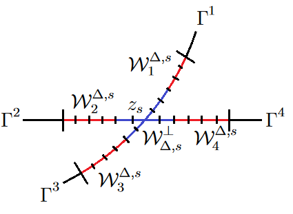
ℬ~j:𝒲1,𝒲1⟂⊕𝒲2,…,𝒲i⟂⊕𝒲i+1,…,𝒲nc​u​t−1⟂⊕𝒲nc​u​t,𝒲nc​u​t⟂.\tilde{\mathcal{B}}_{j}:{\mathcal{W}}_{1},{\mathcal{W}}_{1}^{\perp}\oplus{\mathcal{W}}_{2},\dots,{\mathcal{W}}_{i}^{\perp}\oplus{\mathcal{W}}_{i+1},\dots,{\mathcal{W}}_{n_{cut}-1}^{\perp}\oplus{\mathcal{W}}_{n_{cut}},{\mathcal{W}}_{n_{cut}}^{\perp}.

See Figure 1 below.

Refer to caption
Figure 1: The formation of the new basis from the old. Note that the interval illustrates the spectrum of BB. Note nc​u​t=7n_{cut}=7.

Note the abuse of notation that we will use for the rest of the
section: 𝒲i⟂=ℬi⊖𝒲i{\mathcal{W}}_{i}^{\perp}={\mathcal{B}}_{i}\ominus{\mathcal{W}}_{i} and ℬi⟂=ℬ⊖ℬi{\mathcal{B}}_{i}^{\perp}={\mathcal{B}}\ominus{\mathcal{B}}_{i}.

For simplicity, set 𝒲0=𝒲0⟂=ℬ0=0{\mathcal{W}}_{0}={\mathcal{W}}_{0}^{\perp}={\mathcal{B}}_{0}=0 and 𝒲nc​u​t+1=𝒲nc​u​t+1⟂=ℬnc​u​t+1=0{\mathcal{W}}_{n_{cut}+1}={\mathcal{W}}_{n_{cut}+1}^{\perp}={\mathcal{B}}_{n_{cut}+1}=0 and Inc​u​t={1}I_{n_{cut}}=\{1\} so that for 0≤i≤nc​u​t0\leq i\leq n_{cut}, ℬ~i=𝒲i⟂⊕𝒲i+1⊂ℬi⊕ℬi+1\tilde{\mathcal{B}}_{i}={\mathcal{W}}_{i}^{\perp}\oplus{\mathcal{W}}_{i+1}\subset{\mathcal{B}}_{i}\oplus{\mathcal{B}}_{i+1}. Now, let B′B^{\prime} be the block identity operator which equals the right endpoint of IiI_{i} multiplied by the identity on ℬ~i⊂ℬi⊕ℬi+1\tilde{\mathcal{B}}_{i}\subset{\mathcal{B}}_{i}\oplus{\mathcal{B}}_{i+1}, 0≤i≤nc​u​t−10\leq i\leq n_{cut}-1. Because BB has eigenvalues in III_{I} on ℬI+1{\mathcal{B}}_{I+1}, we see that ‖B−B′‖≤2nc​u​t\|B-B^{\prime}\|\leq\frac{2}{n_{cut}}.

We now show that the ℬ~i\tilde{\mathcal{B}}_{i} are almost invariant subspaces for HH, where we let H′H^{\prime} be the pinching of HH along ℬ~i\tilde{\mathcal{B}}_{i} so then ‖H−H′‖≤2​ϵ2\|H-H^{\prime}\|\leq 2\epsilon_{2}. This amounts to showing that applying HH to any vector in 𝒲i{\mathcal{W}}_{i} remains in 𝒲i−1⟂⊕𝒲i{\mathcal{W}}_{i-1}^{\perp}\oplus{\mathcal{W}}_{i} except that very small amounts are permitted to “leak out”. A similar statement would hold for 𝒲i−1⟂{\mathcal{W}}_{i-1}^{\perp}. The idea is that applying HH to 𝒲i⊂ℬi{\mathcal{W}}_{i}\subset{\mathcal{B}}_{i} can only make 𝒲i{\mathcal{W}}_{i} leak out into 𝒱1i+1{\mathcal{V}}_{1}^{i+1} and 𝒱Li−1{\mathcal{V}}_{L}^{i-1} through 𝒱Li{\mathcal{V}}_{L}^{i} and 𝒱1i{\mathcal{V}}_{1}^{i}, respectively. In details, let ℬi{\mathcal{B}}_{i} be written as the orthogonal direct sum of 𝒱1i,…,𝒱Li{\mathcal{V}}_{1}^{i},\dots,{\mathcal{V}}_{L}^{i} as in the statement of Lemma 2.

Recall that by Item 2, ‖P𝒲i⟂​H​P𝒲i‖≤ϵ2.\|P_{{\mathcal{W}}_{i}^{\perp}}HP_{{\mathcal{W}}_{i}}\|\leq\epsilon_{2}. By the block tridiagonality of HH, Pℬi⟂​H​P𝒲i=Pℬi⟂​H​(P𝒱1i+P𝒱Li)​P𝒲iP_{{\mathcal{B}}_{i}^{\perp}}HP_{{\mathcal{W}}_{i}}=P_{{\mathcal{B}}_{i}^{\perp}}H(P_{{\mathcal{V}}_{1}^{i}}+P_{{\mathcal{V}}_{L}^{i}})P_{{\mathcal{W}}_{i}}. Now, P𝒱Li​P𝒲i=0P_{{\mathcal{V}}_{L}^{i}}P_{{\mathcal{W}}_{i}}=0 and Pℬi⟂​H​P𝒱1i​P𝒲i=Pℬi⟂​H​P𝒱1iP_{{\mathcal{B}}_{i}^{\perp}}HP_{{\mathcal{V}}_{1}^{i}}P_{{\mathcal{W}}_{i}}=P_{{\mathcal{B}}_{i}^{\perp}}HP_{{\mathcal{V}}_{1}^{i}} maps into 𝒱Li−1⊂𝒲i−1⟂{\mathcal{V}}_{L}^{i-1}\subset\mathcal{W}_{i-1}^{\perp} so Pℬi⟂​H​P𝒲i=P𝒱Li−1​H​P𝒲i=P𝒲i−1⟂​H​P𝒲iP_{{\mathcal{B}}_{i}^{\perp}}HP_{{\mathcal{W}}_{i}}=P_{{\mathcal{V}}_{L}^{i-1}}HP_{{\mathcal{W}}_{i}}=P_{{\mathcal{W}}_{i-1}^{\perp}}HP_{{\mathcal{W}}_{i}}. Hence,

∥(1−Pℬ~i−1)\displaystyle\|(1-P_{\tilde{\mathcal{B}}_{i-1}}) H​Pℬ~i−1​P𝒲i|=‖H​P𝒲i−P𝒲i​H​P𝒲i−P𝒲i−1⟂​H​P𝒲i‖\displaystyle HP_{\tilde{\mathcal{B}}_{i-1}}P_{\mathcal{W}_{i}}\|=\|HP_{{\mathcal{W}}_{i}}-P_{{\mathcal{W}}_{i}}HP_{{\mathcal{W}}_{i}}-P_{{\mathcal{W}}_{i-1}^{\perp}}HP_{{\mathcal{W}}_{i}}\|
≤‖Pℬi​H​P𝒲i−P𝒲i​H​P𝒲i‖+‖Pℬi⟂​H​P𝒲i−P𝒲i−1⟂​H​P𝒲i‖≤ϵ2+0.\displaystyle\leq\|P_{{\mathcal{B}}_{i}}HP_{{\mathcal{W}}_{i}}-P_{{\mathcal{W}}_{i}}HP_{{\mathcal{W}}_{i}}\|+\|P_{{\mathcal{B}}_{i}^{\perp}}HP_{{\mathcal{W}}_{i}}-P_{{\mathcal{W}}_{i-1}^{\perp}}HP_{{\mathcal{W}}_{i}}\|\leq\epsilon_{2}+0.

Likewise, by taking adjoints, ‖P𝒲i​H​P𝒲i⟂‖≤ϵ2\|P_{\mathcal{W}_{i}}HP_{{\mathcal{W}}_{i}^{\perp}}\|\leq\epsilon_{2}. By the block triangularity of HH, Pℬi⟂​H​P𝒲i⟂=Pℬi⟂​H​(P𝒱1i+P𝒱Li)​P𝒲i⟂P_{{\mathcal{B}}_{i}^{\perp}}HP_{{\mathcal{W}}_{i}^{\perp}}=P_{{\mathcal{B}}_{i}^{\perp}}H(P_{{\mathcal{V}}_{1}^{i}}+P_{{\mathcal{V}}_{L}^{i}})P_{{\mathcal{W}}_{i}^{\perp}}. Now, P𝒱1i​P𝒲i⟂=0P_{{\mathcal{V}}_{1}^{i}}P_{{\mathcal{W}}_{i}^{\perp}}=0 and Pℬi⟂​H​P𝒱Li​P𝒲i⟂=Pℬi⟂​H​P𝒱LiP_{{\mathcal{B}}_{i}^{\perp}}HP_{{\mathcal{V}}_{L}^{i}}P_{{\mathcal{W}}_{i}^{\perp}}=P_{{\mathcal{B}}_{i}^{\perp}}HP_{{\mathcal{V}}_{L}^{i}} maps into 𝒱1i+1⊂𝒲i+1\mathcal{V}_{1}^{i+1}\subset\mathcal{W}_{i+1}, so Pℬi⟂​H​P𝒲i⟂=P𝒱1i+1​H​P𝒲i⟂=P𝒲i+1​H​P𝒲i⟂P_{{\mathcal{B}}_{i}^{\perp}}HP_{{\mathcal{W}}_{i}^{\perp}}=P_{{\mathcal{V}}_{1}^{i+1}}HP_{{\mathcal{W}}_{i}^{\perp}}=P_{{\mathcal{W}}_{i+1}}HP_{{\mathcal{W}}_{i}^{\perp}}. Hence,

∥(1−Pℬ~i)\displaystyle\|(1-P_{\tilde{\mathcal{B}}_{i}}) H​Pℬ~i​P𝒲i⟂|=‖H​P𝒲i⟂−P𝒲i+1​H​P𝒲i⟂−P𝒲i⟂​H​P𝒲i⟂‖\displaystyle HP_{\tilde{\mathcal{B}}_{i}}P_{{\mathcal{W}}_{i}^{\perp}}\|=\|HP_{{\mathcal{W}}_{i}^{\perp}}-P_{{\mathcal{W}}_{i+1}}HP_{{\mathcal{W}}_{i}^{\perp}}-P_{{\mathcal{W}}_{i}^{\perp}}HP_{{\mathcal{W}}_{i}^{\perp}}\|
≤‖Pℬi⟂​H​P𝒲i⟂−P𝒲i+1​H​P𝒲i⟂‖+‖Pℬi​H​P𝒲i⟂−P𝒲i⟂​H​P𝒲i⟂‖≤0+ϵ2.\displaystyle\leq\|P_{{\mathcal{B}}_{i}^{\perp}}HP_{{\mathcal{W}}_{i}^{\perp}}-P_{{\mathcal{W}}_{i+1}}HP_{{\mathcal{W}}_{i}^{\perp}}\|+\|P_{{\mathcal{B}}_{i}}HP_{{\mathcal{W}}_{i}^{\perp}}-P_{{\mathcal{W}}_{i}^{\perp}}HP_{{\mathcal{W}}_{i}^{\perp}}\|\leq 0+\epsilon_{2}.

So, it follows that

‖Pℬ~j⟂​H​Pℬ~j‖≤2​ϵ2.\|P_{\tilde{\mathcal{B}}_{j}}^{\perp}HP_{\tilde{\mathcal{B}}_{j}}\|\leq 2\epsilon_{2}.

Set H′=∑jPℬ~j​H​Pℬ~jH^{\prime}=\sum_{j}P_{\tilde{\mathcal{B}}_{j}}HP_{\tilde{\mathcal{B}}_{j}}. Because the spaces ℬ~i\tilde{\mathcal{B}}_{i} are orthogonal, we see that ‖H−H′‖≤2​ϵ2\|H-H^{\prime}\|\leq 2\epsilon_{2}. By construction B′B^{\prime} and H′H^{\prime} commute and we conclude.

7 Estimates, Putting it all Together

In this section we explore how the various constants discussed previously can be chosen to get the best possible decay in Lin’s theorem. There are cases where one might not want the best possible estimates, because perhaps picking a different rate allows one to not use Lemma 6.1 but instead use a different construction such as that of [47].

We now summarize the steps taken thus far in the construction, assuming a solution of Lemma 6.1 with exponent γ2=min⁡(γ3,γ4)\gamma_{2}=\min(\gamma_{3},\gamma_{4}). From A,BA,B self-adjoint with ‖A‖,‖B‖≤1\|A\|,\|B\|\leq 1, ‖[A,B]‖≤δ\|[A,B]\|\leq\delta we get (by applying Lemma 5.1) HH such that ‖H‖≤1,‖[H,B]‖≤C​o​n​s​t.δ\|H\|\leq 1,\|[H,B]\|\leq Const.\delta, and ‖A−H‖≤C​o​n​s​t.δ/Δ\|A-H\|\leq Const.\delta/\Delta. We get [H′,B′]=0[H^{\prime},B^{\prime}]=0 with ‖B−B′‖≤2/nc​u​t∼2​Δγ1\|B-B^{\prime}\|\leq 2/n_{cut}\sim 2\Delta^{\gamma_{1}} for 0<γ1<10<\gamma_{1}<1 and ‖H−H′‖≤2​ϵ2≤2​L−γ2​E​(1L)\|H-H^{\prime}\|\leq 2\epsilon_{2}\leq 2L^{-\gamma_{2}}E(\frac{1}{L}), where L∼2nc​u​t​Δ∼2​Δγ1−1L\sim\frac{2}{n_{cut}\Delta}\sim 2\Delta^{\gamma_{1}-1}. So, writing Δ=δγ0\Delta=\delta^{\gamma_{0}}, 0<γ0<10<\gamma_{0}<1, we get 2​L−1∼Δ1−γ1=δγ0​(1−γ1)2L^{-1}\sim\Delta^{1-\gamma_{1}}=\delta^{\gamma_{0}(1-\gamma_{1})} hence

‖A−H′‖≤C​o​n​s​t.δ/Δ+2​ϵ2≤C​o​n​s​t.δ1−γ0+δγ0​(1−γ1)​γ2​E​(δ−1)\displaystyle\|A-H^{\prime}\|\leq Const.\delta/\Delta+2\epsilon_{2}\leq Const.\delta^{1-\gamma_{0}}+\delta^{\gamma_{0}(1-\gamma_{1})\gamma_{2}}E(\delta^{-1}) (8)

and

‖B−B′‖≤2/nc​u​t≤C​o​n​s​t.δγ0​γ1.\displaystyle\|B-B^{\prime}\|\leq 2/n_{cut}\leq Const.\delta^{\gamma_{0}\gamma_{1}}. (9)

We want to minimize these, noting that γ2\gamma_{2}, which comes from Lemma 2, is the only constant that we cannot choose. Setting the three exponents equal we get γ0=11+γ1\gamma_{0}=\frac{1}{1+\gamma_{1}} and γ1=γ21+γ2\gamma_{1}=\frac{\gamma_{2}}{1+\gamma_{2}}, so the common value of the exponents will be chosen to be γ=γ21+2​γ2\gamma=\frac{\gamma_{2}}{1+2\gamma_{2}}. Because the value of γ2\gamma_{2} that we obtain is γ2=1/4\gamma_{2}=1/4, we obtain γ=1/6\gamma=1/6.

Note that this method cannot give the optimal exponent of γ=12\gamma=\frac{1}{2} (only potentially 12+ϵ\frac{1}{2}+\epsilon if we are allowed to take γ2\gamma_{2} arbitrarily large). This is partly because of the averaging that we do to make HH “finite range” as expressed in the title of Section II.A of [29], as a consequence of the δ/Δ\delta/\Delta factor.

If we were able to remove that factor (by improving the result or starting in a special case of AA) then we would then have to compare γ0​(1−γ1)​γ2\gamma_{0}(1-\gamma_{1})\gamma_{2} with γ0​γ1\gamma_{0}\gamma_{1} which gives γ1=γ21+γ2\gamma_{1}=\frac{\gamma_{2}}{1+\gamma_{2}}. Because we need to have AA finite range of distance Δ\Delta with respect to BB, we see that ‖[A,B]‖≤C​o​n​s​t.Δ\|[A,B]\|\leq Const.\Delta. This gives δ≤C​o​n​s​t.δγ0\delta\leq Const.\delta^{\gamma_{0}} so 0<γ0≤10<\gamma_{0}\leq 1. Because we do not need to worry about bounding A−HA-H (because we are starting with A=HA=H) we get

‖A−H′‖≤δγ0​(1−γ1)​γ2​E0​(1/δ)\displaystyle\|A-H^{\prime}\|\leq\delta^{\gamma_{0}(1-\gamma_{1})\gamma_{2}}E_{0}(1/\delta) (10)

and

‖B−B′‖≤2​δγ0​γ1.\displaystyle\|B-B^{\prime}\|\leq 2\delta^{\gamma_{0}\gamma_{1}}. (11)

So, we see that the rate we get is γ=γ21+γ2\gamma=\frac{\gamma_{2}}{1+\gamma_{2}}, which is an improvement. The value of γ2\gamma_{2} is 11 to then get the optimal exponent γ=1/2\gamma=1/2.

Note that Davidson in the proof of the equivalence of (QQ) and (Q′Q^{\prime}) showed that Lin’s theorem implies that we can pick γ2=1/2\gamma_{2}=1/2, which is an estimate that gives Lin’s theorem with γ=1/4\gamma=1/4.

8 General Approach to the construction of 𝒲\mathcal{W}.

In this section we define subspaces 𝒳~i\tilde{\mathcal{X}}_{i} and 𝒳~i′\tilde{\mathcal{X}}_{i}^{\prime} to describe the motivating ideas used in [47]. We then define smooth cut off functions ℱω0r,w​(t)\mathcal{F}^{r,w}_{\omega_{0}}(t) and use them to define the spaces 𝒳i\mathcal{X}_{i}, which will be put together in some sense to define 𝒲\mathcal{W} following [29].

Because we need to essentially recover 𝒱1\mathcal{V}_{1} as a subspace of 𝒲\mathcal{W} by Item 1, we might consider finding subspaces 𝒳~i\tilde{\mathcal{X}}_{i} such that 𝒱1\mathcal{V}_{1} is approximately a subset of the sum of the 𝒳i~\tilde{\mathcal{X}_{i}}. For example, consider breaking up [−1,1][-1,1] into nw​i​nn_{win} many disjoint intervals IiI_{i} similarly to how we did before then we could consider 𝒳~i=[χIi​(J)]​(𝒱1)\tilde{\mathcal{X}}_{i}=[\chi_{I_{i}}(J)](\mathcal{V}_{1}). This space recovers 𝒱1\mathcal{V}_{1} because any element vv in 𝒱1\mathcal{V}_{1} can be written v=∑ixiv=\sum_{i}x_{i}, where xi=χIi​(J)​vx_{i}=\chi_{I_{i}}(J)v.

These spaces are almost invariant: Let ω⁡(i)\omega(i) be the midpoint of IiI_{i} and x∈𝒳~ix\in\tilde{\mathcal{X}}_{i}. We have that

|(J−ω⁡(i))​x|=|(J−ω⁡(i))​χIi​(J)​x|≤‖(J−ω⁡(i))​χIi​(J)‖|x|≤|Ii|2​|x|.\displaystyle|(J-\omega(i))x|=|(J-\omega(i))\chi_{I_{i}}(J)x|\leq\|(J-\omega(i))\chi_{I_{i}}(J)\||x|\leq\frac{|I_{i}|}{2}|x|. (12)

This shows that J​xJx is almost in span⁡(x)⊂𝒳~i\operatorname{span}(x)\subset\tilde{\mathcal{X}}_{i}, where the error depends on the norm of xx. Also, these spaces 𝒳~i\tilde{\mathcal{X}}_{i} are also orthogonal, so we obtain that if v=∑ixiv=\sum_{i}x_{i} then |v|2=∑i|xi|2|v|^{2}=\sum_{i}|x_{i}|^{2}.

Putting all of this together, if we set 𝒲~=⨁i𝒳~i\tilde{\mathcal{W}}=\bigoplus_{i}\tilde{\mathcal{X}}_{i}, we have Item 1 because it contains 𝒱1\mathcal{V}_{1}. It satisfies Item 2 because if w∈𝒲~w\in\tilde{\mathcal{W}} then we can write it as w=∑ixiw=\sum_{i}x_{i}, xi∈𝒳~ix_{i}\in\tilde{\mathcal{X}}_{i}. Because the IiI_{i} are disjoint,

|J​w−∑iω⁡(i)​xi|2\displaystyle|Jw-\sum_{i}\omega(i)x_{i}|^{2} =|∑i(J−ω⁡(i))​xi|2=∑i|(J−ω⁡(i))​xi|2\displaystyle=|\sum_{i}(J-\omega(i))x_{i}|^{2}=\sum_{i}|(J-\omega(i))x_{i}|^{2}
≤∑i(|Ii|2)2​|xi|2=(|Ii|2)2​|w|2.\displaystyle\leq\sum_{i}\left(\frac{|I_{i}|}{2}\right)^{2}|x_{i}|^{2}=\left(\frac{|I_{i}|}{2}\right)^{2}|w|^{2}. (13)

So because xi∈𝒲~x_{i}\in\tilde{\mathcal{W}},

|P𝒲~⟂​J​w|=|P𝒲~⟂​(J​w−∑iω⁡(i)​xi)|≤|Ii|2​|w|.\displaystyle|P_{\tilde{\mathcal{W}}^{\perp}}Jw|=|P_{\tilde{\mathcal{W}}^{\perp}}\left(Jw-\sum_{i}\omega(i)x_{i}\right)|\leq\frac{|I_{i}|}{2}|w|. (14)

This general set-up is common ground for Szarek’s and Hastings’ arguments. They differ in how to modify this core argument to get a result concerning Item 3. We proceed with a modification used in both constructions.

We want to show that Item 3 holds as well for 𝒲~\tilde{\mathcal{W}}, but it might not unless we address an issue. Recall that 𝒳~i={χIi​(J)​v:v∈𝒱1}\tilde{\mathcal{X}}_{i}=\{\chi_{I_{i}}(J)v:v\in\mathcal{V}_{1}\}. Let S1S_{1} be a matrix whose columns are a fixed orthonormal basis of 𝒱1\mathcal{V}_{1}, where d=dim𝒱1d=\dim\mathcal{V}_{1}. Then S1S_{1} is an isometric isomorphism between ℂd\mathbb{C}^{d} and 𝒱1\mathcal{V}_{1} and R⁡(χIi​(J)​S1)=𝒳~iR(\chi_{I_{i}}(J)S_{1})=\mathcal{\tilde{X}}_{i}.

We might hope that we have exponential decay of the columns of S1S_{1} (which would provide what we want) along the lines of Remark 3.3. This might not happen. To see this, [29] gives an example of an n×nn\times n matrix of the form:

(01/401/401/4001/401/4001/401/4⋱01/4⋱⋱0⋱⋱01/401/41/2)\begin{pmatrix}0&1/4&0&&\\ 1/4&0&1/4&0&\\ 0&1/4&0&1/4&0\\ &0&1/4&0&1/4&\ddots\\ &&0&1/4&\ddots&\ddots&0\\ &&&\ddots&\ddots&0&1/4\\ &&&&0&1/4&1/2\\ \end{pmatrix}

Here, we can take 𝒱1\mathcal{V}_{1} to be the first basis vector. For nn large, its spectrum is distributed finely in [−1/2,1/2][-1/2,1/2] with a single (with multiplicity one) eigenvalue at around 5/85/8.

For example, MATLAB calculations give that if S1S_{1} is just the first standard basis vector then χ[5/8−1/100,5/8+1/100]​(J)​S1\chi_{[5/8-1/100,5/8+1/100]}(J)S_{1} is, for n=10n=10,

10−3×(0.0016,0.0040,0.0084,0.0171,0.0343,0.0686,0.1373,0.2747,0.5493,1.0987)T,10^{-3}\times(0.0016,0.0040,0.0084,0.0171,0.0343,0.0686,0.1373,0.2747,0.5493,1.0987)^{T},

and for n=50n=50

10−15×(CLOSE\displaystyle 10^{-15}\times( 0.0000,…,0.0000,0.0001,0.0002,0.0005,0.001,0.002,0.004,0.008,0.016,\displaystyle 0.0000,\dots,0.0000,0.0001,0.0002,0.0005,0.001,0.002,0.004,0.008,0.016,
OPEN0.031,0.062,0.125,0.251,0.502,1.004)T.\displaystyle 0.031,0.062,0.125,0.251,0.502,1.004)^{T}.

The pattern is that the norm of this vector is very small, but does not have small projection onto 𝒱L\mathcal{V}_{L} relative to its norm. One way of addressing this phenomenon is to disallow vectors that have too small norm, by removing columns of χIi​(J)​S\chi_{I_{i}}(J)S that are too small. However, that does not exclude the case that all of its columns are large, but a linear combination of them are of this problematic type. For example, we might have chosen a different basis for 𝒱1\mathcal{V}_{1}. If one modifies the operators χIi​(J)​S\chi_{I_{i}}(J)S so that we still maintain Item 1 and Item 2 and removing the issue discussed above, we might be closer to showing Item 3.

The approach to this problem is to write τ~i=χIi​(J)​S1\tilde{\tau}_{i}=\chi_{I_{i}}(J)S_{1} and remove its singular values that are too small by letting Z~i\tilde{Z}_{i} project onto the eigenspace of τ~i∗​τ~i{\tilde{\tau}_{i}}^{\ast}\tilde{\tau}_{i} for eigenvalues less than some λm​i​n\lambda_{min}. Then define new spaces 𝒳~i′\tilde{\mathcal{X}}_{i}^{\prime} to be the range of τ~i​(1−Z~i)\tilde{\tau}_{i}(1-\tilde{Z}_{i}) and let 𝒲~′=⨁i𝒳~i′\tilde{\mathcal{W}}^{\prime}=\bigoplus_{i}\tilde{\mathcal{X}}_{i}^{\prime}, an orthogonal direct sum.

Now, this definition of 𝒳~i′\tilde{\mathcal{X}}_{i}^{\prime} gives that for any x∈𝒳~i′x\in\tilde{\mathcal{X}}_{i}^{\prime}, we have some x∈ℂd\textbf{x}\in\mathbb{C}^{d} such that τ~i​(1−Z~i)​x=x\tilde{\tau}_{i}(1-\tilde{Z}_{i})\textbf{x}=x and we can choose x to be in the range of 1−Z~i1-\tilde{Z}_{i} so that τ~i​x=x\tilde{\tau}_{i}\textbf{x}=x. We call x the representative of xx (by τ~i\tilde{\tau}_{i}). Writing x=∑axa\textbf{x}=\sum_{a}\textbf{x}^{a} as the orthogonal sum of eigenvectors xa\textbf{x}^{a} of τ~i∗​τ~i{\tilde{\tau}_{i}}^{\ast}\tilde{\tau}_{i} with eigenvalues λa≥λm​i​n\lambda_{a}\geq\lambda_{min} we obtain

|τ~i​x|2=∑a,b(τ~i​xa,τi~​xb)=∑a(τi~∗​τ~i​xa,xa)≥∑aλm​i​n​|xa|2,|\tilde{\tau}_{i}\textbf{x}|^{2}=\sum_{a,b}(\tilde{\tau}_{i}\textbf{x}^{a},\tilde{\tau_{i}}\textbf{x}^{b})=\sum_{a}(\tilde{\tau_{i}}^{\ast}\tilde{\tau}_{i}\textbf{x}^{a},\textbf{x}^{a})\geq\sum_{a}\lambda_{min}|\textbf{x}^{a}|^{2},

so

|τ~i​x|≥λm​i​n1/2​|x|.|\tilde{\tau}_{i}\textbf{x}|\geq\lambda_{min}^{1/2}|\textbf{x}|.

This guarantees that we do not have any exponentially small “problematic” vectors if we make λm​i​n\lambda_{min} go to zero only like a power of LL. This adjustment seemingly does not offer a way to prove Item 3, however, if it is now true.

Item 1 holds for 𝒲~′\tilde{\mathcal{W}}^{\prime} because for any v∈𝒱1v\in\mathcal{V}_{1}, we can write it as the orthogonal direct sum ∑ixi\sum_{i}x_{i}, where xi=χIi​(J)​v=τ~i​xx_{i}=\chi_{I_{i}}(J)v=\tilde{\tau}_{i}\textbf{x} and v=S​xv=S\textbf{x}. Then we get that

|τ~i​x−τ~i​(1−Z~i)​x|2=|τ~i​Z~i​x|2≤λm​i​n​|x|2=λm​i​n​|v|2.|\tilde{\tau}_{i}\textbf{x}-\tilde{\tau}_{i}(1-\tilde{Z}_{i})\textbf{x}|^{2}=|\tilde{\tau}_{i}\tilde{Z}_{i}\textbf{x}|^{2}\leq\lambda_{min}|\textbf{x}|^{2}=\lambda_{min}|v|^{2}.

Because the ranges of the τ~i\tilde{\tau}_{i} are orthogonal, we get that

|P𝒲~′⁣⟂​v|\displaystyle|P_{\tilde{\mathcal{W}}^{\prime\perp}}v| ≤|∑iτ~i​x−∑iτ~i​(1−Z~i)​x|=|∑iτ~i​Z~i​x|=(∑i=0nw​i​n−1|τ~i​Z~i​x|2)1/2\displaystyle\leq|\sum_{i}\tilde{\tau}_{i}\textbf{x}-\sum_{i}\tilde{\tau}_{i}(1-\tilde{Z}_{i})\textbf{x}|=|\sum_{i}\tilde{\tau}_{i}\tilde{Z}_{i}\textbf{x}|=\left(\sum_{i=0}^{n_{win}-1}|\tilde{\tau}_{i}\tilde{Z}_{i}\textbf{x}|^{2}\right)^{1/2}
≤(nw​i​n​λm​i​n)1/2​|v|.\displaystyle\leq(n_{win}\lambda_{min})^{1/2}|v|.

We see that Item 2 holds as follows. Let ω⁡(i)\omega(i) be the midpoint of the interval IiI_{i}. For w=∑ixiw=\sum_{i}x_{i} with xi∈𝒳~i′x_{i}\in\tilde{\mathcal{X}}_{i}^{\prime} so χIi​(J)​xi=xi\chi_{I_{i}}(J)x_{i}=x_{i}, we have

|(J−ω⁡(i))​xi|≤|Ii|2​|xi|.|(J-\omega(i))x_{i}|\leq\frac{|I_{i}|}{2}|x_{i}|.

Recall that xi∈𝒳~i′⊂𝒳~ix_{i}\in\tilde{\mathcal{X}}^{\prime}_{i}\subset\tilde{\mathcal{X}}_{i} and J​xi∈𝒳~iJx_{i}\in\tilde{\mathcal{X}}_{i}. So, because the 𝒳~i\tilde{\mathcal{X}}_{i} are orthogonal we obtain

|PW~′⁣⟂​J​w|2\displaystyle|P_{\tilde{W}^{\prime\perp}}Jw|^{2} =|P𝒲~′⁣⟂​∑i(J−ω⁡(i))​xi|2≤|∑i(J−ω⁡(i))​xi|2=∑i|(J−ω⁡(i))​xi|2\displaystyle=|P_{\tilde{\mathcal{W}}^{\prime\perp}}\sum_{i}(J-\omega(i))x_{i}|^{2}\leq|\sum_{i}(J-\omega(i))x_{i}|^{2}=\sum_{i}|(J-\omega(i))x_{i}|^{2}
≤∑i(|Ii|2​|xi|)2=(|Ii|2​|w|)2\displaystyle\leq\sum_{i}\left(\frac{|I_{i}|}{2}|x_{i}|\right)^{2}=\left(\frac{|I_{i}|}{2}|w|\right)^{2}

so |P𝒲~′⁣⟂​J​w|≤|Ii|2​|w||P_{\tilde{\mathcal{W}}^{\prime\perp}}Jw|\leq\frac{|I_{i}|}{2}|w|.

An important property that we used in approximating J​wJw was that J​w=∑iJ​xiJw=\sum_{i}Jx_{i} and not only is ∑xi=w\sum x_{i}=w an orthogonal decomposition but the (J−ω⁡(i))​xi(J-\omega(i))x_{i} are also orthogonal because the τi\tau_{i} are. Later when we define 𝒳i\mathcal{X}_{i} to be a subspace of the range of ℱω⁡(i)0,κ​(J){\mathcal{F}}^{0,\kappa}_{\omega(i)}(J) (where ℱω⁡(i)0,κ{\mathcal{F}}^{0,\kappa}_{\omega(i)} are smooth overlapping cut-off functions), we see that J⁡(𝒳i)J(\mathcal{X}_{i}) are nonconsecutively orthogonal. One could see that the above argument would work, except that we seemingly do not have

∑i|xi|2≤C​o​n​s​t.|w|2.\displaystyle\sum_{i}|x_{i}|^{2}\leq Const.|w|^{2}. (15)

These are some of the issues that Hastings deals with using the ℱω⁡(i)0,κ{\mathcal{F}}^{0,\kappa}_{\omega(i)}. The subspaces that we obtain will no longer be orthogonal (which causes its own issues), but in Lemma 14.2.1 we obtain the estimate

∑i|xi|2≤C​o​n​s​t.lb​|w|2\sum_{i}|x_{i}|^{2}\leq Const.l_{b}|w|^{2}

where lbl_{b} grows like a power of LL and along with the decay given in Corollary 5.7 we can obtain the third property. The smoothness of ℱω⁡(i)0,κ{\mathcal{F}}^{0,\kappa}_{\omega(i)} ensures the sufficient decay of its Fourier transform and hence that of Corollary 5.7. As stated in [29], “The smoothness will be essential to ensure that the vectors … have most of their amplitude in the first blocks rather than the last blocks”.

9 Dimensional-Dependent Results

In this section we describe the dimensional dependent results prior to [29] which indicate the necessity of both matrices being self-adjoint and why it is necessary that the proof of Lin’s theorem involve the structure of both almost commuting matrices. This section can be skipped if reading for the proof of Hastings’ result.

One comment is that Lin’s theorem is essentially the mm dimensional case if we assume that AA always has at most mm distinct eigenvalues. More precisely, Pearcy and Shields’ argument in [41] indicates that if AA is self-adjoint and has at most mm distinct eigenvalues, then there are commuting matrices A′,B′A^{\prime},B^{\prime} where A′A^{\prime} is self-adjoint, B′B^{\prime} is self-adjoint if BB is, and

‖A−A′‖,‖B−B′‖≤(m−12​‖[A,B]‖)1/2.\|A-A^{\prime}\|,\|B-B^{\prime}\|\leq\left(\frac{m-1}{2}\|[A,B]\|\right)^{1/2}.

This allows us to choose δ=2m−1​ϵ2\delta=\frac{2}{m-1}\epsilon^{2}. The ideas in Pearcy and Shields’ argument are illustrated in the following cheap result.

Proposition 9.1.

Let A,B∈Mn​(ℂ)A,B\in M_{n}(\mathbb{C}), where AA is self-adjoint with at most mm distinct eigenvalues. Then there are commuting A′,B′A^{\prime},B^{\prime} such that A′A^{\prime} is self-adjoint and

‖A−A′‖,‖B−B′‖≤m2​‖[A,B]‖1/2.\|A-A^{\prime}\|,\|B-B^{\prime}\|\leq\frac{m}{\sqrt{2}}\|[A,B]\|^{1/2}.
Proof.

We partition the spectrum of AA into intervals IiI_{i} of length at most cm​δ1/2c_{m}\delta^{1/2}, where δ:=‖[A,B]‖\delta:=\|[A,B]\|. We choose cmc_{m} later so as to make our bound for ‖A−A′‖\|A-A^{\prime}\| equal to that of ‖B−B′‖\|B-B^{\prime}\|. We write AA as block multiples of the identity (ai​Ii)(a_{i}I_{i}), with the aia_{i} ordered increasingly, and BB as a block matrix (Bi​j)(B_{ij}), so then [A,B]r​s=(ar−as)​Br​s[A,B]_{rs}=(a_{r}-a_{s})B_{rs}.

We cannot avoid that some off-diagonal terms of (Bi​j)(B_{ij}) might not be small where the eigenvalues of AA are close because of behavior depicted in Example 4.5. A way of dealing with this is to use the trick in Hastings’ proof of the tridiagonal case and merge together intervals that are too close. This will be doable, because our estimate will depend on the number of eigenvalues.

Doing this, take our partition of half-open intervals IiI_{i} of length cm​δ1/2c_{m}\delta^{1/2} and discard the intervals that do not intersect the spectrum of AA to obtain half-open intervals IjI_{j}. Merge together neighboring intervals to obtain merged intervals I~k\tilde{I}_{k}. Because there were at most mm eigenvalues, these merged intervals have length at most m​cm​δ1/2mc_{m}\delta^{1/2} and there is a gap of at least cm​δ1/2c_{m}\delta^{1/2} (the length of one IiI_{i}). We let A′A^{\prime} be the block matrix formed by merging the diagonal entries of AA that correspond to the merged intervals and replacing the entries with the midpoint of the merged interval. Then ‖A−A′‖≤12​m​cm​δ1/2\|A-A^{\prime}\|\leq\frac{1}{2}mc_{m}\delta^{1/2}. We let B′B^{\prime} be the matrix gotten by discarding the off-diagonal blocks Br​sB_{rs} where ara_{r} and asa_{s} are from different merged blocks. Because |ar−as|​‖Br​s‖≤‖[A,B]‖=δ|a_{r}-a_{s}|\|B_{rs}\|\leq\|[A,B]\|=\delta and for ar,asa_{r},a_{s} from different merged blocks, |ar−as|≥cm​δ1/2|a_{r}-a_{s}|\geq c_{m}\delta^{1/2} so we obtain for these r,sr,s, ‖Br​s‖≤1cm​δ1/2\|B_{rs}\|\leq\frac{1}{c_{m}}\delta^{1/2}.

Because matrices in Mn​(ℂ)M_{n}(\mathbb{C}) are being expressed as square block matrices with at most mm rows, ‖B−B′‖≤mcm​δ1/2\|B-B^{\prime}\|\leq\frac{m}{c_{m}}\delta^{1/2}. Setting cm=2c_{m}=\sqrt{2}, we obtain

‖A−A′‖,‖B−B′‖≤m2​δ1/2.\|A-A^{\prime}\|,\|B-B^{\prime}\|\leq\frac{m}{\sqrt{2}}\delta^{1/2}.

∎

Remark 9.2.

Davidson’s counter-example in [14] of (n2+1)×(n2+1)(n^{2}+1)\times(n^{2}+1) self-adjoint AnA_{n} and nearly normal BnB_{n} that satisfy ‖[An,Bn]‖=1/n2\|[A_{n},B_{n}]\|=1/n^{2} with bounded norms without being nearby commuting matrices An′,Bn′A_{n}^{\prime},B_{n}^{\prime} where An′A_{n}^{\prime} is self-adjoint shows that [41]’s result is asymptotically optimal. Choi in [13] also has a similar counter-example showing that there are no nearby commuting matrices at all with the same asymptotic estimates.

The choice of the groupings of eigenvalues of AA in Pearcy and Shileds’ result does not involve BB in any way, besides the use of ‖[A,B]‖\|[A,B]\|. A difficulty in solving Lin’s theorem involves the fact that we need to use the structure of BB when constructing A′A^{\prime} (and vice-versa) unless ‖[A,B]‖\|[A,B]\| is very small. We explore these two ideas in the next two results.

Proposition 9.3.

Suppose that Ak,Bk∈Mnk​(ℂ)A_{k},B_{k}\in M_{n_{k}}(\mathbb{C}) are self-adjoint contractions. If
‖[Ak,Bk]‖→0\|[A_{k},B_{k}]\|\to 0, by Lin’s theorem there are self-adjoint, commuting Ak′,Bk′A_{k}^{\prime},B_{k}^{\prime} so that
‖Ak−Ak′‖,‖Bk−Bk′‖→0\|A_{k}-A_{k}^{\prime}\|,\|B_{k}-B_{k}^{\prime}\|\to 0. Let mkm_{k} be the number of eigenvalues of Ak′A_{k}^{\prime}.

If the choice of Ak′A_{k}^{\prime} can be made independent of BkB_{k}, then supkmk<∞\sup_{k}m_{k}<\infty.

Proof.

We prove this by contradiction. Choose a subsequence and relabel so that limkmk=∞\lim_{k}m_{k}=\infty.

By the Pigeonhole principle, there are two distinct eigenvalues λk1,λk2\lambda_{k}^{1},\lambda_{k}^{2} of Ak′A_{k}^{\prime} with eigenvectors vk1,vk2v_{k}^{1},v_{k}^{2}, respectively, so that |λk1−λk2|≤2/mk|\lambda_{k}^{1}-\lambda_{k}^{2}|\leq 2/m_{k}. If we define BkB_{k} to be the linear operator satisfying Bk​vk1=vk2,Bk​vk2=vk1B_{k}v_{k}^{1}=v_{k}^{2},B_{k}v_{k}^{2}=v_{k}^{1}, and is identically zero on the orthogonal complement of span⁡(vk1,vk2)\operatorname{span}(v_{k}^{1},v_{k}^{2}). Then ‖[Ak′,Bk]‖≤2/mk\|[A_{k}^{\prime},B_{k}]\|\leq 2/m_{k} so

‖[Ak,Bk]‖≤|Ak−Ak′|‖Bk‖+|[Ak′,Bk]|→0.\|[A_{k},B_{k}]\|\leq\|A_{k}-A_{k}^{\prime}\|\|B_{k}\|+\|[A_{k}^{\prime},B_{k}]\|\to 0.

If Bk′B_{k}^{\prime} is any matrix that commutes with Ak′A_{k}^{\prime} then the eigenspaces of Ak′A_{k}^{\prime} are invariant under Bk′B_{k}^{\prime}. This means that when writing Bk′B_{k}^{\prime} as a block diagonal matrix with respect to the eigenspaces of Ak′A_{k}^{\prime}, it must be diagonal. This shows that ‖Bk−Bk′‖≥1\|B_{k}-B_{k}^{\prime}\|\geq 1, which contradicts our assumption. ∎

The following result illustrates what seems to be a rather strict requirement on the size of the commutators because it destroys the invariants for three almost commuting Hermitians. Compare to Remark 9.2.

Corollary 9.4.

Let Ak,Bk,Ck∈Mnk​(ℂ)A_{k},B_{k},C_{k}\in M_{n_{k}}(\mathbb{C}) be self-adjoint contractions with AkA_{k} having mkm_{k} (distinct) eigenvalues. If ‖[Ak,Bk]‖,‖[Ak,Ck]‖=o⁡(1/mk)\|[A_{k},B_{k}]\|,\|[A_{k},C_{k}]\|=o(1/m_{k}) and ‖[Bk,Ck]‖=o⁡(1)\|[B_{k},C_{k}]\|=o(1) then there are self-adjoint commuting contractions Ak′,Bk′,Ck′A^{\prime}_{k},B^{\prime}_{k},C^{\prime}_{k} such that

‖Ak−Ak′‖,‖Bk−Bk′‖,‖Ck−Ck′‖=o⁡(1).\|A_{k}-A^{\prime}_{k}\|,\|B_{k}-B^{\prime}_{k}\|,\|C_{k}-C^{\prime}_{k}\|=o(1).
Proof.

Note that o⁡(1)o(1) only depends on kk. Without loss of generality, suppose that ‖[Ak,Ck]‖≤‖[Ak,Bk]‖\|[A_{k},C_{k}]\|\leq\|[A_{k},B_{k}]\|. Because the construction of Ak′A_{k}^{\prime} in [41] only uses BkB_{k} through a bound for ‖[Ak,Bk]‖\|[A_{k},B_{k}]\| and the construction of Bk′B_{k}^{\prime} is as below, we see that it works equally as well for CkC_{k}.

Applying [41]’s construction to Ak,BkA_{k},B_{k}, we get disjoint intervals I1k,…,IrkkI_{1}^{k},\dots,I_{r^{k}}^{k} that cover σ⁡(Ak)\sigma(A_{k}). For the projections Pik=EIik​(Ak)P_{i}^{k}=E_{I_{i}^{k}}(A_{k}), we can modify the spectrum of Aki:=Pik​Ak​PikA_{k}^{i}:=P_{i}^{k}A_{k}P_{i}^{k} to get multiples of identity matrices (A′k)i({A^{\prime}}_{k})^{i} which form the diagonal entries of the block diagonal matrix Ak′A^{\prime}_{k}. This construction satisfies the following properties:

‖Ak−Ak′‖≤(mk−12​‖[Ak,Bk]‖)1/2=:ϵk=o⁡(1).\|A_{k}-A_{k}^{\prime}\|\leq\left(\frac{m_{k}-1}{2}\|[A_{k},B_{k}]\|\right)^{1/2}=:\epsilon_{k}=o(1).

and for Bk′′=∑iPik​Bk​Pik,B_{k}^{\prime\prime}=\sum_{i}P_{i}^{k}B_{k}P_{i}^{k}, Ck′′=∑iPik​Ck​PikC_{k}^{\prime\prime}=\sum_{i}P_{i}^{k}C_{k}P_{i}^{k} we have ‖Bk−Bk′′‖,‖Ck−Ck′′‖≤ϵk=o⁡(1)\|B_{k}-B_{k}^{\prime\prime}\|,\|C_{k}-C_{k}^{\prime\prime}\|\leq\epsilon_{k}=o(1). Then

‖[Bk′′,Ck′′]‖≤‖[Bk,Ck]‖+2|Bk−Bk′′​‖+2‖​Ck−Ck′′|=o⁡(1).\|[B_{k}^{\prime\prime},C_{k}^{\prime\prime}]\|\leq\|[B_{k},C_{k}]\|+2\|B_{k}-B_{k}^{\prime\prime}\|+2\|C_{k}-C_{k}^{\prime\prime}\|=o(1).

By definition,

‖[Pik​Bk​Pik,Pik​Ck​Pik]‖=‖Pik​[Bk′′,Ck′′]​Pik‖=o⁡(1)\|[P_{i}^{k}B_{k}P_{i}^{k},P_{i}^{k}C_{k}P_{i}^{k}]\|=\|P_{i}^{k}[B_{k}^{\prime\prime},C_{k}^{\prime\prime}]P_{i}^{k}\|=o(1)

and so we can apply Lin’s theorem to these block matrices, so there are commuting self-adjoint contractions Bki,CkiB_{k}^{i},C_{k}^{i} of the same block size as Pik​Bk​Pik,Pik​Ck​PikP_{i}^{k}B_{k}P_{i}^{k},P_{i}^{k}C_{k}P_{i}^{k} such that ‖Bki−Pik​Bk​Pik‖,‖Cki−Pik​Ck​Pik‖=o⁡(1)\|B_{k}^{i}-P_{i}^{k}B_{k}P_{i}^{k}\|,\|C_{k}^{i}-P_{i}^{k}C_{k}P_{i}^{k}\|=o(1). Since Pik​Ak′​PikP_{i}^{k}A_{k}^{\prime}P_{i}^{k} is a multiple of the identity on R⁡(Pik)R(P_{i}^{k}), we see that forming Bk′=⨁iBki,Ck′=⨁iCkiB_{k}^{\prime}=\bigoplus_{i}B_{k}^{i},C_{k}^{\prime}=\bigoplus_{i}C_{k}^{i} gives us commuting self-adjoint matrices Ak′,Bk′,Ck′A_{k}^{\prime},B_{k}^{\prime},C_{k}^{\prime} satisfying the statement of the lemma. ∎

Before continuing with a discussion of Hastings’ approach to Lemma 6.4, we pause to discuss Szarek’s approach to this lemma. Szarek proves a dimensional-dependent version of this lemma in the following result from [47]. Note that this result is constructive and although is expressed in terms of Davidson’s third formulation of Lin’s theorem, it is readily transformed into the form that we have discussed in this paper.

Proposition 9.5.

Let JJ be self-adjoint with ‖J‖≤1\|J\|\leq 1 acting on ℬ{\mathcal{B}} with LL orthogonal subspaces 𝒱i{\mathcal{V}}_{i} with respect to which JJ is block tridiagonal. If for some i<Li<L we set m=dim𝒱im=\dim\mathcal{V}_{i}, then there is a subspace 𝒲\mathcal{W} such that 𝒱1⊂𝒲⟂𝒱L\mathcal{V}_{1}\subset\mathcal{W}\perp\mathcal{V}_{L} and

‖P𝒲⟂​J​P𝒲‖≤ϵ1​(L),\|P_{{\mathcal{W}}^{\perp}}JP_{\mathcal{W}}\|\leq\epsilon_{1}(L),

where ϵ1​(L)=C​o​n​s​t.(mL)1/9\displaystyle\epsilon_{1}(L)=Const.\left(\frac{m}{L}\right)^{1/9}.

Remark 9.6.

Szarek provides an argument that reduces the proof of the previous proposition to the case that all the 𝒱i\mathcal{V}_{i}, in particular, 𝒱1\mathcal{V}_{1} has dimension mm. This argument actually can be extended to say that not only can all the blocks of JJ be large, but we only need one off-diagonal block to have small rank and so can set m=rank⁡P𝒱i+1​J​P𝒱im=\operatorname{rank}P_{\mathcal{V}_{i+1}}JP_{\mathcal{V}_{i}}.

The point of this remark is that not does this result apply for a matrix JJ that contains blocks like these:

(∗11∗∗∗∗∗∗∗∗∗)\begin{pmatrix}\ast&1&&\\ 1&\ast&\ast&\ast\\ &\ast&\ast&\ast\\ &\ast&\ast&\ast\end{pmatrix}

because there is a diagonal block (corresponding to dim𝒱i\dim\mathcal{V}_{i}) of size one, but this result also applies if there are blocks like these (potentially under a change of basis for the subspaces 𝒱i\mathcal{V}_{i}):

(∗∗∗∗∗∗∗∗∗∗∗∗∗∗∗∗11∗∗∗∗∗∗∗∗∗).\begin{pmatrix}\ast&\ast&\ast&\ast&&&\\ \ast&\ast&\ast&\ast&&&\\ \ast&\ast&\ast&\ast&&&\\ \ast&\ast&\ast&\ast&1&&\\ &&&1&\ast&\ast&\ast\\ &&&&\ast&\ast&\ast\\ &&&&\ast&\ast&\ast\end{pmatrix}.

The argument in [47] involves using the general approach discussed in Section 8, however some modifications are made to obtain the last inequality. The construction involves several ideas. One of these ideas is that to obtain the approximate orthogonality of 𝒲\mathcal{W} and 𝒱L\mathcal{V}_{L}, Szarek forms 𝒲\mathcal{W} exactly as 𝒲~′\tilde{\mathcal{W}}^{\prime}, however the intervals IiI_{i} will not cover σ⁡(J)\sigma(J) but will be constructed by the application of the following lemma.

Lemma 9.7.

Let μ\mu be a finite positive measure on [0,1][0,1] and let κ>8​η>0\kappa>8\eta>0. Then there are disjoint intervals IiI_{i} for i=1,…,nw​i​ni=1,\dots,n_{win} such that

  1. 1.

    nw​i​n≤2κn_{win}\leq\displaystyle\frac{2}{\kappa}

  2. 2.

    |Ij|≤κ|I_{j}|\leq\kappa

  3. 3.

    dist⁡(Ii,Ij)≥η,i≠j\operatorname{dist}(I_{i},I_{j})\geq\eta,\,i\neq j

  4. 4.

    μ⁡([0,1]∖⋃jIj)≤4​ηκ​μ​([0,1])\mu\left([0,1]\setminus\bigcup_{j}I_{j}\right)\leq\displaystyle\frac{4\eta}{\kappa}\mu([0,1])

Based on what we did in the previous section, what remains is to show is that 𝒱1\mathcal{V}_{1} still belongs approximately to 𝒲\mathcal{W} and that 𝒲\mathcal{W} is approximately orthogonal to 𝒱L\mathcal{V}_{L}. The first statement follows from the construction of the intervals through the application of the last inequality in the interval lemma above. Because the construction of μ\mu is related to projection onto 𝒱1\mathcal{V}_{1}, the dimension mm of 𝒱1\mathcal{V}_{1} appears in the estimates as it is the trace of this projection.

The approximate orthogonality follows from the key observation that by using polynomial interpolation, there are polynomials pip_{i} such that 0≤pi≤10\leq p_{i}\leq 1, pi≈χIip_{i}\approx\chi_{I_{i}} on IiI_{i} and pi≈0p_{i}\approx 0 on the other intervals IjI_{j}. How well an approximation obtained depends on the degree of the pip_{i} and the separation η\eta from the above lemma.

We require pi​(J)p_{i}(J) have degree at most L−1L-1. So, using a trick similar to that of Equation (14), one obtains the estimate

|P𝒱L⟂​w|=|P𝒱L⟂​(w−∑ipi​(J)​vi)|≤|w−∑ipi​(J)​vi||P_{\mathcal{V}_{L}^{\perp}}w|=|P_{\mathcal{V}_{L}^{\perp}}\left(w-\sum_{i}p_{i}(J)v_{i}\right)|\leq|w-\sum_{i}p_{i}(J)v_{i}|

for w∈𝒲w\in\mathcal{W} and any vi∈𝒱1v_{i}\in\mathcal{V}_{1}. This gives the desired result for the approximate orthogonality.

Having summarized the methods used by Szarek, we state the result gotten:

Theorem 9.8.

If self-adjoint contractions A,B∈Mn​(ℂ)A,B\in M_{n}(\mathbb{C}) have rank at most mm, then there are self-adjoint commuting A′,B′∈Mn​(ℂ)A^{\prime},B^{\prime}\in M_{n}(\mathbb{C}) such that

‖A−A′‖,‖B−B′‖≤C​o​n​s​t.(m1/2​‖[A,B]‖)2/13.\|A-A^{\prime}\|,\|B-B^{\prime}\|\leq Const.(m^{1/2}\|[A,B]\|)^{2/13}.

As Szarek mentions, a key consequence of this was improving Pearcy and Shield’s result so that one gets a factor of m1/2​‖[A,B]‖m^{1/2}\|[A,B]\| instead of m​‖[A,B]‖m\|[A,B]\| by using the assumption that both AA and BB are self-adjoint.

10 Smooth Partitions and Hastings’ Approach

The method of proof of Lemma 2 in [29] in getting Item 3 is to utilize smooth step functions that overlap along the lines of Section 8. So, we define the general profile function that we use. Let ℱ{\mathcal{F}} be some smooth strictly decreasing function on [0,1][0,1] with all derivatives at 00 and 11 equal to zero, ℱ¯​(0)=1,ℱ¯​(1)=0\overline{\mathcal{F}}(0)=1,\overline{\mathcal{F}}(1)=0, and ℱ¯​(x)+ℱ¯​(1−x)=1\overline{\mathcal{F}}(x)+\overline{\mathcal{F}}(1-x)=1 for all x∈[0,1]x\in[0,1]. Define ℱω0r,w​(ω){\mathcal{F}}_{\omega_{0}}^{r,w}(\omega) for ω0∈ℝ,w>0,r≥0\omega_{0}\in\mathbb{R},w>0,r\geq 0 by translation

ℱω0r,w​(ω)=ℱ0r,w​(ω−ω0){\mathcal{F}}_{\omega_{0}}^{r,w}(\omega)={\mathcal{F}}_{0}^{r,w}(\omega-\omega_{0})

where ℱ0r,w{\mathcal{F}}_{0}^{r,w} is even, identically 11 on [0,r][0,r], and equal to ℱ¯​((x−r)/w)\overline{\mathcal{F}}((x-r)/w) on [r,r+w][r,r+w]. So ℱ0r,w{\mathcal{F}}_{0}^{r,w} is identically equal to 11 on an interval centered at ω0\omega_{0} of radius rr and smoothly decreases to zero within the width ww. See Figure 2 below. The symmetry property of ℱ¯\overline{\mathcal{F}} implies that if the ω⁡(i)\omega(i) are spaced by κ\kappa and Ii=(ω⁡(i)−κ,ω⁡(i)+κ)I_{i}=(\omega(i)-\kappa,\omega(i)+\kappa) are nonconsecutively disjoint intervals whose union contains [−1,1][-1,1] then {ℱω⁡(i)0,κ}\{{\mathcal{F}}_{\omega(i)}^{0,\kappa}\} forms a partition of unity covering [−1,1][-1,1].

Refer to caption
Figure 2: The graph of ℱω0r,w​(ω){\mathcal{F}}_{\omega_{0}}^{r,w}(\omega).

Note that although we choose ℱω0r,w\mathcal{F}^{r,w}_{\omega_{0}} to be smooth, we could pick it to be smooth enough. In this case, terms like ‘‘faster than any polynomial’’ will become polynomial growth of a certain order. The modification44 4 Compare this to how [34] characterizes Hastings’ result. changes δγ​E​(1/δ)\delta^{\gamma}E(1/\delta) to δγ−ϵ\delta^{\gamma-\epsilon} and how smooth that ℱ¯\overline{\mathcal{F}} needs to be can be seen at the very end of the proof of the proposition where we put together the estimates for T⁡(l)T(l) and G⁡(l)G(l). This then eliminates the very slowly growing functions E⁡(1/δ),F,T,GE(1/\delta),F,T,G with much more explicit power functions.

We now return to the construction. Below, we choose F⁡(L)F(L) to grow slower than any power of LL and so that our Lieb-Robinson estimates work out. For β1∈(0,1]\beta_{1}\in(0,1], let nw​i​n=⌈Lβ1/F⁡(L)⌉n_{win}=\lceil L^{\beta_{1}}/F(L)\rceil writing ω⁡(i)=−1+κ​i\omega(i)=-1+\kappa i, where κ=2/nw​i​n\kappa=2/n_{win}, for i=0,…,nw​i​ni=0,\dots,n_{win}. We then let IiI_{i} be the interval of radius κ\kappa centered at ω⁡(i)\omega(i). So, the graphs of the ℱω⁡(i)0,κ{\mathcal{F}}_{\omega(i)}^{0,\kappa}, are centered at ω⁡(i)\omega(i) with radius κ\kappa, have no “flat part”, and form a partition of unity covering the interval [−1,1][-1,1].

Definition 10.1.

Let S1S_{1} be a matrix whose columns v1,…,vdv_{1},\dots,v_{d} are an orthonormal basis of 𝒱1\mathcal{V}_{1}. Let τi=[ℱω⁡(i)0,κ​(J)]​S1\tau_{i}=[{\mathcal{F}}^{0,\kappa}_{\omega(i)}(J)]S_{1} and Zi=E[0,λm​i​n]​(τi∗​τi)Z_{i}=E_{[0,\lambda_{min}]}(\tau_{i}^{\ast}\tau_{i}). We define λm​i​n\lambda_{min} later. Then let 𝒳i\mathcal{X}_{i} be the range of τi​(1−Zi)\tau_{i}(1-Z_{i}).

We now state some estimates that will be useful later. For j=0,1j=0,1, the functions ℱ0j​w,w​(t){\mathcal{F}}_{0}^{jw,w}(t) are step functions that are equal to 11 on [−j​w,j​w][-jw,jw] and zero outside (−(j+1)​w,(j+1)​w)(-(j+1)w,(j+1)w), where we imagine ww being large. Now, note that

∫|k|≥c|ℱ^ω0j​w,w​(k)|​𝑑k=∫|w​k|≥c​w|w​ℱ^0j,1​(w​k)|​𝑑k=∫|k|≥c​w|ℱ^0j,1​(k)|​𝑑k.\int_{|k|\geq c}|\hat{\mathcal{F}}_{\omega_{0}}^{jw,w}(k)|dk=\int_{|wk|\geq cw}|w\hat{\mathcal{F}}_{0}^{j,1}(wk)|dk=\int_{|k|\geq cw}|\hat{\mathcal{F}}_{0}^{j,1}(k)|dk.

This type of argument gives us several identities:

‖ℱ^ω0j​w,w‖L1​(ℝ)=‖ℱ^0j,1‖L1​(ℝ),\displaystyle\|\hat{\mathcal{F}}_{\omega_{0}}^{jw,w}\|_{L^{1}(\mathbb{R})}=\|\hat{\mathcal{F}}_{0}^{j,1}\|_{L^{1}(\mathbb{R})}, (16)
‖k​ℱ^ω0j​w,w​(k)‖L1​(ℝ)=1w​‖k​ℱ^0j,1​(k)‖L1​(ℝ),\displaystyle\|k\hat{\mathcal{F}}_{\omega_{0}}^{jw,w}(k)\|_{L^{1}(\mathbb{R})}=\frac{1}{w}\|k\hat{\mathcal{F}}_{0}^{j,1}(k)\|_{L^{1}(\mathbb{R})}, (17)
∫|k|≥l5​e2|ℱ^0G⁡(l)2​l,G⁡(l)2​l​(k)|​𝑑k=∫|k|≥G⁡(l)10​e2|ℱ^01,1​(k)|​𝑑k,\displaystyle\int_{|k|\geq\frac{l}{5e^{2}}}|\hat{\mathcal{F}}_{0}^{\frac{G(l)}{2l},\frac{G(l)}{2l}}(k)|dk=\int_{|k|\geq\frac{G(l)}{10e^{2}}}|\hat{\mathcal{F}}_{0}^{1,1}(k)|dk, (18)

and

∫|k|≥L−12​e2|ℱ^00,κ​(k)|​𝑑k=∫|k|≥(L−1)/(e2​nw​i​n)|ℱ^00,1​(k)|​𝑑k.\displaystyle\int_{|k|\geq\frac{L-1}{2e^{2}}}|\hat{\mathcal{F}}_{0}^{0,\kappa}(k)|dk=\int_{|k|\geq(L-1)/(e^{2}n_{win})}|\hat{\mathcal{F}}_{0}^{0,1}(k)|dk. (19)

Now, (L−1)/(e2​nw​i​n)=(L−1)/(e2​⌈Lβ1/F⁡(L)⌉)∼L1−β1​F​(L)/e2(L-1)/(e^{2}n_{win})=(L-1)/(e^{2}\lceil L^{\beta_{1}}/F(L)\rceil)\sim L^{1-\beta_{1}}F(L)/e^{2}. We will later pick β1=1\beta_{1}=1 and FF to be slowly increasing in a way that equation (19) decreases faster than any power of LL. We likewise pick G⁡(l)G(l) to be increasing slower than any power of ll in a way that equation (18) is decreasing faster than any polynomial of ll. We also assume that G≥2G\geq 2.

Now, set

S⁡(L)=∫|k|≥L−1e2​nw​i​n|ℱ^00,1​(k)|​𝑑k+‖ℱ^00,1‖L1​(ℝ)​e−L−12\displaystyle S(L)=\int_{|k|\geq\frac{L-1}{e^{2}n_{win}}}|\hat{\mathcal{F}}_{0}^{0,1}(k)|dk+\|\hat{\mathcal{F}}_{0}^{0,1}\|_{L^{1}(\mathbb{R})}e^{-\frac{L-1}{2}} (20)

and

T⁡(l)=2​∫|k|≥G⁡(l)10​e2|ℱ^01,1​(k)|​𝑑k+3​‖ℱ^01,1‖L1​(ℝ)​e−l5.\displaystyle T(l)=2\int_{|k|\geq\frac{G(l)}{10e^{2}}}|\hat{\mathcal{F}}_{0}^{1,1}(k)|dk+3\|\hat{\mathcal{F}}_{0}^{1,1}\|_{L^{1}(\mathbb{R})}e^{-\frac{l}{5}}. (21)

Note the implicit dependence of nw​i​nn_{win} on LL in the definition of S⁡(L)S(L). The intent of these definitions and the following estimates is to take advantage of the Lieb-Robinson estimates gotten in Section 5.

11 The use of Lin’s theorem in Lemma 6.1

The following result is Lemma 3 from [29]. This is where Lin’s theorem is used.

Lemma 11.1.

For any ϵ∈(0,1)\epsilon\in(0,1), there is a δ>0\delta>0 such that if A,B∈Mn​(ℂ)A,B\in M_{n}(\mathbb{C}) are self-adjoint with ‖A‖,‖B‖≤1\|A\|,\|B\|\leq 1 and ‖[A,B]‖≤δ\|[A,B]\|\leq\delta then there is a projection PP such that ‖[P,B]‖≤ϵ\|[P,B]\|\leq\epsilon and E[−1,−1/2](A)≤P≤1−E[1/2,1](A)E_{[-1,-1/2]}(A)\leq P\leq 1-E_{[1/2,1]}(A).

Remark 11.2.

Although we will only use this result for only one ϵ∈(0,1)\epsilon\in(0,1), the proof uses the “For all ϵ>0\epsilon>0 there exists a δ>0\delta>0” aspect of Lin’s theorem for only one ϵ∈(0,1/22)\epsilon\in(0,1/22).

This proof is a simplification of the proof in [29] using arguments from the proof of Theorem 3.2 in [14].

Proof.

Let A′,B′∈Mn​(ℂ)A^{\prime},B^{\prime}\in M_{n}(\mathbb{C}) be any commuting self-adjoint matrices. Define E=E= E[−1,−1/2](A)E_{[-1,-1/2]}(A), G=E[−1,1/2)(A)G=E_{[-1,1/2)}(A) and P′=E(−∞,0)​(A′)P^{\prime}=E_{(-\infty,0)}(A^{\prime}). We have

‖[P′,B]‖=‖[P′,B−B′]‖≤2​‖B−B′‖.\|[P^{\prime},B]\|=\|[P^{\prime},B-B^{\prime}]\|\leq 2\|B-B^{\prime}\|.

Also, by the Davis-Kahan theorem,

∥EP′⟂∥=∥E[−1,−1/2](A)E[0,∞)(A′)∥≤2∥A−A′∥\|E{P^{\prime}}^{\perp}\|=\|E_{[-1,-1/2]}(A)E_{[0,\infty)}(A^{\prime})\|\leq 2\|A-A^{\prime}\|

and

‖P′​G⟂‖=‖E(−∞,0)​(A′)​E[1/2,1]​(A)‖≤2​‖A−A′‖.\|P^{\prime}G^{\perp}\|=\|E_{(-\infty,0)}(A^{\prime})E_{[1/2,1]}(A)\|\leq 2\|A-A^{\prime}\|.

Then we apply Lemma 3.6 to get that there is a projection PP such that E≤P≤GE\leq P\leq G with ‖P−P′‖≤10​‖A−A′‖\|P-P^{\prime}\|\leq 10\|A-A^{\prime}\| and

‖[P,B]‖≤‖[P−P′,B]‖+‖[P′,B]‖≤20|A−A′|+2​‖B−B′‖.\|[P,B]\|\leq\|[P-P^{\prime},B]\|+\|[P^{\prime},B]\|\leq 20\|A-A^{\prime}\|+2\|B-B^{\prime}\|.

Now by Lin’s theorem, there is a δ>0\delta>0 such that if ‖[A,B]‖≤δ\|[A,B]\|\leq\delta we can pick A′,B′A^{\prime},B^{\prime} such that ‖A−A′‖,‖B−B′‖≤ϵ/22\|A-A^{\prime}\|,\|B-B^{\prime}\|\leq\epsilon/22 so that the projection PP satisfies the conditions of the lemma. ∎

12 Many subspaces

Recall the spaces 𝒳i\mathcal{X}_{i} from above. Spaces that are indexed with nonconsecutive indices are orthogonal, but otherwise we have no control over the orthogonality of these spaces. As mentioned at the end of Section 8, what we want to do is be able to write x∈𝒳0+⋯+𝒳nw​i​n−1=𝒳x\in\mathcal{X}_{0}+\cdots+\mathcal{X}_{n_{win}-1}=\mathcal{X} as ∑i=0nw​i​nxi,\sum_{i=0}^{n_{win}}x_{i}, xi∈𝒳ix_{i}\in\mathcal{X}_{i} with |x|2|x|^{2} comparable to ∑i|xi|2\sum_{i}|x_{i}|^{2}. We cannot guarantee that this is possible, so we attempt to work around it.

Make spaces ℛi\mathcal{R}_{i} of the same dimension of 𝒳i\mathcal{X}_{i} and define A:⋃iℛi→⋃i𝒳iA:\bigcup_{i}\mathcal{R}_{i}\to\bigcup_{i}\mathcal{X}_{i} to be the natural identification. We then define ℛ\mathcal{R} as the (exterior) direct sum ⨁iℛi\bigoplus_{i}\mathcal{R}_{i} and extend A:ℛ→𝒳A:\mathcal{R}\to\mathcal{X}.

Note the key property that A|ℛiA|_{\mathcal{R}_{i}} is an isometry. However, AA is not necessarily an isometry because the subspaces are 𝒳i\mathcal{X}_{i} are nonconsecutively orthogonal. We now estimate ‖A‖\|A\|. For any r∈ℛr\in\mathcal{R} there are orthogonal ri∈ℛir_{i}\in\mathcal{R}_{i} such that r=∑irir=\sum_{i}r_{i}. Then by Equation (1), |A​r|2≤2​∑i|A​ri|2=2​|r|2|Ar|^{2}\leq 2\sum_{i}|Ar_{i}|^{2}=2|r|^{2}, so ‖A‖≤2\|A\|\leq\sqrt{2}.

Let x∈𝒳x\in\mathcal{X} with ri∈ℛir_{i}\in\mathcal{R}_{i} such that xi=A​rix_{i}=Ar_{i}. What we are looking for is a way to make |x|2=|∑iA​ri|2=|A⁡(∑iri)|2|x|^{2}=|\sum_{i}Ar_{i}|^{2}=|A(\sum_{i}r_{i})|^{2} comparable to ∑i|xi|2=∑i|ri|2=|∑iri|2\sum_{i}|x_{i}|^{2}=\sum_{i}|r_{i}|^{2}=|\sum_{i}r_{i}|^{2}. In the previous paragraph we showed that by nonconsecutive orthogonality, |x|2≤2​∑i|xi|2|x|^{2}\leq 2\sum_{i}|x_{i}|^{2}. However, we need some control of the nonorthogonality between consecutive spaces in order to obtain some sort of reverse inequality. Indeed, if the 𝒳i\mathcal{X}_{i} are linearly dependent this goal is hopeless.

Just as before with ℱω⁡(i)0,κ​(J)​𝒱1\mathcal{F}_{\omega(i)}^{0,\kappa}(J)\mathcal{V}_{1}, in order to obtain a lower bound for |A⁡(∑iri)|2|A(\sum_{i}r_{i})|^{2} we involve ourselves with finding a way to approximately “cut” the subspace Eλ​s​m​a​l​l​(A∗​A)E_{\lambda\,small}(A^{\ast}A) out of our space ℛ\mathcal{R}. We will form a subspace 𝒰\mathcal{U} approximately out of spaces 𝒩i\mathcal{N}_{i} so that Eλ​s​m​a​l​l​(A∗​A)E_{\lambda\,small}(A^{\ast}A) is approximately encompassed by the span of the 𝒩i\mathcal{N}_{i} and then choose 𝒲=A​𝒰⟂\mathcal{W}=A\mathcal{U}^{\perp}, which will be a subspace of 𝒳\mathcal{X}.

Because we would like to use the fact that the 𝒳i\mathcal{X}_{i} are approximate eigenspaces, we might hope that Eλ​s​m​a​l​l​(A∗​A)E_{\lambda\,small}(A^{\ast}A) almost breaks down into an orthogonal sum of subspaces 𝒩i\mathcal{N}_{i} of ℛi\mathcal{R}_{i}. It is not clear that this is possible, but what we can show is that by merging long chains of the ℛi\mathcal{R}_{i} together into subspaces 𝒴i\mathcal{Y}_{i} that have considerable consecutive overlap we can get Eλ​s​m​a​l​l​(A∗​A)E_{\lambda\,small}(A^{\ast}A) to be approximately the span of 𝒩i⊂𝒴i\mathcal{N}_{i}\subset\mathcal{Y}_{i}. Because we do not expect there to be orthogonality (or even linear independence) between the 𝒩i\mathcal{N}_{i}, we need to concern ourselves with representing each vector projected onto by Eλ​s​m​a​l​l​(A∗​A)E_{\lambda\,small}(A^{\ast}A) in a manageable way. Compare this motivation to that of the remark of Section C of [29]. We now proceed to the details of the constructions.

Let ρ=A∗​A.\rho=A^{\ast}A. Then ρ\rho is positive and is block tridiagonal: if rk∈ℛkr_{k}\in\mathcal{R}_{k} for all kk, A​rk∈𝒳kAr_{k}\in\mathcal{X}_{k} so (ri,ρ​rj)=(A​ri,A​rj)=0(r_{i},\rho r_{j})=(Ar_{i},Ar_{j})=0, if |i−j|>1|i-j|>1. Also, ‖ρ‖=‖A∗​A‖≤2\|\rho\|=\|A^{\ast}A\|\leq 2. Note that because A|ℛiA|_{\mathcal{R}_{i}} is an isometry, the blocks of ρ\rho on the diagonal are identity matrices.

Now, we merge some of the spaces ℛi\mathcal{R}_{i} to attempt to take advantage of the block tridiagonal nature of ρ\rho. As a notational convenience, if II is an interval, then let ℛI=⨁i∈Iℛi\mathcal{R}_{I}=\bigoplus_{i\in I}\mathcal{R}_{i}. Define 𝒳I\mathcal{X}_{I} likewise. Let nb∼Lβ0n_{b}\sim L^{\beta_{0}} be the number of “superblocks” that we form most of which have length lbl_{b}, which we will choose to be a multiple of 44. That is, we define kb=⌊(nw​i​n+1)/lb⌋−1k_{b}=\lfloor(n_{win}+1)/l_{b}\rfloor-1 and then:

nb={kbkb​ is odd.kb−1kb​ is even.n_{b}=\left\{\begin{array}[]{ll}k_{b}&k_{b}\mbox{ is odd}.\\ k_{b}-1&k_{b}\mbox{ is even}\end{array}\right..

This is so that nbn_{b} is always odd.

For 1≤i≤nb−11\leq i\leq n_{b}-1, let 𝒴i\mathcal{Y}_{i} be the iith “superblock” defined by 𝒴i=ℛ[(i−1)​lb,(i+1)​lb)\mathcal{Y}_{i}=\mathcal{R}_{[(i-1)l_{b},(i+1)l_{b})}. See Figure 3 below.

Refer to caption
Figure 3: The subspaces 𝒳i,ℛi,𝒴i\mathcal{X}_{i},\mathcal{R}_{i},\mathcal{Y}_{i} are illustrated above with 3232 blocks, lb=3l_{b}=3, nw​i​n=31n_{win}=31, nb=9n_{b}=9. (Note that in the proof, lbl_{b} is assumed to be a multiple of 44 but not in this illustration.) In this case we could define a subspace 𝒴10\mathcal{Y}_{10} to be the last five blocks, however our construction choosing to make 𝒴9\mathcal{Y}_{9} longer so that every subspace contains at least 66 of the subspaces ℛi\mathcal{R}_{i}. Note the distinction between the first and last of the 𝒴i\mathcal{Y}_{i}. Note that the subspaces 𝒳i\mathcal{X}_{i} are nonconsecutively orthogonal (and not even necessarily linearly independent), while the ℛi\mathcal{R}_{i} are orthogonal. Also, the subspaces 𝒴i\mathcal{Y}_{i} are nonconsecutively orthogonal and are displayed to show this.

Let RjR_{j} be a projection in ℛ\mathcal{R} onto ℛj\mathcal{R}_{j}, and for 1<i≤nb−11<i\leq n_{b}-1 let YiY_{i} project onto 𝒴i\mathcal{Y}_{i}, Yi′Y_{i}^{\prime} project onto ℛ[(i−3/4)​lb,(i+3/4)​lb)\mathcal{R}_{[(i-3/4)l_{b},(i+3/4)l_{b})}, and Yi′′Y_{i}^{\prime\prime} project onto ℛ[(i−1/2)​lb,(i+1/2)​lb)\mathcal{R}_{[(i-1/2)l_{b},(i+1/2)l_{b})}. See Figure 4 below. Note that Yi−1′​Yi′=Yi′​Yi−1′Y_{i-1}^{\prime}Y_{i}^{\prime}=Y_{i}^{\prime}Y_{i-1}^{\prime} projects onto (a “left” subspace of the image of Yi′Y_{i}^{\prime}) ℛ[(i−3/4)​lb,(i−1/4)​lb)\mathcal{R}_{[(i-3/4)l_{b},(i-1/4)l_{b})} and Yi+1′​Yi′=Yi′​Yi+1′Y_{i+1}^{\prime}Y_{i}^{\prime}=Y_{i}^{\prime}Y_{i+1}^{\prime} projects onto (a “right” subspace of the image of Yi′Y_{i}^{\prime}) ℛ[(i+1/4)​lb,(i+3/4)​lb)\mathcal{R}_{[(i+1/4)l_{b},(i+3/4)l_{b})}. Note that there are lb/2l_{b}/2 many blocks between the images of Yi−1′​Yi′Y_{i-1}^{\prime}Y_{i}^{\prime} and Yi+1′​Yi′Y_{i+1}^{\prime}Y_{i}^{\prime}.

Refer to caption
Figure 4: Typical consecutive projections Yi,Yi′,Yi′′Y_{i},Y_{i}^{\prime},Y_{i}^{\prime\prime} are illustrated above with lb=8l_{b}=8.

Note that there are two distinguishable subspaces 𝒴i\mathcal{Y}_{i} that we address now, namely 𝒴1\mathcal{Y}_{1} and 𝒴nb\mathcal{Y}_{n_{b}}. We define these spaces and their respective projections Yi,Yi′,Yi′′Y_{i},Y_{i}^{\prime},Y_{i}^{\prime\prime} to address the issue that 𝒴1\mathcal{Y}_{1} and 𝒴nb\mathcal{Y}_{n_{b}} only intersect the other intervals on one side. The first subspace 𝒴1\mathcal{Y}_{1} is a full length interval that only intersects other 𝒴i\mathcal{Y}_{i} on its right side. And the last subspace 𝒴nb\mathcal{Y}_{n_{b}} has not yet been specified, but we do that now. The idea is that in order to apply the Lieb-Robinson estimates, we want all the intervals to have length 2​lb2l_{b} (and and the last interval has length at least 2​lb2l_{b} and less than 4​lb4l_{b}), so we make 𝒴nb=ℛ[(nb−1)​lb,nw​i​n]\mathcal{Y}_{n_{b}}=\mathcal{R}_{[(n_{b}-1)l_{b},n_{win}]}. For these two subspaces we now define the respective projections Yi,Yi′,Yi′′Y_{i},Y_{i}^{\prime},Y_{i}^{\prime\prime} as we did above.

For all ii, YiY_{i} projects onto 𝒴i\mathcal{Y}_{i}. Y1′Y_{1}^{\prime} projects onto ℛ[0,(1+3/4)​lb)\mathcal{R}_{[0,(1+3/4)l_{b})}. Y1′′Y_{1}^{\prime\prime} projects onto ℛ[0,(1+1/2)​lb)\mathcal{R}_{[0,(1+1/2)l_{b})}. Ynb′Y_{n_{b}}^{\prime} projects onto ℛ[(nb−3/4)​lb,nw​i​n]\mathcal{R}_{[(n_{b}-3/4)l_{b},n_{win}]}. Ynb′′Y_{n_{b}}^{\prime\prime} projects onto ℛ[(nb−1/2)​lb,nw​i​n]\mathcal{R}_{[(n_{b}-1/2)l_{b},n_{win}]}. The point is that the Yi′′Y_{i}^{\prime\prime} form a resolution of the identity and there are 14​lb\frac{1}{4}l_{b} many blocks between the blocks projected onto by Yi′′Y_{i}^{\prime\prime} and the blocks not projected onto Yi′.Y_{i}^{\prime}. To avoid multiple cases when dealing with these projections, let Y0Y_{0} project onto ℛ[0,lb)\mathcal{R}_{[0,l_{b})}, Y0′Y_{0}^{\prime} project onto ℛ[0,3​lb/4)\mathcal{R}_{[0,3l_{b}/4)}, Ynb+1Y_{n_{b}+1} project onto ℛ[nb​lb,nw​i​n)\mathcal{R}_{[n_{b}l_{b},n_{win})}, and Ynb+1′Y_{n_{b}+1}^{\prime} project onto ℛ[(nb+1/4)​lb,nw​i​n)\mathcal{R}_{[(n_{b}+1/4)l_{b},n_{win})}, so the “left” and “right” subspaces are well-defined for all i=1,…,nbi=1,\dots,n_{b}.

13 Construction and Properties of the spaces 𝒩i\mathcal{N}_{i}

We construct spaces 𝒩i\mathcal{N}_{i} that essentially encompass the small eigenvalue eigenvectors of ρ\rho, are subspaces of 𝒴i′\mathcal{Y}_{i}^{\prime}, and have various properties that we explore in this section. The major modifications in this section of the proofs from [29] were suggested in [30].

Definition 13.1.

Let ρi=Yi′​ρ​Yi′\rho_{i}=Y_{i}^{\prime}\rho Y_{i}^{\prime} be ρ\rho projected onto the range of Yi′Y_{i}^{\prime} and B^i\hat{B}_{i} a position operator for subspaces {ℛj}\{\mathcal{R}_{j}\} of 𝒴i\mathcal{Y}_{i} such that B^i\hat{B}_{i} is −I-I restricted to the range of Yi−1′​Yi′Y_{i-1}^{\prime}Y_{i}^{\prime}, is II restricted to the range of Yi+1′​Yi′Y_{i+1}^{\prime}Y_{i}^{\prime}, and linearly interpolates as multiples of the identities on blocks ℛj\mathcal{R}_{j} with B^i\hat{B}_{i} on ℛj\mathcal{R}_{j} being (2lb/2+1​[j−(i+1/4)​lb]+1)​I\left(\frac{2}{l_{b}/2+1}[j-(i+1/4)l_{b}]+1\right)I for (i−1/4)​lb≤j<(i+1/4)​lb(i-1/4)l_{b}\leq j<(i+1/4)l_{b}.

Let χ∈(0,1)\chi\in(0,1) be some constant that we will pick later. The following is part of our analogue of Lemma 4 from [29].

Lemma 13.2.

For lbl_{b} large enough, there exist subspaces 𝒩i\mathcal{N}_{i} (projected onto by NiN_{i}) such that Ni≤Yi′N_{i}\leq Y_{i}^{\prime}, where

E[0,G⁡(lb)/lb]​(ρi)≤Ni≤Yi′−E[2​G​(lb)/lb,∞)​(ρi)E_{[0,G(l_{b})/l_{b}]}(\rho_{i})\leq N_{i}\leq Y_{i}^{\prime}-E_{[2G(l_{b})/l_{b},\infty)}(\rho_{i})

and

‖[Ni,B^i]‖≤1−χ<1.\|[N_{i},\hat{B}_{i}]\|\leq 1-\chi<1.

If δ\delta is the constant from Lemma 11.1 for ϵ=1−χ\epsilon=1-\chi, the condition on lbl_{b} of G⁡(lb)>32​Cℱ01,1/δG(l_{b})>32C_{\mathcal{F}^{1,1}_{0}}/\delta can be taken as “large enough”.

Proof.

The idea is to apply Lemma 11.1 to B^i\hat{B}_{i} and some function of ρi\rho_{i}.

Because χ<1\chi<1 is independent of lbl_{b} and that we require G⁡(lb)G(l_{b}) go to infinity as lbl_{b} does, we know that eventually G⁡(l)>32​Cℱ01,1/δG(l)>32C_{\mathcal{F}^{1,1}_{0}}/\delta, where δ\delta is a chosen value for ϵ=1−χ\epsilon=1-\chi from Lemma 11.1.

Because ρi\rho_{i} and B^i\hat{B}_{i} both act on 𝒴i′\mathcal{Y}_{i}^{\prime}, ρi\rho_{i} is block tridiagonal, and B^i\hat{B}_{i} is a direct sum of multiples of identity matrices, with differences between consecutive multiples at most 4lb+2\frac{4}{l_{b}+2}, we see that ‖[ρi,B^i]‖≤16lb+2\|[\rho_{i},\hat{B}_{i}]\|\leq\frac{16}{l_{b}+2}. Let flb​(x)=1−2​ℱ0G⁡(lb)/lb,G⁡(lb)/lb​(x)f_{l_{b}}(x)=1-2{\mathcal{F}}^{G(l_{b})/l_{b},G(l_{b})/l_{b}}_{0}(x). Then

E[−1,−1/2](flb(ρi))≥E[0,G⁡(lb)/lb](ρi)E_{[-1,-1/2]}(f_{l_{b}}(\rho_{i}))\geq E_{[0,G(l_{b})/l_{b}]}(\rho_{i})

and

E[1/2,1]​(flb​(ρi))≥E[2​G​(lb)/lb,∞)​(ρi).E_{[1/2,1]}(f_{l_{b}}(\rho_{i}))\geq E_{[2G(l_{b})/l_{b},\infty)}(\rho_{i}).

By equation (17) and by Proposition 4.6 we get

‖[flb​(ρi),B^i]‖≤2​Cℱ0G⁡(lb)/lb,G⁡(lb)/lb​‖[ρi,B^i]‖≤32​lb(lb+2)​G​(lb)​Cℱ01,1<32​Cℱ01,1G⁡(lb).\|[f_{l_{b}}(\rho_{i}),\hat{B}_{i}]\|\leq 2C_{{\mathcal{F}}^{G(l_{b})/l_{b},G(l_{b})/l_{b}}_{0}}\|[\rho_{i},\hat{B}_{i}]\|\leq\frac{32l_{b}}{(l_{b}+2)G(l_{b})}C_{{\mathcal{F}}^{1,1}_{0}}<\frac{32C_{{\mathcal{F}}^{1,1}_{0}}}{G(l_{b})}.

So, for lbl_{b} large enough we can apply Lemma 11.1 to obtain NiN_{i} such that

E[0,G⁡(lb)/lb](ρi)≤E[−1,−1/2](flb(ρi))≤Ni⟂E[1/2,1](flb(ρi))≥E[2​G​(lb)/lb,∞)(ρi)E_{[0,G(l_{b})/l_{b}]}(\rho_{i})\leq E_{[-1,-1/2]}(f_{l_{b}}(\rho_{i}))\leq N_{i}\perp E_{[1/2,1]}(f_{l_{b}}(\rho_{i}))\geq E_{[2G(l_{b})/l_{b},\infty)}(\rho_{i})

and ‖[Ni,B^i]‖<1−χ\|[N_{i},\hat{B}_{i}]\|<1-\chi. ∎

Remark 13.3.

Instead of requiring lbl_{b} to be large enough, we could have instead required that G⁡(lb)G(l_{b}) have a lower bound that is large enough. However, how large would be left undetermined due to the statement of Lin’s theorem applied to get Lemma 11.1. Similar remarks could be made elsewhere for estimates of our construction.

Definition 13.4.

Let Ne=∑i​e​v​e​nNi,No=∑i​o​d​dNiN^{e}=\sum_{i\,even}N_{i},N^{o}=\sum_{i\,odd}N_{i}. Note that these are projections because the first item of the next result shows that the 𝒩i\mathcal{N}_{i} are nonconsecutively orthogonal.

We are interested in controlling the orthogonality of the spaces 𝒩i\mathcal{N}_{i}, the elements of the 𝒩i\mathcal{N}_{i} as elements of eigenspaces of ρ\rho, and the representations of eigenvectors (for small eigenvalues) of ρ\rho by the spaces 𝒩i\mathcal{N}_{i}. The following is the completion of our analogue of Lemma 4 from [29]. The last inequality in Item 3 was suggested by Hastings ([30]).

Lemma 13.5.

For lbl_{b} large enough defined by and for the 𝒩i\mathcal{N}_{i} satisfying Lemma 13.2 we have the following properties:

  1. 1.

    The spaces 𝒩i\mathcal{N}_{i} are nonconsecutively orthogonal.

  2. 2.

    For any v∈𝒩iv\in\mathcal{N}_{i}, 0≤(v,ρ​v)≤2​G​(lb)lb​|v|20\leq(v,\rho v)\leq\frac{2G(l_{b})}{l_{b}}|v|^{2}.

  3. 3.

    For vv in the range of E[0,1/lb]​(ρ)E_{[0,1/l_{b}]}(\rho), there are ni∈𝒩in_{i}\in\mathcal{N}_{i} such that

    |v−∑ini|≤T⁡(lb)​nb​|v|,|v-\sum_{i}n_{i}|\leq T(l_{b})\sqrt{n_{b}}|v|,
    ∑i|ni|2≤|v|2,\sum_{i}|n_{i}|^{2}\leq|v|^{2},

    and

    |∑i​e​v​e​nni|2≤|Ne​v|​|v|+T⁡(lb)​nb​|v|2.\left|\sum_{i\,even}n_{i}\right|^{2}\leq|N^{e}v||v|+T(l_{b})\sqrt{n_{b}}|v|^{2}.
  4. 4.

    ‖Yi+1′​Ni​Yi−1′‖≤1/2−χ/2\|Y_{i+1}^{\prime}N_{i}Y_{i-1}^{\prime}\|\leq 1/2-\chi/2.

Proof.

Item 1 follows because 𝒩i⊂𝒴i\mathcal{N}_{i}\subset\mathcal{Y}_{i} and the 𝒴i\mathcal{Y}_{i} are nonconsecutively orthogonal by construction.

Item 2 is trivial once we remember that ρi=Yi′​ρ​Yi′\rho_{i}=Y_{i}^{\prime}\rho Y_{i}^{\prime}, Ni≤E[0,2​G​(lb)/lb]​(ρi)N_{i}\leq E_{[0,2G(l_{b})/l_{b}]}(\rho_{i}), and Ni≤Yi′N_{i}\leq Y_{i}^{\prime} so (v,ρ​v)=(v,ρi​v)(v,\rho v)=(v,\rho_{i}v).

We prove Item 4. Because Yi−1′​Yi′=E{−1}​(B^i),Yi+1′​Yi′=E{1}​(B^i)Y_{i-1}^{\prime}Y_{i}^{\prime}=E_{\{-1\}}(\hat{B}_{i}),Y_{i+1}^{\prime}Y_{i}^{\prime}=E_{\{1\}}(\hat{B}_{i}), and Ni≤Yi′N_{i}\leq Y_{i}^{\prime}, by Proposition 4.4 we obtain

‖Yi+1′​Ni​Yi−1′‖\displaystyle\|Y_{i+1}^{\prime}N_{i}Y_{i-1}^{\prime}\| =‖(Yi+1′​Yi′)​Ni​(Yi′​Yi−1′)‖=‖E{1}​(B^i)​Ni​E{−1}​(B^i)‖\displaystyle=\|(Y_{i+1}^{\prime}Y_{i}^{\prime})N_{i}(Y_{i}^{\prime}Y_{i-1}^{\prime})\|=\|E_{\{1\}}(\hat{B}_{i})N_{i}E_{\{-1\}}(\hat{B}_{i})\|
≤‖[Ni,B^i]‖2≤1−χ2.\displaystyle\leq\frac{\|[N_{i},\hat{B}_{i}]\|}{2}\leq\frac{1-\chi}{2}.

We now prove Item 3. Recall that G≥2.G\geq 2. Let D=ℱ0G⁡(lb)/2​lb,G⁡(lb)/2​lb​(ρ),D={\mathcal{F}}_{0}^{G(l_{b})/2l_{b},G(l_{b})/2l_{b}}(\rho),
Di′=ℱ0G⁡(lb)/2​lb,G⁡(lb)/2​lb​(ρi)D_{i}^{\prime}={\mathcal{F}}_{0}^{G(l_{b})/2l_{b},G(l_{b})/2l_{b}}(\rho_{i}). Note that 0≤D≤E[0,G⁡(lb)/lb]​(ρ)0\leq D\leq E_{[0,G(l_{b})/l_{b}]}(\rho) and 0≤Di′≤E[0,G⁡(lb)/lb]​(ρi)≤Ni0\leq D_{i}^{\prime}\leq E_{[0,G(l_{b})/l_{b}]}(\rho_{i})\leq N_{i}. We will apply a Lieb-Robinson estimate to D,D′D,D^{\prime} to obtain the nin_{i} with the desired properties.

Because G≥2G\geq 2 so that ℱ0G⁡(lb)/2​lb,G⁡(lb)/2​lb​(t)=1{\mathcal{F}}_{0}^{G(l_{b})/2l_{b},G(l_{b})/2l_{b}}(t)=1 for |t|≤G⁡(lb)/2​lb≥1/lb|t|\leq G(l_{b})/2l_{b}\geq 1/l_{b}, we have that for vv in the range of E[0,1/lb]​(ρ)E_{[0,1/l_{b}]}(\rho), D​v=vDv=v. If vi=Yi′′​vv_{i}=Y_{i}^{\prime\prime}v, then v=∑iviv=\sum_{i}v_{i} is an orthonormal decomposition.

Let S′S^{\prime} be the set of eigenvalues of B^i\hat{B}_{i} on Yi′Y_{i}^{\prime} and S′′S^{\prime\prime} the set of eigenvalues of B^i\hat{B}_{i} on Yi′′Y_{i}^{\prime\prime}. Now, ρi=Yi′​ρ​Yi′\rho_{i}=Y_{i}^{\prime}\rho Y_{i}^{\prime} is tridiagonal with respect to the eigenspaces of B^i\hat{B}_{i}, so ρi\rho_{i} is finite range with distance less than Δ=5/(lb+2)\Delta=5/(l_{b}+2). Because dist⁡(S′′,ℝ∖S′)=lb4​(4lb+2)\operatorname{dist}(S^{\prime\prime},\mathbb{R}\setminus S^{\prime})=\frac{l_{b}}{4}\left(\frac{4}{l_{b}+2}\right), we see that dist⁡(S′′,ℝ∖S′)/Δ≥lb/5\operatorname{dist}(S^{\prime\prime},\mathbb{R}\setminus S^{\prime})/\Delta\geq l_{b}/5. Hence using Corollary 5.10 along with (16), (18) and (21), we have

‖(D−Di′)​Yi′′‖≤T⁡(lb).\|(D-D_{i}^{\prime})Y_{i}^{\prime\prime}\|\leq T(l_{b}).

So, set ni=Di′​vin_{i}=D_{i}^{\prime}v_{i}. Then because D​v=vDv=v,

|v−∑ini|=|∑i(D​vi−Di′​vi)|≤T⁡(lb)​∑i|vi|≤T⁡(lb)​nb​|v||v-\sum_{i}n_{i}|=|\sum_{i}(Dv_{i}-D_{i}^{\prime}v_{i})|\leq T(l_{b})\sum_{i}|v_{i}|\leq T(l_{b})\sqrt{n_{b}}|v|

and

∑i|ni|2=∑i|Di′​vi|2≤∑i|vi|2=|v|2.\sum_{i}|n_{i}|^{2}=\sum_{i}|D_{i}^{\prime}v_{i}|^{2}\leq\sum_{i}|v_{i}|^{2}=|v|^{2}.

When restricting to just the even indices we get a different bound using the orthogonality of ni=Di′​vi∈𝒩in_{i}=D_{i}^{\prime}v_{i}\in\mathcal{N}_{i} for even ii. Recall that DD is self-adjoint and the viv_{i} are orthogonal so:

∑i​e​v​e​n\displaystyle\sum_{i\,even} |ni|2≤∑i​e​v​e​n|vi|2=(v,∑i​e​v​e​nvi)=(D​v,∑i​e​v​e​nvi)=(v,∑i​e​v​e​nD​vi)\displaystyle|n_{i}|^{2}\leq\sum_{i\,even}|v_{i}|^{2}=\left(v,\sum_{i\,even}v_{i}\right)=\left(Dv,\sum_{i\,even}v_{i}\right)=\left(v,\sum_{i\,even}Dv_{i}\right)
≤|(v,∑i​e​v​e​nDi′​vi)|+|(v,∑i​e​v​e​n(D​vi−Di′​vi))|\displaystyle\leq\left|\left(v,\sum_{i\,even}D_{i}^{\prime}v_{i}\right)\right|+\left|\left(v,\sum_{i\,even}(Dv_{i}-D_{i}^{\prime}v_{i})\right)\right|
≤|(v,∑i​e​v​e​nni)|+∑i​e​v​e​n|(v,D​vi−Di′​vi)|≤|(Ne​v,∑i​e​v​e​nni)|+T⁡(lb)​|v|​∑i​e​v​e​n|vi|\displaystyle\leq\left|\left(v,\sum_{i\,even}n_{i}\right)\right|+\sum_{i\,even}|(v,Dv_{i}-D_{i}^{\prime}v_{i})|\leq\left|\left(N^{e}v,\sum_{i\,even}n_{i}\right)\right|+T(l_{b})|v|\sum_{i\,even}|v_{i}|
≤|Ne​v||∑i​e​v​e​nni|+T⁡(lb)​nb​|v|2=|Ne​v|​(∑i​e​v​e​n|ni|2)1/2+T⁡(lb)​nb​|v|2\displaystyle\leq|N^{e}v|\left|\sum_{i\,even}n_{i}\right|+T(l_{b})\sqrt{n_{b}}|v|^{2}=|N^{e}v|\left(\sum_{i\,even}|n_{i}|^{2}\right)^{1/2}+T(l_{b})\sqrt{n_{b}}|v|^{2}
≤|Ne​v|∑i​e​v​e​n|vi|2+T⁡(lb)​nb​|v|2≤|Ne​v|​|v|+T⁡(lb)​nb​|v|2.\displaystyle\leq|N^{e}v|\sqrt{\sum_{i\,even}|v_{i}|^{2}}+T(l_{b})\sqrt{n_{b}}|v|^{2}\leq|N^{e}v||v|+T(l_{b})\sqrt{n_{b}}|v|^{2}.

∎

Remark 13.6.

The last inequality in Item 3 gives us control of the norm of ∑i​e​v​e​nni\sum_{i\,even}n_{i} if we have some nontrivial bound for the norm of Ne​vN^{e}v.

Although a similar result is true for ∑i​o​d​d|ni|2\sum_{i\,odd}|n_{i}|^{2}, we will not use it.

Remark 13.7.

Note that because Yi+1′⟂Yi−1′Y_{i+1}^{\prime}\perp Y_{i-1}^{\prime} the inequality ‖Yi+1​Ni​Yi−1‖≤1/2−χ/2\|Y_{i+1}N_{i}Y_{i-1}\|\leq 1/2-\chi/2 is a slight improvement of the general property of that if P,QP,Q are any projections then ‖(1−P)​Q​P‖≤1/2\|(1-P)QP\|\leq 1/2.

This property follows by applying Jordan’s lemma to reduce to the 22-dimensional case where one has PP projecting onto the first basis vector e1e_{1}, 1−P1-P projecting onto the second basis vector e2e_{2}, and QQ projecting onto a vector v=cos⁡θ​e1+sin⁡θ​e2v=\cos\theta e_{1}+\sin\theta e_{2}. A calculation then shows that ‖(1−P)​Q​P‖=|cos⁡θ​sin⁡θ|=12​|sin⁡2​θ|\|(1-P)QP\|=|\cos\theta\sin\theta|=\frac{1}{2}|\sin 2\theta|.

We now proceed to define the key subspaces 𝒩i′\mathcal{N}_{i}^{\prime} as in the discussion before Lemma 5 of [29].

Definition 13.8.

Fix some η∈(0,χ/4)\eta\in(0,\chi/4). Let ii be odd. Apply Jordan’s lemma to NiN_{i} and NeN^{e} to get an orthonormal basis {ns}\{n_{s}\} of 𝒩i\mathcal{N}_{i} such that (Ne​ns,nt)=0(N^{e}n_{s},n_{t})=0 if s≠ts\neq t. Then let 𝒩i′\mathcal{N}_{i}^{\prime} be the subspace of 𝒩i\mathcal{N}_{i} generated by the nsn_{s} such that |Ne​ns|2≤1/2+η|N^{e}n_{s}|^{2}\leq 1/2+\eta. Then let Ni′N_{i}^{\prime} project onto 𝒩i′\mathcal{N}_{i}^{\prime} and N′=∑i​o​d​dNi′N^{\prime}=\sum_{i\,odd}{N_{i}}^{\prime}.

Remark 13.9.

Note that 𝒩i′\mathcal{N}_{i}^{\prime} is not defined for ii even, so N′N^{\prime} unambiguously projects onto the orthogonal sum of Ni′N_{i}^{\prime} for ii odd. We also have that Nj​No​Ni=Nj​Ne​Ni=Nj​N′​Ni=0N_{j}N^{o}N_{i}=N_{j}N^{e}N_{i}=N_{j}N^{\prime}N_{i}=0 for |i−j|≥3|i-j|\geq 3. By our definitions, if ni′∈𝒩i′n_{i}^{\prime}\in\mathcal{N}_{i}^{\prime} is a unit vector then we can express it as ni′=∑scs​nsn_{i}^{\prime}=\sum_{s}c_{s}n_{s}, where the nsn_{s} are as above. Then by definition,

|Ne​ni′|2=|∑scs​Ne​ns|2=∑s|cs​Ne​ns|2≤(1/2+η)​∑s|cs|2=1/2+η\displaystyle|N^{e}n_{i}^{\prime}|^{2}=|\sum_{s}c_{s}N^{e}n_{s}|^{2}=\sum_{s}|c_{s}N^{e}n_{s}|^{2}\leq(1/2+\eta)\sum_{s}|c_{s}|^{2}=1/2+\eta (22)

and consequently

|(1−Ne)​ni′|2≥1/2−η.\displaystyle|(1-N^{e})n_{i}^{\prime}|^{2}\geq 1/2-\eta. (23)

Note that if the unit vector ni∈𝒩i⊖𝒩i′n_{i}\in\mathcal{N}_{i}\ominus\mathcal{N}_{i}^{\prime} then nin_{i} is expressed as linear combination of the nsn_{s} with |Ne​ns|2>1/2+η|N^{e}n_{s}|^{2}>1/2+\eta and hence the opposite inequalities hold:

|Ne​ni|>1/2+η\displaystyle|N^{e}n_{i}|>\sqrt{1/2+\eta} (24)

and

|(1−Ne)​ni|<1/2−η.\displaystyle|(1-N^{e})n_{i}|<\sqrt{1/2-\eta}. (25)

See that the definition of Ni′N_{i}^{\prime} is intended to remove a part of 𝒩i\mathcal{N}_{i} that has large projection onto 𝒩i−1⊕𝒩i+1\mathcal{N}_{i-1}\oplus\mathcal{N}_{i+1}. This does not quite seem to be enough control of the orthogonality to give a result like Equation (2), but, along with ‖Yi+1′​Ni​Yi−1′‖<1/2−χ/2\|Y_{i+1}^{\prime}N_{i}Y_{i-1}^{\prime}\|<1/2-\chi/2, it will suffice for our purposes.

Definition 13.10.

Let 𝒰⊂ℛ\mathcal{U}\subset\mathcal{R} be defined as the orthogonal complement of the span of ⋃i​e​v​e​n𝒩i∪⋃i​o​d​d𝒩i′\bigcup_{i\,even}\mathcal{N}_{i}\cup\bigcup_{i\,odd}\mathcal{N}_{i}^{\prime}. Then let 𝒲=A​𝒰⊂𝒳\mathcal{W}=A\mathcal{U}\subset\mathcal{X} and PP project onto 𝒲\mathcal{W}.

Remark 13.11.

𝒰⟂\mathcal{U}^{\perp} is expressed as the direct sum ⨁i​o​d​d𝒩i+1⊕𝒩i′\bigoplus_{i\,odd}\mathcal{N}_{i+1}\oplus\mathcal{N}_{i}^{\prime}, because these subspaces are linearly independent. This is actually a consequence of the following lemma, because otherwise the lemma could not possibly provide any bound. So, despite linear independence being a consequence of the following lemma, we first provide a simple argument for this because it makes us more comfortable with dealing with linear combinations of vectors from these subspaces and because our argument is illustrative of the argument in the lemma.

We show that this is a direct consequence of the fact that ‖Ni+2′​Ni+1​Ni′‖<12\|N_{i+2}^{\prime}N_{i+1}N_{i}^{\prime}\|<\frac{1}{2} and how when constructing 𝒩i′\mathcal{N}_{i}^{\prime} we “cut out” a part of 𝒩i\mathcal{N}_{i} that is more parallel to the image of NeN^{e} than its orthogonal complement.

We show the linear independence as follows. Suppose that ni∈𝒩in_{i}\in\mathcal{N}_{i} for ii even and ni∈𝒩i′n_{i}\in\mathcal{N}_{i}^{\prime} for ii odd such that

∑i​e​v​e​nni=−∑i​o​d​dni.\displaystyle\sum_{i\,even}n_{i}=-\sum_{i\,odd}n_{i}. (26)

By nonconsecutive orthogonality, Equation (26) shows that

∑i​e​v​e​n|ni|2=|∑i​e​v​e​nni|2=|∑i​o​d​dni|2=∑i​o​d​d|ni|2.\displaystyle\sum_{i\,even}|n_{i}|^{2}=\left|\sum_{i\,even}n_{i}\right|^{2}=\left|\sum_{i\,odd}n_{i}\right|^{2}=\sum_{i\,odd}|n_{i}|^{2}. (27)

However, applying 1−Ne1-N^{e} to Equation (26) also shows that

0=|∑i​e​v​e​n(1−Ne)​ni|2=|∑i​o​d​d(1−Ne)​ni|2.0=\left|\sum_{i\,even}(1-N^{e})n_{i}\right|^{2}=\left|\sum_{i\,odd}(1-N^{e})n_{i}\right|^{2}.

Following the calculation below in Equation (28), we see that for ii odd

|((1−Ne)ni\displaystyle|((1-N^{e})n_{i} ,(1−Ne)ni+2)|=|(Yi+2′Ni+1Yi′(1−Ne)ni,(1−Ne)ni+2)|\displaystyle,(1-N^{e})n_{i+2})|=|(Y_{i+2}^{\prime}N_{i+1}Y_{i}^{\prime}(1-N^{e})n_{i},(1-N^{e})n_{i+2})|
≤‖Yi+2′​Ni+1​Yi′‖​|(1−Ne)​ni|​|(1−Ne)​ni+2|.\displaystyle\leq\|Y_{i+2}^{\prime}N_{i+1}Y_{i}^{\prime}\||(1-N^{e})n_{i}||(1-N^{e})n_{i+2}|.

So, by Equation (3),

0=|∑i​o​d​d(1−Ne)​ni|2≥(1−2​‖Yi+2′​Ni+1​Yi′‖)​∑i​o​d​d|(1−Ne)​ni|2.0=\left|\sum_{i\,odd}(1-N^{e})n_{i}\right|^{2}\geq(1-2\|Y_{i+2}^{\prime}N_{i+1}Y_{i}^{\prime}\|)\sum_{i\,odd}|(1-N^{e})n_{i}|^{2}.

So, ‖Yi+2′​Ni+1​Yi′‖<12\|Y_{i+2}^{\prime}N_{i+1}Y_{i}^{\prime}\|<\frac{1}{2} implies that (1−Ne)​ni=0(1-N^{e})n_{i}=0 for ii odd. So, by Equation (23), ni=0n_{i}=0 for ii odd and hence ni=0n_{i}=0 for all ii by Equation (27).

The above remark reflects some of the ideas behind the following lemma: reformulate the result in terms of some linear combination, single out the contributing terms from the 𝒩i′\mathcal{N}_{i}^{\prime} for ii odd using 1−Ne1-N^{e}, show that the norms of these terms satisfy the desired decaying condition, then extend this decay to the terms from the 𝒩i\mathcal{N}_{i} for ii even.

The following lemma is our adaptation of Lemma 5 of [29] with improvements to the proof suggested by Hastings ([30]).

Lemma 13.12.

There are constants C1=C1​(χ,η)≥1C_{1}=C_{1}(\chi,\eta)\geq 1 and α=α⁡(χ,η)∈(0,1)\alpha=\alpha(\chi,\eta)\in(0,1) such that for any yi∈𝒴iy_{i}\in\mathcal{Y}_{i}, there are (unique) nji∈𝒩jn^{i}_{j}\in\mathcal{N}_{j} for jj even and nji∈𝒩j′n^{i}_{j}\in\mathcal{N}_{j}^{\prime} for jj odd such that U⟂​yi=∑jnjiU^{\perp}y_{i}=\sum_{j}n^{i}_{j} and |nji|≤C1​α|i−j|​|yi||n_{j}^{i}|\leq C_{1}\alpha^{|i-j|}|y_{i}|.

Consequently, for cα=(1+α+α−1)c_{\alpha}=(1+\alpha+\alpha^{-1}) and C2=cα​C1,‖Yj​U​Yi‖≤C2​α|i−j|.C_{2}=c_{\alpha}C_{1},\|Y_{j}UY_{i}\|\leq C_{2}\alpha^{|i-j|}.

Proof.

Note that for the proof of the first part, it will be important to consider different values of |nji||n_{j}^{i}| for the same unit vector nji/|nji|n_{j}^{i}/|n_{j}^{i}|. So, for the proof we will write nji=aji​mjin_{j}^{i}=a_{j}^{i}m_{j}^{i}, where mjim_{j}^{i} is always a unit vector (even if |aji|=|nji|=0|a_{j}^{i}|=|n_{j}^{i}|=0).

We first prove the second result. Note that because C2≥1/αC_{2}\geq 1/\alpha, the result is trivial for |i−j|≤1|i-j|\leq 1. If |i−j|≥2|i-j|\geq 2 then 𝒴i\mathcal{Y}_{i} and 𝒴j\mathcal{Y}_{j} are orthogonal, so Yj​U​Yi=−Yj​U⟂​YiY_{j}UY_{i}=-Y_{j}U^{\perp}Y_{i}. Then with the first result, we know that for a unit vector yi∈𝒴iy_{i}\in\mathcal{Y}_{i} we can write U⟂​yi=∑knkiU^{\perp}y_{i}=\sum_{k}n_{k}^{i} where nki∈𝒩kn^{i}_{k}\in\mathcal{N}_{k} for kk even, nki∈𝒩k′n^{i}_{k}\in\mathcal{N}_{k}^{\prime} for kk odd, and |nki|≤C1​α|i−k||n_{k}^{i}|\leq C_{1}\alpha^{|i-k|}. Then

|Yj​U⟂​yi|=|∑kYj​nki|≤|nj−1i|+|nji|+|nj+1i|≤cα​C1​α|i−j|.|Y_{j}U^{\perp}y_{i}|=|\sum_{k}Y_{j}n_{k}^{i}|\leq|n_{j-1}^{i}|+|n_{j}^{i}|+|n_{j+1}^{i}|\leq c_{\alpha}C_{1}\alpha^{|i-j|}.

So, we now prove the first part. Let yi∈𝒴iy_{i}\in\mathcal{Y}_{i}. By the definition of U⟂U^{\perp}, we can write U⟂​yiU^{\perp}y_{i} as a linear combination of unit vectors mji∈𝒩jm^{i}_{j}\in\mathcal{N}_{j} for jj even and mji∈𝒩j′m^{i}_{j}\in\mathcal{N}_{j}^{\prime} for jj odd. Removing some elements from ℕ∩[1,nb]\mathbb{N}\cap[1,n_{b}] we obtain a set SS such that {msi}s∈S\{m_{s}^{i}\}_{s\in S} is linearly independent and still having yiy_{i} in their span. Note that the statement that the vectors mjim_{j}^{i} are unit vectors implicitly assumes that we are excluding indices jj where 𝒩j=0\mathcal{N}_{j}=0 for jj even or 𝒩j′=0\mathcal{N}_{j}^{\prime}=0 for jj odd, so some restriction of indices is necessary.

What we want to do is to take advantage of the properties 𝒩s′\mathcal{N}_{s}^{\prime}. Because Ne≤U⟂N^{e}\leq U^{\perp}, we will isolate the asia_{s}^{i} for ss odd by applying (1−Ne)(1-N^{e}) to our representation of U⟂​yiU^{\perp}y_{i}. This gives (1−Ne)​U⟂​yi=∑s​o​d​dasi​(1−Ne)​msi(1-N^{e})U^{\perp}y_{i}=\sum_{s\,odd}a_{s}^{i}(1-N^{e})m_{s}^{i}. We want to find relationships between the inner products of the terms (1−Ne)​msi(1-N^{e})m_{s}^{i} for ss odd and use them to obtain control of the asia^{i}_{s} for ss odd. We then extend this control to ss even.

We focus on s,ts,t odd. The first statement of Lemma 13.5 implies that Na​Nb=0N_{a}N_{b}=0 if |a−b|≥2|a-b|\geq 2. Consequently (1−Ne)​msi=(1−Ns−1−Ns+1)​msi=msi−Ns−1​msi−Ns+1​msi∈𝒩[s−1,s+1](1-N^{e})m_{s}^{i}=(1-N_{s-1}-N_{s+1})m_{s}^{i}=m_{s}^{i}-N_{s-1}m_{s}^{i}-N_{s+1}m_{s}^{i}\in\mathcal{N}_{[s-1,s+1]}. So, if ((1−Ne)​msi,(1−Ne)​mti)≠0((1-N^{e})m_{s}^{i},(1-N^{e})m_{t}^{i})\neq 0 then dist⁡([s−1,s+1],[t−1,t+1])≤1\operatorname{dist}([s-1,s+1],[t-1,t+1])\leq 1 and since s,ts,t are odd, we have |s−t|≤2|s-t|\leq 2. In the case s=ts=t, we have |(1−Ne)​msi|2≥1/2−η|(1-N^{e})m_{s}^{i}|^{2}\geq 1/2-\eta by Equation (23).

For |s−t|=2|s-t|=2, we can assume that t=s+2t=s+2. Then, roughly speaking, the only contribution to the inner product comes from the orthogonality of the ranges of Ns+1​Ns′N_{s+1}N_{s}^{\prime} and Ns+1​Ns+2′N_{s+1}N_{s+2}^{\prime} which will give some control by the last statement of Lemma 13.5. In more detail, we have the orthogonal decomposition, msi=Ys−1′​msi+Ys+1′​msi+(1−Ys−1′−Ys+1′)​msim_{s}^{i}=Y_{s-1}^{\prime}m_{s}^{i}+Y_{s+1}^{\prime}m_{s}^{i}+(1-Y_{s-1}^{\prime}-Y_{s+1}^{\prime})m_{s}^{i} from which we can set cs=|Ys−1′​msi|c_{s}=|Y_{s-1}^{\prime}m_{s}^{i}| and ds=|Ys+1′​msi|d_{s}=|Y_{s+1}^{\prime}m_{s}^{i}| so that cs2+ds2≤1c_{s}^{2}+d_{s}^{2}\leq 1. Recall that t=s+2t=s+2 so Ns+1=Nt−1N_{s+1}=N_{t-1} and using the fact that the Ya′Y_{a}^{\prime} commute we see that

|((1−Ne)msi,\displaystyle|((1-N^{e})m_{s}^{i}, (1−Ne)ms+2i)|=|(1−Ne)msi,ms+2i)|\displaystyle(1-N^{e})m_{s+2}^{i})|=|(1-N^{e})m_{s}^{i},m_{s+2}^{i})|
=((1−Ns−1−Ns+1)​msi,ms+2i)|=|(Ns+1​msi,ms+2i)|\displaystyle=((1-N_{s-1}-N_{s+1})m_{s}^{i},m_{s+2}^{i})|=|(N_{s+1}m_{s}^{i},m_{s+2}^{i})|
=|(Ys+2′​Ys+1′​Ns+1​Ys+1′​Ys′​msi,ms+2i)|\displaystyle=|(Y_{s+2}^{\prime}Y_{s+1}^{\prime}N_{s+1}Y_{s+1}^{\prime}Y^{\prime}_{s}m_{s}^{i},m_{s+2}^{i})|
=|((Ys+2′​Ns+1​Ys′)​Ys+1′​msi,Ys+1′​ms+2i)|\displaystyle=|((Y_{s+2}^{\prime}N_{s+1}Y^{\prime}_{s})Y_{s+1}^{\prime}m_{s}^{i},Y_{s+1}^{\prime}m_{s+2}^{i})|
≤ds​cs+2​‖Ys+2′​Ns+1​Ys′‖≤(1/2−χ/2)​ds​cs+2.\displaystyle\leq d_{s}c_{s+2}\|Y_{s+2}^{\prime}N_{s+1}Y_{s}^{\prime}\|\leq(1/2-\chi/2)d_{s}c_{s+2}. (28)

Then because (1−Ne)​U⟂​yi=∑s​o​d​dasi​(1−Ne)​msi(1-N^{e})U^{\perp}y_{i}=\sum_{s\,odd}a_{s}^{i}(1-N^{e})m_{s}^{i}, for any odd tt we have

((1−Ne)​mti,(1−Ne)​U⟂​yi−∑s​o​d​dasi​(1−Ne)​msi)=0\left((1-N^{e})m^{i}_{t},(1-N^{e})U^{\perp}y_{i}-\sum_{s\,odd}a^{i}_{s}(1-N^{e})m^{i}_{s}\right)=0

so

((1−Ne)​mti,(1−Ne)​U⟂​yi)=∑s​o​d​dasi​((1−Ne)​mti,(1−Ne)​msi).\displaystyle((1-N^{e})m^{i}_{t},(1-N^{e})U^{\perp}y_{i})=\sum_{s\,odd}a^{i}_{s}((1-N^{e})m^{i}_{t},(1-N^{e})m^{i}_{s}). (29)

We express this as a matrix equation, but first list the odd elements ss in SS in increasing order s1,s2,…s_{1},s_{2},\dots. We let xx be some small positive number, which we will choose later. We reformulate a scaled version of (29) by setting

v→k=2​(1+x)1−2​η​((1−Ne)​mski,(1−Ne)​U⟂​yi),a→l=asli,\vec{v}_{k}=\frac{2(1+x)}{1-2\eta}((1-N^{e})m^{i}_{s_{k}},(1-N^{e})U^{\perp}y_{i}),\;\;\vec{a}_{l}=a^{i}_{s_{l}},

and

OPENMk,l=2​(1+x)1−2​η​((1−Ne)​mski,(1−Ne)​msli))M_{k,l}=\frac{2(1+x)}{1-2\eta}((1-N^{e})m^{i}_{s_{k}},(1-N^{e})m^{i}_{s_{l}}))

to obtain M​a→=v→M\vec{a}=\vec{v}. Once we show that MM is invertible, we will obtain a representation of a→\vec{a} as M−1​v→M^{-1}\vec{v} and then will use the properties of MM to get control of the asia_{s}^{i}.

Note that the scaling factor is so that the bounds on the diagonal entries of MM are much clearer. In particular, by construction MM is a tridiagonal self-adjoint matrix and we have the inequalities: Mk,k≥2​(1+x)1−2​η​(1/2−η)=1+x≥(csk2+dsk2)+xM_{k,k}\geq\frac{2(1+x)}{1-2\eta}(1/2-\eta)=1+x\geq(c_{s_{k}}^{2}+d_{s_{k}}^{2})+x and |Mk,k+1|≤(1+x)​(1−χ)(1−2​η)​dsk​csk+1|M_{k,k+1}|\leq\frac{(1+x)(1-\chi)}{(1-2\eta)}d_{s_{k}}c_{s_{k+1}} if sk+1=sk+2s_{k+1}=s_{k}+2 and Mk,k+1=0M_{k,k+1}=0 otherwise.

Now, because η<χ/4\eta<\chi/4, we choose x=χ2−2​χ>0x=\frac{\chi}{2-2\chi}>0 so Mk,k≥1+xM_{k,k}\geq 1+x and |Mk,k+1|≤dsk​csk+1|M_{k,k+1}|\leq d_{s_{k}}c_{s_{k+1}}. By Lemma 3.4, M−x​IM-xI is positive, so all the eigenvalues of MM are at least xx. Proposition 3.2 shows that there are constants C~>0,α~∈(0,1)\tilde{C}>0,\tilde{\alpha}\in(0,1) such that |(M−1)l,k|≤C~​α~|l−k||(M^{-1})_{l,k}|\leq\tilde{C}\tilde{\alpha}^{|l-k|} and these constants only depend on xx and an upper bound on the spectrum of MM, which can be taken to be 6​(1+x)/(1−2​η)6(1+x)/(1-2\eta).

Now, NeN^{e} and U⟂U^{\perp} commute and U⟂​mski=mskiU^{\perp}m^{i}_{s_{k}}=m^{i}_{s_{k}} so we see that

U⟂​(1−Ne)​mski=(1−Ne)​U⟂​mski=(1−Ne)​mski∈𝒩[sk−1,sk+1]⊂𝒴[sk−1,sk+1].U^{\perp}(1-N^{e})m^{i}_{s_{k}}=(1-N^{e})U^{\perp}m^{i}_{s_{k}}=(1-N^{e})m^{i}_{s_{k}}\in\mathcal{N}_{[s_{k}-1,s_{k}+1]}\subset\mathcal{Y}_{[s_{k}-1,s_{k}+1]}.

Because v→k=2​(1+x)1−2​η​((1−Ne)​mski,U⟂​yi)\vec{v}_{k}=\frac{2(1+x)}{1-2\eta}((1-N^{e})m^{i}_{s_{k}},U^{\perp}y_{i}) and yi∈𝒴iy_{i}\in\mathcal{Y}_{i}, we see that v→k=0\vec{v}_{k}=0 for |sk−i|≥3|s_{k}-i|\geq 3. The increasing sequence of odd integers s1,s2,…s_{1},s_{2},\dots might have gaps. These gaps cause MM to be a block diagonal matrix, each block being a tridiagonal matrix. Then M−1M^{-1} also has this same block structure with exponential decay of the entries away from the diagonal. We illustrate this with the example that s1=5,s2=7,s3=11,s4=13,s5=15s_{1}=5,s_{2}=7,s_{3}=11,s_{4}=13,s_{5}=15 and so MM has the following block structure:

(M1,1M1,2M2,1M2,2M3,3M3,4M4,3M4,4M4,5M5,4M5,5).\begin{pmatrix}M_{1,1}&M_{1,2}&&&\\ M_{2,1}&M_{2,2}&&&\\ &&M_{3,3}&M_{3,4}&\\ &&M_{4,3}&M_{4,4}&M_{4,5}\\ &&&M_{5,4}&M_{5,5}\end{pmatrix}.

When bounding aslia^{i}_{s_{l}} we can restrict to the block of MM in which sls_{l} lies. Let this block be sa,…,sbs_{a},\dots,s_{b}. Then for a≤k,k′≤ba\leq k,k^{\prime}\leq b, |sk−sk′|=2​|k−k′||s_{k}-s_{k^{\prime}}|=2|k-k^{\prime}|. We also have the inequality

||sl−i|−|sl−sk||≤|sk−i|.||s_{l}-i|-|s_{l}-s_{k}||\leq|s_{k}-i|.

So,

|asli|\displaystyle|a^{i}_{s_{l}}| ≤∑a≤k≤b|(M−1)l,k|​|v→k|≤2​(1+x)1−2​η​|yi|​∑a≤k≤b|sk−i|≤2|(M−1)l,k|≤\displaystyle\leq\sum_{a\leq k\leq b}|(M^{-1})_{l,k}||\vec{v}_{k}|\leq\frac{2(1+x)}{1-2\eta}|y_{i}|\sum_{\begin{subarray}{c}a\leq k\leq b\\ |s_{k}-i|\leq 2\end{subarray}}|(M^{-1})_{l,k}|\leq
2​(1+x)1−2​η​C~​|yi|​∑|sk−i|≤2α~|sl−sk|/2≤2​(1+x)1−2​η​3​C~|yi|α−1​α~|sl−i|/2=:C~~​α|sl−i|​|yi|.\displaystyle\frac{2(1+x)}{1-2\eta}\tilde{C}|y_{i}|\sum_{|s_{k}-i|\leq 2}\tilde{\alpha}^{|s_{l}-s_{k}|/2}\leq\frac{2(1+x)}{1-2\eta}3\tilde{C}|y_{i}|\alpha^{-1}\tilde{\alpha}^{|s_{l}-i|/2}=:\tilde{\tilde{C}}\alpha^{|s_{l}-i|}|y_{i}|.

Now, we can use the smallness of the odd coefficients to deduce the smallness of the even coefficients. If jj is even and |i−j|≥2|i-j|\geq 2, then because Yj​yi=0Y_{j}y_{i}=0 and the mkim_{k}^{i} are unit vectors, we see that

|aji|\displaystyle|a_{j}^{i}| =|Yj​(∑s​e​v​e​nasi​msi)|=|Yj​(yi−∑s​o​d​dasi​msi)|=|Yj​(aj−1i​mj−1i+aj+1i​mj+1i)|\displaystyle=\left|Y_{j}(\sum_{s\,even}a_{s}^{i}m_{s}^{i})\right|=\left|Y_{j}(y_{i}-\sum_{s\,odd}a_{s}^{i}m_{s}^{i})\right|=|Y_{j}(a_{j-1}^{i}m_{j-1}^{i}+a_{j+1}^{i}m_{j+1}^{i})|
≤C~~​(α|i−j|+1+α|i−j|−1)​|yi|=C~~​(α+α−1)​α|i−j|​|yi|.\displaystyle\leq\tilde{\tilde{C}}(\alpha^{|i-j|+1}+\alpha^{|i-j|-1})|y_{i}|=\tilde{\tilde{C}}(\alpha+\alpha^{-1})\alpha^{|i-j|}|y_{i}|.

Setting C1=C~~​(α+α−1)C_{1}=\tilde{\tilde{C}}(\alpha+\alpha^{-1}), we obtain the result. ∎

14 Properties of 𝒰\mathcal{U} and 𝒲\mathcal{W}

We prove some properties of 𝒰\mathcal{U} and 𝒲\mathcal{W} here that will be used to complete the proof of Lemma 6.1. We begin with the first property that was motivated by Section 12.

This result is stated (albeit with a different exponent of lbl_{b}) in [29] and the proof is based on that in [29], supplemented by suggested adjustments from [30].

Lemma 14.1.

There is a(n explicit) constant C3C_{3} depending only on η\eta such that for lbl_{b} large and u∈𝒰u\in\mathcal{U},

|A​u|≥1C3​lb​|u|.|Au|\geq\sqrt{\frac{1}{C_{3}l_{b}}}|u|.

It suffices that lbl_{b} is large enough that nb​T​(lb)<((1−1−η)/6)2n_{b}T(l_{b})<((1-\sqrt{1-\eta})/6)^{2} and also large enough specified by Lemma 13.2.

Proof.

Recall that |A​u|=(u,ρ​u)|Au|=\sqrt{(u,\rho u)}. It suffices to show that there is a constant C<1C<1 such that for ww in the range of E[0,1/lb]​(ρ)E_{[0,1/l_{b}]}(\rho), |U​w|≤C​|w||Uw|\leq C|w|. This is because if this is so then using the orthonormal eigendecomposition of ρ\rho expressed in bra-ket notation ρ=∑λλ⁡|vλ⟩​⟨vλ|\rho=\sum_{\lambda}\lambda|v_{\lambda}\rangle\langle v_{\lambda}| gives

(u,ρ​u)\displaystyle(u,\rho u) ≥1lb​∑λ>1/lb|(vλ,u)|2=1lb​|E(1/lb,∞)​(ρ)​u|2=1lb​(|u|2−|E[0,1/lb]​(ρ)​u|2)\displaystyle\geq\frac{1}{l_{b}}\sum_{\lambda>1/l_{b}}|(v_{\lambda},u)|^{2}=\frac{1}{l_{b}}|E_{(1/l_{b},\infty)}(\rho)u|^{2}=\frac{1}{l_{b}}(|u|^{2}-|E_{[0,1/l_{b}]}(\rho)u|^{2})
=1lb​(|u|2−max|v|=1⁡|(v,E[0,1/lb]​(ρ)​u)|2)=1lb​(|u|2−maxE[0,1/lb]​(ρ)​v=v,|v|=1⁡|(v,u)|2)\displaystyle=\frac{1}{l_{b}}(|u|^{2}-\max_{|v|=1}|(v,E_{[0,1/l_{b}]}(\rho)u)|^{2})=\frac{1}{l_{b}}\left(|u|^{2}-\max_{E_{[0,1/l_{b}]}(\rho)v=v,|v|=1}|(v,u)|^{2}\right)
≥1lb​(|u|2−C2​|u|2)=1−C2lb​|u|2.\displaystyle\geq\frac{1}{l_{b}}(|u|^{2}-C^{2}|u|^{2})=\frac{1-C^{2}}{l_{b}}|u|^{2}. (30)

If ww is in the range of E[0,1/lb]​(ρ)E_{[0,1/l_{b}]}(\rho), we have ni∈𝒩in_{i}\in\mathcal{N}_{i}, satisfying Item 3 of Lemma 13.5. Because U⟂≥NeU^{\perp}\geq N^{e} and U⟂≥Ni′U^{\perp}\geq N_{i}^{\prime}, we see that U​ni=0Un_{i}=0 for ii even and U​ni=U⁡(Ni−Ni′)​niUn_{i}=U(N_{i}-N_{i}^{\prime})n_{i} for ii odd. Now, like in the proof of Lemma 13.12, we will obtain control of the terms nin_{i} for ii odd and then extend this control to the rest of terms. The difficulty is that there is no clear way to obtain an approximate decomposition as below of w∼we​v​e​n+wo​d​dw\sim w^{even}+w^{odd} that are approximately (for lbl_{b} or nbn_{b} large) orthogonal. So, we work around this.

Let we​v​e​n=∑i​e​v​e​nniw^{even}=\sum_{i\,even}n_{i} and wo​d​d=∑i​o​d​dniw^{odd}=\sum_{i\,odd}n_{i}, so ww is approximately equal to we​v​e​n+wo​d​dw^{even}+w^{odd}, as |w−we​v​e​n−wo​d​d|≤T⁡(lb)​nb​|w||w-w^{even}-w^{odd}|\leq T(l_{b})\sqrt{n_{b}}|w|. Also because U​we​v​e​n=0Uw^{even}=0,

|U​w−U​wo​d​d|=|U⁡(w−we​v​e​n−wo​d​d)|≤T⁡(lb)​nb​|w|.|Uw-Uw^{odd}|=|U(w-w^{even}-w^{odd})|\leq T(l_{b})\sqrt{n_{b}}|w|.

For s=1,3s=1,3, let [s][s] be the set of all natural numbers equivalent to ss modulo four. Define w1w^{1} and w3w^{3} by ws=∑i∈[s](Ni−Ni′)​niw^{s}=\sum_{i\in[s]}(N_{i}-N_{i}^{\prime})n_{i}. So, wsw^{s} is expressed as a series of orthogonal vectors and U⁡(w1+w3)=U⁡(∑i​o​d​d(Ni−Ni′)​ni)=U⁡(∑i​o​d​dni)=U​wo​d​dU(w^{1}+w^{3})=U(\sum_{i\,odd}(N_{i}-N_{i}^{\prime})n_{i})=U(\sum_{i\,odd}n_{i})=Uw^{odd}.

Now because (w1,w3)=0(w^{1},w^{3})=0,

|U⟂\displaystyle|U^{\perp} (w1+w3)|2=|U⟂w1|2+|U⟂w3|2+2Re(U⟂w1,w3)\displaystyle(w^{1}+w^{3})|^{2}=|U^{\perp}w^{1}|^{2}+|U^{\perp}w^{3}|^{2}+2\operatorname{Re}(U^{\perp}w^{1},w^{3})
≥|U⟂​w1|2+|U⟂​w3|2−2​|(U​w1,U​w3)|≥|U⟂​w1|2+|U⟂​w3|2−|U​w1|2−|U​w3|2.\displaystyle\geq|U^{\perp}w^{1}|^{2}+|U^{\perp}w^{3}|^{2}-2|(Uw^{1},Uw^{3})|\geq|U^{\perp}w^{1}|^{2}+|U^{\perp}w^{3}|^{2}-|Uw^{1}|^{2}-|Uw^{3}|^{2}.

By Equation (24), for a unit vector n∈𝒩i⊖𝒩i′n\in\mathcal{N}_{i}\ominus\mathcal{N}_{i}^{\prime} we know that |U⟂​n|2≥|Ne​n|2>1/2+η|U^{\perp}n|^{2}\geq|N^{e}n|^{2}>1/2+\eta. We can apply this to n=(Ni−Ni′)​nin=(N_{i}-N_{i}^{\prime})n_{i}. If i,j∈[s]i,j\in[s] are not equal then |i−j|≥4|i-j|\geq 4. So, if ni∈𝒩in_{i}\in\mathcal{N}_{i} then U⟂​(Ni−Ni′)​ni=(Ni−1+Ni+1)​(Ni−Ni′)​ni∈𝒩[i−1,i+1]U^{\perp}(N_{i}-N_{i}^{\prime})n_{i}=(N_{i-1}+N_{i+1})(N_{i}-N_{i}^{\prime})n_{i}\in\mathcal{N}_{[i-1,i+1]} and hence U⟂​(Ni−Ni′)​ni⟂U⟂​(Ni−Ni′)​njU^{\perp}(N_{i}-N_{i}^{\prime})n_{i}\perp U^{\perp}(N_{i}-N_{i}^{\prime})n_{j}. This implies that

|U⟂​ws|2\displaystyle|U^{\perp}w^{s}|^{2} =|∑i∈[s]U⟂​(Ni−Ni′)​ni|2=∑i∈[s]|U⟂​(Ni−Ni′)​ni|2\displaystyle=|\sum_{i\in[s]}U^{\perp}(N_{i}-N_{i}^{\prime})n_{i}|^{2}=\sum_{i\in[s]}|U^{\perp}(N_{i}-N_{i}^{\prime})n_{i}|^{2}
≥(1/2+η)​∑i∈[s]|(Ni−Ni′)​ni|2=(1/2+η)​|ws|2.\displaystyle\geq(1/2+\eta)\sum_{i\in[s]}|(N_{i}-N_{i}^{\prime})n_{i}|^{2}=(1/2+\eta)|w^{s}|^{2}.

So because, |U⟂​ws|2−|w2|2=−|U​ws|2|U^{\perp}w^{s}|^{2}-|w^{2}|^{2}=-|Uw^{s}|^{2},

0\displaystyle 0 ≤2​(|U⟂​ws|2−(1/2+η)​|ws|2)=2​|U⟂​ws|2−|ws|2−2​η​|ws|2\displaystyle\leq 2(|U^{\perp}w^{s}|^{2}-(1/2+\eta)|w^{s}|^{2})=2|U^{\perp}w^{s}|^{2}-|w^{s}|^{2}-2\eta|w^{s}|^{2}
=|U⟂​ws|2−|U​ws|2−2​η​|ws|2.\displaystyle=|U^{\perp}w^{s}|^{2}-|Uw^{s}|^{2}-2\eta|w^{s}|^{2}.

Hence we obtain |U⟂​(w1+w3)|2≥2​η​(|w1|2+|w3|2)=2​η​|w1+w3|2|U^{\perp}(w^{1}+w^{3})|^{2}\geq 2\eta(|w^{1}|^{2}+|w^{3}|^{2})=2\eta|w^{1}+w^{3}|^{2}, so

|U​w|\displaystyle|Uw| ≤|U⁡(w1+w3)|+T⁡(lb)​nb|w|≤1−2​η​|w1+w3|+T⁡(lb)​nb​|w|\displaystyle\leq|U(w^{1}+w^{3})|+T(l_{b})\sqrt{n_{b}}|w|\leq\sqrt{1-2\eta}|w^{1}+w^{3}|+T(l_{b})\sqrt{n_{b}}|w|
=1−2​η​|wo​d​d|+T⁡(lb)​nb​|w|.\displaystyle=\sqrt{1-2\eta}|w^{odd}|+T(l_{b})\sqrt{n_{b}}|w|.

Now, we will give an upper bound for |U​w||Uw| in terms of |w||w| based on the cases when |Ne​w||N^{e}w| is small and when it is not really that small. When |Ne​w|/|w||N^{e}w|/|w| is not too small, we can use

|U​w|=|U⁡(1−Ne)​w|≤|(1−Ne)​w|=|w|2−|Ne​w|2.|Uw|=|U(1-N^{e})w|\leq|(1-N^{e})w|=\sqrt{|w|^{2}-|N^{e}w|^{2}}.

When |Ne​w|/|w||N^{e}w|/|w| is small, we remember the third equation of Item 3 of Lemma 13.5 which gives |we​v​e​n|≤|Ne​w|​|w|+T⁡(lb)​nb​|w|2|w^{even}|\leq\sqrt{|N^{e}w||w|+T(l_{b})\sqrt{n_{b}}|w|^{2}}. Note that by the assumptions of the lemma, T⁡(lb)<1T(l_{b})<1. Hence, by what we have done:

|U​w|\displaystyle|Uw| ≤1−2​η​|wo​d​d|+T⁡(lb)​nb​|w|\displaystyle\leq\sqrt{1-2\eta}|w^{odd}|+T(l_{b})\sqrt{n_{b}}|w|
≤1−2​η​|w−we​v​e​n|+(1+1−2​η)​T​(lb)​nb​|w|\displaystyle\leq\sqrt{1-2\eta}|w-w^{even}|+(1+\sqrt{1-2\eta})T(l_{b})\sqrt{n_{b}}|w|
≤1−2​η​|w|+1−2​η​|Ne​w|​|w|+T⁡(lb)​nb​|w|2+2​T​(lb)​nb​|w|\displaystyle\leq\sqrt{1-2\eta}|w|+\sqrt{1-2\eta}\sqrt{|N^{e}w||w|+T(l_{b})\sqrt{n_{b}}|w|^{2}}+2T(l_{b})\sqrt{n_{b}}|w|
≤1−2​η​(1+|Ne​w|/|w|)​|w|+(1−2​η​nb4+2​nb)​T⁡(lb)​|w|.\displaystyle\leq\sqrt{1-2\eta}(1+\sqrt{|N^{e}w|/|w|})|w|+(\sqrt{1-2\eta}\sqrt[4]{n_{b}}+2\sqrt{n_{b}})\sqrt{T(l_{b})}|w|.

Recall that η<χ/4<1/4\eta<\chi/4<1/4 and consider p=(1−η1−2​η−1)2p=\left(\sqrt{\frac{1-\eta}{1-2\eta}}-1\right)^{2}. Then p>0p>0 and because η<3/7\eta<3/7, we have p<1p<1. Then for |Ne​w|≤p​|w||N^{e}w|\leq p|w|, the latter estimate gives |U​w|≤1−η​|w|+3​nb​T​(lb)​|w||Uw|\leq\sqrt{1-\eta}|w|+3\sqrt{n_{b}T(l_{b})}|w|. If |Ne​w|>p​|w|,|N^{e}w|>p|w|, then the first estimate gives |U​w|≤1−p2​|w||Uw|\leq\sqrt{1-p^{2}}|w|.

So, picking lbl_{b} large enough that 3​nb​T​(lb)<(1−1−η)/23\sqrt{n_{b}T(l_{b})}<(1-\sqrt{1-\eta})/2, we obtain C3C_{3} and C=max⁡(1+1−η2,1−p2)C=\max\left(\frac{1+\sqrt{1-\eta}}{2},\sqrt{1-p^{2}}\right) using (30). ∎

Recall that P=P𝒲P=P_{\mathcal{W}}. Note that, as discussed above, this result implies that AA is injective on 𝒰\mathcal{U}. Other consequences are the following inequalities for vectors in 𝒲=A​𝒰\mathcal{W}=A\mathcal{U} from Section 5 of [29].

Lemma 14.2.

For lbl_{b} large (determined by Lemma 13.2 and Lemma 14.1), we have:

  1. 1.

    For w∈𝒲w\in\mathcal{W}, there are xi∈𝒳ix_{i}\in\mathcal{X}_{i} such that w=∑ixiw=\sum_{i}x_{i} and

    |w|≥1C3​lb​∑i|xi|2.|w|\geq\sqrt{\frac{1}{C_{3}l_{b}}}\sqrt{\sum_{i}|x_{i}|^{2}}.
  2. 2.

    Let x∈𝒳x\in\mathcal{X} and y∈𝒴y\in\mathcal{Y} such that x=A​yx=Ay. Then

    |(1−P)​x|≤C4​G⁡(lb)lb​|y|,|(1-P)x|\leq C_{4}\sqrt{\frac{G(l_{b})}{l_{b}}}|y|,

    where C4=C1​2​cα​(1+α1−α).C_{4}=C_{1}\sqrt{2c_{\alpha}}\left(\displaystyle\frac{1+\alpha}{1-\alpha}\right).

  3. 3.

    Let x∈𝒳x\in\mathcal{X} and xi∈𝒳ix_{i}\in\mathcal{X}_{i} such that x=∑ixix=\sum_{i}x_{i}, then

    |(1−P)​x|≤C4​G⁡(lb)lb​∑i|xi|2|(1-P)x|\leq C_{4}\sqrt{\frac{G(l_{b})}{l_{b}}}\sqrt{\sum_{i}|x_{i}|^{2}}
Proof.

For the proof of the first item, note that for w∈𝒲w\in\mathcal{W}, there is a (unique) u∈𝒰u\in\mathcal{U} such that w=A​uw=Au so

|w|≥1C3​lb​|u|.|w|\geq\sqrt{\frac{1}{C_{3}l_{b}}}|u|.

Now, 𝒰⊂ℛ\mathcal{U}\subset\mathcal{R}, so there are orthogonal ri∈ℛir_{i}\in\mathcal{R}_{i} (because the spaces themselves are orthogonal) such that ∑iri=u\sum_{i}r_{i}=u, hence |u|2=∑i|ri|2|u|^{2}=\sum_{i}|r_{i}|^{2}. Now, w=A​u=∑iA​riw=Au=\sum_{i}Ar_{i}, so if we set xi=A​ri∈𝒳ix_{i}=Ar_{i}\in\mathcal{X}_{i}, we obtain w=∑ixiw=\sum_{i}x_{i}. Because AA is an isometry when restricted to each ℛi\mathcal{R}_{i}, |xi|=|ri||x_{i}|=|r_{i}| hence we obtain the estimate

|w|≥1C3​lb​|u|=1C3​lb​∑i|ri|2=1C3​lb​∑i|xi|2.|w|\geq\sqrt{\frac{1}{C_{3}l_{b}}}|u|=\sqrt{\frac{1}{C_{3}l_{b}}}\sqrt{\sum_{i}|r_{i}|^{2}}=\sqrt{\frac{1}{C_{3}l_{b}}}\sqrt{\sum_{i}|x_{i}|^{2}}.

We now prove the second statement. Because x∈𝒳x\in\mathcal{X}, there is a y∈𝒴(=ℛ)y\in\mathcal{Y}(=\mathcal{R}) such that x=A​yx=Ay. Because we chose nbn_{b} odd, we can express yy as the orthogonal set ∑i​o​d​dyi\sum_{i\,odd}y_{i} with yi=Yi​yy_{i}=Y_{i}y. We find nji∈𝒩jn_{j}^{i}\in\mathcal{N}_{j} for jj even (resp. 𝒩j′\mathcal{N}_{j}^{\prime} for jj odd) such that U⟂​yi=∑jnjiU^{\perp}y_{i}=\sum_{j}n_{j}^{i} and |nji|≤C1​α|i−j|​|yi||n_{j}^{i}|\leq C_{1}\alpha^{|i-j|}|y_{i}|. The idea is that because α|i−j|\alpha^{|i-j|} has exponential decay, the following estimate is like that of an approximation of the identity.

Recall that ρ≥0\rho\geq 0 is tridiagonal (with respect to the spaces ℛi\mathcal{R}_{i}) so (nj1i1,ρ​nj2i2)=0(n^{i_{1}}_{j_{1}},\rho n^{i_{2}}_{j_{2}})=0 if |j1−j2|≥2|j_{1}-j_{2}|\geq 2. We now finish the proof of the second statement of the lemma with the following estimate using (1−P)​A​U=0(1-P)AU=0 and Lemma 13.5.2:

|(1−P)\displaystyle|(1-P) x|2=|(1−P)AU⟂y|2≤|A∑iU⟂yi|2\displaystyle x|^{2}=|(1-P)AU^{\perp}y|^{2}\leq|A\sum_{i}U^{\perp}y_{i}|^{2}
=|A​∑i∑jnji|2=(∑i1∑j1nj1i1,ρ​∑i2∑j2nj2i2)=∑i1,j1,i2,|j2−j1|≤1(nj1i1,ρ​nj2i2)\displaystyle=|A\sum_{i}\sum_{j}n_{j}^{i}|^{2}=(\sum_{i_{1}}\sum_{j_{1}}n_{j_{1}}^{i_{1}},\rho\sum_{i_{2}}\sum_{j_{2}}n_{j_{2}}^{i_{2}})=\sum_{i_{1},j_{1},i_{2},|j_{2}-j_{1}|\leq 1}(n_{j_{1}}^{i_{1}},\rho n_{j_{2}}^{i_{2}})
≤∑i1,j1,i2,|j2−j1|≤1(nj1i1,ρ​nj1i1)1/2​(nj2i2,ρ​nj2i2)1/2=2​G​(lb)lb​∑i1,j1,i2,|j2−j1|≤1|nj1i1|​|nj2i2|\displaystyle\leq\sum_{i_{1},j_{1},i_{2},|j_{2}-j_{1}|\leq 1}(n_{j_{1}}^{i_{1}},\rho n_{j_{1}}^{i_{1}})^{1/2}(n_{j_{2}}^{i_{2}},\rho n_{j_{2}}^{i_{2}})^{1/2}=\frac{2G(l_{b})}{l_{b}}\sum_{i_{1},j_{1},i_{2},|j_{2}-j_{1}|\leq 1}|n_{j_{1}}^{i_{1}}||n_{j_{2}}^{i_{2}}|
≤2​C12​G​(lb)lb​∑i1,j1,i2,|j2−j1|≤1α|i1−j1|​|yi1|​α|i2−j2|​|yi2|\displaystyle\leq\frac{2C_{1}^{2}G(l_{b})}{l_{b}}\sum_{i_{1},j_{1},i_{2},|j_{2}-j_{1}|\leq 1}\alpha^{|i_{1}-j_{1}|}|y_{i_{1}}|\alpha^{|i_{2}-j_{2}|}|y_{i_{2}}|
≤2​cα​C12​G​(lb)lb​∑i1,i2,j1α|i1−j1|​|yi1|​α|i2−j1|​|yi2|\displaystyle\leq\frac{2c_{\alpha}C_{1}^{2}G(l_{b})}{l_{b}}\sum_{i_{1},i_{2},j_{1}}\alpha^{|i_{1}-j_{1}|}|y_{i_{1}}|\alpha^{|i_{2}-j_{1}|}|y_{i_{2}}|
=2​cα​C12​G​(lb)lb​∑j(∑iα|i−j|​|yi|)2=2​cα​C12​G​(lb)lb​‖α|i|∗|yi|‖L2​(ℤ)2\displaystyle=\frac{2c_{\alpha}C_{1}^{2}G(l_{b})}{l_{b}}\sum_{j}\left(\sum_{i}\alpha^{|i-j|}|y_{i}|\right)^{2}=\frac{2c_{\alpha}C_{1}^{2}G(l_{b})}{l_{b}}\|\alpha^{|i|}\ast|y_{i}|\|_{L^{2}(\mathbb{Z})}^{2}
≤2​cα​C12​G​(lb)lb​‖α|i|‖L1​(ℤ)2​‖|yi|‖L2​(ℤ)2=2​cα​C12​G​(lb)lb​(1+α1−α)2​|y|2,\displaystyle\leq\frac{2c_{\alpha}C_{1}^{2}G(l_{b})}{l_{b}}\|\alpha^{|i|}\|_{L^{1}(\mathbb{Z})}^{2}\||y_{i}|\|_{L^{2}(\mathbb{Z})}^{2}=\frac{2c_{\alpha}C_{1}^{2}G(l_{b})}{l_{b}}\left(\frac{1+\alpha}{1-\alpha}\right)^{2}|y|^{2},

where we have used Minkowski’s inequality (Theorem 1.2.10 in [25]) and

‖α|i|‖L1​(ℤ)=1+2​α​∑i≥0αi=1+2​α1−α=1+α1−α.\|\alpha^{|i|}\|_{L^{1}(\mathbb{Z})}=1+2\alpha\sum_{i\geq 0}\alpha^{i}=1+\frac{2\alpha}{1-\alpha}=\frac{1+\alpha}{1-\alpha}.

The last statement of the lemma follows from the second, because we can pick ri∈ℛir_{i}\in\mathcal{R}_{i} such that A​ri=xiAr_{i}=x_{i} so then |ri|2=|xi|2|r_{i}|^{2}=|x_{i}|^{2}. Setting y=∑iriy=\sum_{i}r_{i} gives A​y=xAy=x and |y|2=∑i|ri|2|y|^{2}=\sum_{i}|r_{i}|^{2} so that

|(1−P)​x|≤C4​G⁡(lb)lb​|y|=C4​G⁡(lb)lb​∑i|ri|2=C4​G⁡(lb)lb​∑i|xi|2.|(1-P)x|\leq C_{4}\sqrt{\frac{G(l_{b})}{l_{b}}}|y|=C_{4}\sqrt{\frac{G(l_{b})}{l_{b}}}\sqrt{\sum_{i}|r_{i}|^{2}}=C_{4}\sqrt{\frac{G(l_{b})}{l_{b}}}\sqrt{\sum_{i}|x_{i}|^{2}}.

∎

15 Verifying Items 1, 2, and 3.

This section completes the proof of Lemma 6.1. Note the similarities between the calculations for the spaces 𝒳~i\tilde{\mathcal{X}}_{i} in Section 8.

We first verify Item 1: ‖P⟂​P𝒱1‖≤ϵ1\|P^{\perp}P_{\mathcal{V}_{1}}\|\leq\epsilon_{1}. Let v∈𝒱1v\in\mathcal{V}_{1}. We will find a particular x∈𝒳x\in\mathcal{X} such that |v−x||v-x| is small and hence apply the third item of Lemma 14.2 to

|(1−P)​v|≤|(1−P)​(v−x)|+|(1−P)​x|.|(1-P)v|\leq|(1-P)(v-x)|+|(1-P)x|.

Because ∑iτi=∑iℱω⁡(i)0,κ​(J)​S1=S1\sum_{i}\tau_{i}=\sum_{i}{\mathcal{F}}^{0,\kappa}_{\omega(i)}(J)S_{1}=S_{1}, there is a x∈ℂd\textbf{x}\in\mathbb{C}^{d} such that v=S1​x=∑iτi​xv=S_{1}\textbf{x}=\sum_{i}\tau_{i}\textbf{x}. Because S1S_{1} is an isometry, |v|=|x||v|=|\textbf{x}|. Then xi=τi​(1−Zi)​x∈𝒳ix_{i}=\tau_{i}(1-Z_{i})\textbf{x}\in\mathcal{X}_{i} and

|v−∑i=0nw​i​nxi|2=|∑i=0nw​i​nτi​Zi​x|2≤2​∑i=0nw​i​n|τi​Zi​x|2≤2​λm​i​n​(nw​i​n+1)​|x|2=2​λm​i​n​(nw​i​n+1)​|v|2,|v-\sum_{i=0}^{n_{win}}x_{i}|^{2}=|\sum_{i=0}^{n_{win}}\tau_{i}Z_{i}\textbf{x}|^{2}\leq 2\sum_{i=0}^{n_{win}}|\tau_{i}Z_{i}\textbf{x}|^{2}\leq 2\lambda_{min}(n_{win}+1)|\textbf{x}|^{2}=2\lambda_{min}(n_{win}+1)|v|^{2},

where the constant 22 comes from the calculation in equation (1), because the ranges of the τi\tau_{i} are nonconsecutively orthogonal.

Because xi=τi​(1−Zi)​xx_{i}=\tau_{i}(1-Z_{i})\textbf{x}, we have that

∑i|xi|2≤∑i|τi​x|2=∑i​o​d​d|τi​x|2+∑i​e​v​e​n|τi​x|2=|∑i​o​d​dℱω⁡(i)0,κ​(J)​v|2+|∑i​e​v​e​nℱω⁡(i)0,κ​(J)​v|2≤2​|v|2,\sum_{i}|x_{i}|^{2}\leq\sum_{i}|\tau_{i}\textbf{x}|^{2}=\sum_{i\,odd}|\tau_{i}\textbf{x}|^{2}+\sum_{i\,even}|\tau_{i}\textbf{x}|^{2}=|\sum_{i\,odd}{\mathcal{F}}^{0,\kappa}_{\omega(i)}(J)v|^{2}+|\sum_{i\,even}{\mathcal{F}}^{0,\kappa}_{\omega(i)}(J)v|^{2}\leq 2|v|^{2},

because the functions ℱω⁡(i)0,κ​(t){\mathcal{F}}^{0,\kappa}_{\omega(i)}(t) have nonconsecutively disjoint supports so ‖∑i​e​v​e​nℱω⁡(i)0,κ​(J)‖\|\sum_{i\,even}{\mathcal{F}}^{0,\kappa}_{\omega(i)}(J)\|, ‖∑i​o​d​dℱω⁡(i)0,κ​(J)‖≤1\|\sum_{i\,odd}{\mathcal{F}}^{0,\kappa}_{\omega(i)}(J)\|\leq 1. Then by the third item of Lemma 14.2, we have that

|(1−P)​v|\displaystyle|(1-P)v| ≤|(1−P)​∑ixi|+|v−∑ixi|≤C4​G⁡(lb)lb​∑i|xi|2+2​λm​i​n​(nw​i​n+1)​|v|\displaystyle\leq|(1-P)\sum_{i}x_{i}|+|v-\sum_{i}x_{i}|\leq C_{4}\sqrt{\frac{G(l_{b})}{l_{b}}}\sqrt{\sum_{i}|x_{i}|^{2}}+\sqrt{2\lambda_{min}(n_{win}+1)}|v|
≤(C4​2​G​(lb)lb+2​λm​i​n​(nw​i​n+1))​|v|.\displaystyle\leq\left(C_{4}\sqrt{\frac{2G(l_{b})}{l_{b}}}+\sqrt{2\lambda_{min}(n_{win}+1)}\right)|v|. (31)

We later express the bounds for each item in terms of LL.

We verify Item 2: ‖(1−P)​J​P‖≤ϵ1\|(1-P)JP\|\leq\epsilon_{1}. Let w∈𝒲w\in\mathcal{W}. There is a u∈𝒰⊂𝒴u\in\mathcal{U}\subset\mathcal{Y} such that w=A​u=A​U​uw=Au=AUu. Write uu as the orthogonal sum ∑i​o​d​dyi\sum_{i\,odd}y_{i}, where yi=Yi​uy_{i}=Y_{i}u. Then

(1−P)​J​w=∑i(1−P)​J​A​U​yi.(1-P)Jw=\sum_{i}(1-P)JAUy_{i}.

Now, we want to use the following two facts. First, each 𝒳k\mathcal{X}_{k} is approximately an eigenspace for JJ with eigenvalue ω⁡(k)\omega(k) so each 𝒴i=𝒳[(i−1)​lb,(i+1)​lb)\mathcal{Y}_{i}=\mathcal{X}_{[(i-1)l_{b},(i+1)l_{b})} (except i=nbi=n_{b}, where it is 𝒳[(i−1)​lb,nw​i​n]\mathcal{X}_{[(i-1)l_{b},n_{win}]} having length less than 4​lb4l_{b}) is also an approximate eigenspace with eigenvalue ω⁡(i​lb)\omega(il_{b}). Second, there is exponential decay for Yj​U​YiY_{j}UY_{i}. Then we note that each A​U​yi∈𝒲AUy_{i}\in\mathcal{W} so (1−P)​J​(A​U​yi)=(1−P)​[J−ω⁡(i​lb)]​(A​U​yi)(1-P)J(AUy_{i})=(1-P)[J-\omega(il_{b})](AUy_{i}). This is the place that we use any special property of the projection PP, because we then remove it by using ‖1−P‖≤1\|1-P\|\leq 1. This has a similar feel to the proof of the second item of Lemma 14.2.

In more detail, by Lemma 13.12 let yji=Yj​U​yi∈𝒴jy_{j}^{i}=Y_{j}Uy_{i}\in\mathcal{Y}_{j} for jj odd so U​yi=∑j​o​d​dyjiUy_{i}=\sum_{j\,odd}y_{j}^{i} and |yji|≤C2​α|i−j|​|yi||y_{j}^{i}|\leq C_{2}\alpha^{|i-j|}|y_{i}|. Then

|(1−\displaystyle|(1- P)Jw|2=|∑i(1−P)[J−ω(ilb)]AUyi|2=|(1−P)∑i∑j​o​d​d[J−ω(ilb)]Ayji|2\displaystyle P)Jw|^{2}=\left|\sum_{i}(1-P)[J-\omega(il_{b})]AUy_{i}\right|^{2}=\left|(1-P)\sum_{i}\sum_{j\,odd}[J-\omega(il_{b})]Ay_{j}^{i}\right|^{2}
≤|∑i∑j​o​d​d[J−ω⁡(i​lb)]​A​yji|2=∑i1,i2∑j1,j2​o​d​d([J−ω⁡(i1​lb)]​A​yj1i1,[J−ω⁡(i2​lb)]​A​yj2i2).\displaystyle\leq\left|\sum_{i}\sum_{j\,odd}[J-\omega(il_{b})]Ay_{j}^{i}\right|^{2}=\sum_{i_{1},i_{2}}\,\sum_{j_{1},j_{2}\,odd}\left([J-\omega(i_{1}l_{b})]Ay_{j_{1}}^{i_{1}},[J-\omega(i_{2}l_{b})]Ay_{j_{2}}^{i_{2}}\right).

Note A​yji∈𝒳[(j−1)​lb,(j+1)​lb)Ay_{j}^{i}\in\mathcal{X}_{[(j-1)l_{b},(j+1)l_{b})} for j<nbj<n_{b}. The following work all applies when j=nbj=n_{b} except that the upper limits for intervals and sums are both nw​i​nn_{win}. Because 𝒳k\mathcal{X}_{k} is a subspace of the range of ℱω⁡(k)0,κ​(J){\mathcal{F}}^{0,\kappa}_{\omega(k)}(J), we see that both the 𝒳k\mathcal{X}_{k} and the J⁡(𝒳k)J(\mathcal{X}_{k}) are nonconsecutively orthogonal. Consequently, we continue our calculation as

|(1−P)\displaystyle|(1-P) Jw|2≤∑i1,i2j1​o​d​d∑j2​o​d​d|j2−j1|≤2([J−ω(i1lb)]Ayj1i1,[J−ω(i2lb)]Ayj2i2).\displaystyle Jw|^{2}\leq\sum_{\begin{subarray}{c}i_{1},i_{2}\\ j_{1}\,odd\end{subarray}}\sum_{\begin{subarray}{c}j_{2}\,odd\\ |j_{2}-j_{1}|\leq 2\end{subarray}}\left([J-\omega(i_{1}l_{b})]Ay_{j_{1}}^{i_{1}},[J-\omega(i_{2}l_{b})]Ay_{j_{2}}^{i_{2}}\right). (32)

We now estimate |[J−ω⁡(i​lb)]​A​yji|2|[J-\omega(il_{b})]Ay_{j}^{i}|^{2}. Because yji∈𝒴j=ℛ[(j−1)​lb,(j+1)​lb)y_{j}^{i}\in\mathcal{Y}_{j}=\mathcal{R}_{[(j-1)l_{b},(j+1)l_{b})}, we write it as an orthogonal sum ∑k=(j−1)​lb(j+1)​lb−1rk\sum_{k=(j-1)l_{b}}^{(j+1)l_{b}-1}r_{k} for rk∈ℛkr_{k}\in\mathcal{R}_{k}. We then obtain

|[J−ω⁡(i​lb)]​A​yji|2=|[J−ω⁡(i​lb)]​∑kA​rk|2=∑k1,k2([J−ω⁡(i​lb)]​A​rk1,[J−ω⁡(i​lb)]​A​rk2).|[J-\omega(il_{b})]Ay_{j}^{i}|^{2}=\left|[J-\omega(il_{b})]\sum_{k}Ar_{k}\right|^{2}=\sum_{k_{1},k_{2}}\left([J-\omega(il_{b})]Ar_{k_{1}},[J-\omega(il_{b})]Ar_{k_{2}}\right).

Note that J−ω⁡(k)J-\omega(k) restricted to 𝒳k\mathcal{X}_{k} has norm bounded by κ\kappa. Now, ℛk⊂𝒴j\mathcal{R}_{k}\subset\mathcal{Y}_{j} for some j<nbj<n_{b} so

|[J−ω⁡(i​lb)]​A​rk|\displaystyle|[J-\omega(il_{b})]Ar_{k}| ≤|[J−ω⁡(k)]​A​rk​|+|ω⁡(k)−ω⁡(j​lb)​||A​rk|+|​ω​(i​lb)−ω⁡(j​lb)||​A​rk|\displaystyle\leq|[J-\omega(k)]Ar_{k}|+|\omega(k)-\omega(jl_{b})||Ar_{k}|+|\omega(il_{b})-\omega(jl_{b})||Ar_{k}|
≤2​κ​(1+(1+|i−j|)​lb)​|A​rk|=2​κ​(1+(1+|i−j|)​lb)​|rk|.\displaystyle\leq 2\kappa(1+(1+|i-j|)l_{b})|Ar_{k}|=2\kappa(1+(1+|i-j|)l_{b})|r_{k}|.

Let Ci,j:=2​κ​(1+(2+|i−j|)​lb)C_{i,j}:=2\kappa(1+(2+|i-j|)l_{b}) to account for the cases j<nbj<n_{b} and j=nbj=n_{b} because 𝒴j\mathcal{Y}_{j} has length at most 4​lb4l_{b}. So, keeping in mind that the range of kk, (we can define rk=0r_{k}=0 outside this range) we see that

|[J−\displaystyle|[J- ω(ilb)]Ayji|2=∑k1∑|k1−k2|≤1([J−ω(ilb)]Ark1,[J−ω(ilb)]Ark2)\displaystyle\omega(il_{b})]Ay_{j}^{i}|^{2}=\sum_{k_{1}}\sum_{|k_{1}-k_{2}|\leq 1}\left([J-\omega(il_{b})]Ar_{k_{1}},[J-\omega(il_{b})]Ar_{k_{2}}\right)
≤Ci,j2​∑k1∑|k1−k2|≤1|rk1|​|rk2|=Ci,j2​∑σ=−11∑k1|rk|​|rk+σ|\displaystyle\leq C_{i,j}^{2}\sum_{k_{1}}\sum_{|k_{1}-k_{2}|\leq 1}|r_{k_{1}}||r_{k_{2}}|=C_{i,j}^{2}\sum_{\sigma=-1}^{1}\sum_{k_{1}}|r_{k}||r_{k+\sigma}|
≤Ci,j2​∑σ=−11(∑k|rk|2)1/2​(∑k|rk+σ|2)1/2\displaystyle\leq C_{i,j}^{2}\sum_{\sigma=-1}^{1}\left(\sum_{k}|r_{k}|^{2}\right)^{1/2}\left(\sum_{k}|r_{k+\sigma}|^{2}\right)^{1/2}
≤3​Ci,j2​∑k|rk|2=3​Ci,j2​|yji|2.\displaystyle\leq 3C_{i,j}^{2}\sum_{k}|r_{k}|^{2}=3C_{i,j}^{2}|y_{j}^{i}|^{2}.

Using OPEN2​3​κ​(1+(2+|i−j|)​lb))≤2​3​(κ​lb)​(3+|i−j|)=:K⁡(3+|i−j|)2\sqrt{3}\kappa(1+(2+|i-j|)l_{b}))\leq 2\sqrt{3}(\kappa l_{b})(3+|i-j|)=:K(3+|i-j|) and Cα=maxx⁡(|x|+3)​α|x|/2C_{\alpha}=\max_{x}(|x|+3)\alpha^{|x|/2}, we insert our above calculations into Equation (15) to get

|(1\displaystyle|(1 −P)Jw|2≤K2∑i1,i2j1​o​d​d∑j2​o​d​d|j2−j1|≤2(3+|i1−j1|)(3+|i2−j2|)|yj1i1||yj2i2|\displaystyle-P)Jw|^{2}\leq K^{2}\sum_{\begin{subarray}{c}i_{1},i_{2}\\ j_{1}\,odd\end{subarray}}\sum_{\begin{subarray}{c}j_{2}\,odd\\ |j_{2}-j_{1}|\leq 2\end{subarray}}(3+|i_{1}-j_{1}|)(3+|i_{2}-j_{2}|)|y_{j_{1}}^{i_{1}}||y_{j_{2}}^{i_{2}}|
≤(C2​K)2​∑i1,i2j1​o​d​d∑j2​o​d​d|j2−j1|≤2(3+|i1−j1|)​(3+|i2−j2|)​|yi1|​α|i1−j1|​|yi2|​α|i2−j2|\displaystyle\leq(C_{2}K)^{2}\sum_{\begin{subarray}{c}i_{1},i_{2}\\ j_{1}\,odd\end{subarray}}\sum_{\begin{subarray}{c}j_{2}\,odd\\ |j_{2}-j_{1}|\leq 2\end{subarray}}(3+|i_{1}-j_{1}|)(3+|i_{2}-j_{2}|)|y_{i_{1}}|\alpha^{|i_{1}-j_{1}|}|y_{i_{2}}|\alpha^{|i_{2}-j_{2}|}
≤cα​(Cα​C2​K)2​∑j​o​d​d∑i1,i2|yi1|​α|i1−j|/2​|yi2|​α|i2−j|/2\displaystyle\leq c_{\alpha}(C_{\alpha}C_{2}K)^{2}\sum_{j\,odd}\,\sum_{i_{1},i_{2}}|y_{i_{1}}|\alpha^{|i_{1}-j|/2}|y_{i_{2}}|\alpha^{|i_{2}-j|/2}
=cα​(Cα​C2​K)2​∑j​o​d​d(∑i|yi|​α|i−j|/2)2≤cα​(Cα​C2​K)2​(2+α2−α)2​∑k|yk|2\displaystyle=c_{\alpha}(C_{\alpha}C_{2}K)^{2}\sum_{j\,odd}\,\left(\sum_{i}|y_{i}|\alpha^{|i-j|/2}\right)^{2}\leq c_{\alpha}(C_{\alpha}C_{2}K)^{2}\left(\frac{2+\alpha}{2-\alpha}\right)^{2}\sum_{k}|y_{k}|^{2}
=cα​K2​Cα2​C22​(2+α2−α)2​|u|2=:(Kα​κ​lb​|u|)2,\displaystyle=c_{\alpha}K^{2}C_{\alpha}^{2}C_{2}^{2}\left(\frac{2+\alpha}{2-\alpha}\right)^{2}|u|^{2}=:(K_{\alpha}\kappa l_{b}|u|)^{2},

where KαK_{\alpha} is a constant. Because u∈𝒰u\in\mathcal{U} with w=A​uw=Au, Lemma 14.1 shows that

|(1−P)​J​w|≤κ​lb​Kα​C3​lb​|w|=C​o​n​s​t.κ​lb3/2​|w|.|(1-P)Jw|\leq\kappa l_{b}K_{\alpha}\sqrt{C_{3}l_{b}}|w|=Const.\kappa l_{b}^{3/2}|w|.

Now, we address the third item. For w∈𝒲w\in\mathcal{W}, we will bound P𝒱L​(w)P_{\mathcal{V}_{L}}(w). Now, by Lemma 14.2, we can write w=∑xiw=\sum x_{i}, xi∈𝒳ix_{i}\in\mathcal{X}_{i} such that

∑i|xi|2≤C3​lb​|w|.\displaystyle\sqrt{\sum_{i}|x_{i}|^{2}}\leq\sqrt{C_{3}l_{b}}|w|. (33)

We will bound each P𝒱L​(xi)P_{\mathcal{V}_{L}}(x_{i}) using the Lieb-Robinson estimates. Let B^\hat{B} be a position operator on ℬ\mathcal{B} being j​IjI on 𝒱j\mathcal{V}_{j}. Then JJ is tridiagonal with respect to these blocks so it satisfies the conditions of Corollary 5.7 with Δ=2\Delta=2. So,

‖P𝒱L​ℱω⁡(i)0,κ​(J)​P𝒱1‖≤∫|k|≥L−12​e2|ℱ^00,κ​(k)|​𝑑k+‖ℱ^00,κ‖L1​(ℝ)​e−L−12.\|P_{\mathcal{V}_{L}}{\mathcal{F}}^{0,\kappa}_{\omega(i)}(J)P_{\mathcal{V}_{1}}\|\leq\int_{|k|\geq\frac{L-1}{2e^{2}}}|\hat{\mathcal{F}}_{0}^{0,\kappa}(k)|dk+\|\hat{\mathcal{F}}_{0}^{0,\kappa}\|_{L^{1}(\mathbb{R})}e^{-\frac{L-1}{2}}.

By equations (16) and (19) and the definition of κ\kappa,

‖P𝒱L​ℱω⁡(i)0,κ​(J)​P𝒱1‖≤∫|k|≥L−1e2​nw​i​n|ℱ^00,1​(k)|​𝑑k+‖ℱ^00,1‖L1​(ℝ)​e−L−12=S⁡(L),\|P_{\mathcal{V}_{L}}{\mathcal{F}}^{0,\kappa}_{\omega(i)}(J)P_{\mathcal{V}_{1}}\|\leq\int_{|k|\geq\frac{L-1}{e^{2}n_{win}}}|\hat{\mathcal{F}}_{0}^{0,1}(k)|dk+\|\hat{\mathcal{F}}_{0}^{0,1}\|_{L^{1}(\mathbb{R})}e^{-\frac{L-1}{2}}=S(L),

as defined in Section 10. Now, since xi∈𝒳ix_{i}\in\mathcal{X}_{i}, we have that there are xi∈ℂd\textbf{x}_{i}\in\mathbb{C}^{d} such that xi=ℱω⁡(i)0,κ​(J)​S1​(1−Zi)​xix_{i}={\mathcal{F}}^{0,\kappa}_{\omega(i)}(J)S_{1}(1-Z_{i})\textbf{x}_{i}. We can pick xi\textbf{x}_{i} in the kernel of ZiZ_{i} so that xi=ℱω⁡(i)0,κ​(J)​S1​xix_{i}={\mathcal{F}}^{0,\kappa}_{\omega(i)}(J)S_{1}\textbf{x}_{i}, with S1​xi∈𝒱1S_{1}\textbf{x}_{i}\in\mathcal{V}_{1} and |xi|2=(τi∗​τi​xi,xi)≥λm​i​n​|xi|2=λm​i​n​|S1​xi|2|x_{i}|^{2}=(\tau_{i}^{\ast}\tau_{i}\textbf{x}_{i},\textbf{x}_{i})\geq\lambda_{min}|\textbf{x}_{i}|^{2}=\lambda_{min}|S_{1}\textbf{x}_{i}|^{2}. So,

|P𝒱L​xi|=|P𝒱L​ℱω⁡(i)0,κ​(J)​S1​xi|≤S⁡(L)​|S1​xi|≤S⁡(L)λm​i​n1/2​|xi|.|P_{\mathcal{V}_{L}}x_{i}|=|P_{\mathcal{V}_{L}}{\mathcal{F}}^{0,\kappa}_{\omega(i)}(J)S_{1}\textbf{x}_{i}|\leq S(L)|S_{1}\textbf{x}_{i}|\leq\frac{S(L)}{\lambda_{min}^{1/2}}|x_{i}|.

By Equation (33), we have

|P𝒱L​(w)|≤nw​i​n+1​(∑i=0nw​i​n|P𝒱L​(xi)|2)1/2≤S⁡(L)​C3​(nw​i​n+1)​lbλm​i​n​|w|.|P_{\mathcal{V}_{L}}(w)|\leq\sqrt{n_{win}+1}\left(\sum_{i=0}^{n_{win}}|P_{\mathcal{V}_{L}}(x_{i})|^{2}\right)^{1/2}\leq S(L)\sqrt{\frac{C_{3}(n_{win}+1)l_{b}}{\lambda_{min}}}|w|.

So that we have gotten our estimates, we write nb∼Lβ0n_{b}\sim L^{\beta_{0}}, nw​i​n∼Lβ1/F⁡(L)n_{win}\sim L^{\beta_{1}}/F(L), λm​i​n∼1/(Lβ2​(nw​i​n+1))∼F⁡(L)/Lβ1+β2\lambda_{min}\sim 1/(L^{\beta_{2}}(n_{win}+1))\sim F(L)/L^{\beta_{1}+\beta_{2}}, for β0,β1,β2>0,\beta_{0},\beta_{1},\beta_{2}>0, and in the definition of nw​i​nn_{win} we had β1≤1\beta_{1}\leq 1. Recall that lb∼nw​i​n/nb∼Lβ1−β0/F⁡(L)l_{b}\sim n_{win}/n_{b}\sim L^{\beta_{1}-\beta_{0}}/F(L) and κ∼2​F​(L)/Lβ1\kappa\sim 2F(L)/L^{\beta_{1}}.

We then get

ϵ3≲G⁡(Lβ1−β0F⁡(L))​F​(L)Lβ0/2−β1/2+L−β2/2,\epsilon_{3}\lesssim\sqrt{G\left(\frac{L^{\beta_{1}-\beta_{0}}}{F(L)}\right)F(L)}\;L^{\beta_{0}/2-\beta_{1}/2}+L^{-\beta_{2}/2},
ϵ4≲F⁡(L)Lβ1​(Lβ1−β0F⁡(L))3/2=Lβ1/2−3​β0/2F​(L)1/2,\epsilon_{4}\lesssim\frac{F(L)}{L^{\beta_{1}}}\left(\frac{L^{\beta_{1}-\beta_{0}}}{F(L)}\right)^{3/2}=\frac{L^{\beta_{1}/2-3\beta_{0}/2}}{F(L)^{1/2}},

and

ϵ5≲S⁡(L)​(nw​i​n+1)​lbλm​i​n∼S⁡(L)F​(L)3/2​L3​β1/2+β2/2−β0/2.\epsilon_{5}\lesssim S(L)\sqrt{\frac{(n_{win}+1)l_{b}}{\lambda_{min}}}\sim\frac{S(L)}{F(L)^{3/2}}L^{3\beta_{1}/2+\beta_{2}/2-\beta_{0}/2}.

So, if ϵ3\epsilon_{3} and ϵ4\epsilon_{4} have similar rates, because we are assuming that G⁡(l)G(l) increases slower than any power of ll and F⁡(L)F(L) grow slower than any power of LL, we get β0−β1=β1−3​β0=−β2\beta_{0}-\beta_{1}=\beta_{1}-3\beta_{0}=-\beta_{2}, hence β0=β1/2\beta_{0}=\beta_{1}/2. This gives a rate of L−β1/4L^{-\beta_{1}/4}. However, since β1≤1\beta_{1}\leq 1, the best that this gives us is L−1/4L^{-1/4}, which is why we pick β1=1\beta_{1}=1. We pick β2=1/2\beta_{2}=1/2 and β0=1/2\beta_{0}=1/2. We get γ2=1/4\gamma_{2}=1/4.

This ends the proof of Lemma 6.1.

16 Almost commuting Hermitian and Normal matrices

Section 1 of [31] formulates various almost commuting - nearly commuting problems under certain “geometric” restrictions. These examples include the two that are directly related to the primary reformulations of Lin’s theorem:

  1. 1.

    The geometry of a square, which is {(x1,x2)∈ℝ2:|x1|,|x2|≤1}\{(x_{1},x_{2})\in\mathbb{R}^{2}:|x_{1}|,|x_{2}|\leq 1\}, giving rise to almost commuting Hermitian H1,H2H_{1},H_{2} with ‖H1‖,‖H2‖≤1\|H_{1}\|,\|H_{2}\|\leq 1, and

  2. 2.

    The geometry of the disk, which is {z∈ℂ:|z|≤1}\{z\in\mathbb{C}:|z|\leq 1\}, giving rise to an almost normal NN with ‖N‖≤1\|N\|\leq 1.

Some other examples (which we will discuss below) are that of almost commuting Hermitian and unitary matrices (which is related to the geometry of a cylinder/anulus) and two almost commuting unitaries (the geometry of the torus). The latter does not always have nearby commuting matrices, but [40] showed that if both unitaries have a spectral gap then one obtains nearby commuting unitaries. The proof given there involves using a matrix logarithm to reduce the unitary matrix with a spectral gap into a Hermitian matrix.

Both of the geometries discussed above (and more general geometries) are addressed by Enders and Shulman in [22] providing a dimensional and cohomology criterion for liftings in the spirit of Voiculescu’s comment in [48]. In this section we discuss an approach to a few of these types of results following the ideas presented in previous sections.

We make some remarks on the continuity of f:ℝ→ℂf:\mathbb{R}\to\mathbb{C} or f:ℂ→ℂf:\mathbb{C}\to\mathbb{C} as a function on normal matrices. A continuous function ff of a complex variable is operator continuous (see Proposition II.2.3.3 of [11]). It is important to note that the operator modulus of continuity of ff is bounded below by the modulus of continuity of ff as a function of a real/complex variable. The proof in [11] shows that the operator modulus of continuity can be chosen independent of the C∗C^{\ast}-algebra. See [1] for a more detailed analysis of the operator modulus of continuity. As seen in a remark before Lemma 5.2 of [1], which references proofs given in Section 10 of [2], if ff is a continuous function, then its operator modulus of continuity is equivalent to its “commutator modulus of continuity”. That is,

Ωf,𝔉(δ)=sup{∥f(A)−f(B)∥:A,B normal;σ(A),σ(B)⊂𝔉;∥A−B∥≤δ}\Omega_{f,\mathfrak{F}}(\delta)=\sup\{\|f(A)-f(B)\|:A,B\mbox{ normal};\sigma(A),\sigma(B)\subset\mathfrak{F};\|A-B\|\leq\delta\}

is equivalent to

Ωf,𝔉♭(δ)={∥[f(A),R]∥:A normal,σ(A)⊂𝔉,R self-adjoint,∥R∥≤1,∥[A,R]∥≤δ}.\Omega_{f,\mathfrak{F}}^{\flat}(\delta)=\{\|[f(A),R]\|:A\mbox{ normal},\sigma(A)\subset\mathfrak{F},R\mbox{ self-adjoint},\|R\|\leq 1,\|[A,R]\|\leq\delta\}.

For a summary of Operator Lipschitz functions and the norm ∥−∥OL⁡(ℝ)\|-\|_{\operatorname{OL}(\mathbb{R})} see [3]. Note that ‖f‖OL⁡(ℝ)≤Cf\|f\|_{\operatorname{OL}(\mathbb{R})}\leq C_{f}, which can be seen by using the Fourier representation of ff and ‖ei​k​x‖OL⁡(ℝ)=|k|\|e^{ikx}\|_{\operatorname{OL}(\mathbb{R})}=|k| from [3]. Although ff being a Lipschitz function of a real/complex variable does not ensure that ff is Operator Lipschitz, its operator Lipschitz constant is at least its Lipschitz constant.

We present a naïve non-proof that given two commuting self-adjoint contractions A1,A2A_{1},A_{2} that almost commute with the self-adjoint contraction BB, there exist commuting self-adjoint A1′,A2′,B′A_{1}^{\prime},A_{2}^{\prime},B^{\prime} that are close to A1,A2,BA_{1},A_{2},B, respectively. The idea is that because [A1,A2]=0[A_{1},A_{2}]=0, we can simultaneously diagonalize these matrices and hence there exists a self-adjoint matrix AA whose eigenspaces are subspaces of the eigenspaces of A1A_{1} and the eigenspaces of A2A_{2}. Therefore, we can write A1=f1​(A),A2=f2​(A)A_{1}=f_{1}(A),A_{2}=f_{2}(A) for some continuous functions f1,f2:ℝ→ℝf_{1},f_{2}:\mathbb{R}\to\mathbb{R}.

We hope that [A,B][A,B] is small so that there are commuting A′,B′A^{\prime},B^{\prime} near AA and BB, respectively and that if we define f1​(A′)=A1′,f2​(A′)=A2′f_{1}(A^{\prime})=A_{1}^{\prime},f_{2}(A^{\prime})=A_{2}^{\prime} then A1′A_{1}^{\prime} is near A1A_{1} and A2′A_{2}^{\prime} is near A2A_{2}. It is a given that A1′,A2′,B′A_{1}^{\prime},A_{2}^{\prime},B^{\prime} all commute, but our other “hopes” are not guaranteed to be realizable. The first issue is the commutator of [A,B][A,B] might not be small. The second issue is that we might not have control of how close Ai′=fi​(A′)A_{i}^{\prime}=f_{i}(A^{\prime}) is to AiA_{i} if the functions fif_{i} depend on the original matrix AA.

Exploring an example more in line with what we will be doing, suppose that the spectrum of a normal matrix NN is a subset of the graph {(x,f⁡(x)):x∈[−1,1]}\{(x,f(x)):x\in[-1,1]\}, where we identify ℝ2\mathbb{R}^{2} with ℂ\mathbb{C}. If ff is an operator Lipschitz function, then set A1=(N+N∗)/2A_{1}=(N+N^{\ast})/2, A2=(N−N∗)/2​iA_{2}=(N-N^{\ast})/2i. There are commuting Hermitian A1′,B′A_{1}^{\prime},B^{\prime}. Because A2=f⁡(A1)A_{2}=f(A_{1}), setting A2′=f⁡(A1′)A_{2}^{\prime}=f(A_{1}^{\prime}) makes N′=A1′+i​A2′N^{\prime}=A_{1}^{\prime}+iA_{2}^{\prime} normal and close to NN because ‖A2−A2′‖=‖f⁡(A1)−f⁡(A1′)‖\|A_{2}-A_{2}^{\prime}\|=\|f(A_{1})-f(A_{1}^{\prime})\|. We then have that N,BN,B are nearly commuting.

What we mean by “a nice function” is that either we have one fixed operator Lipschitz function ff or we have a family of functions 𝔉\mathfrak{F} with bounded operator Lipschitz norm from which we pick ff.

To illustrate how the above naive construction can fail, consider NN to have spectrum in [0,1]2[0,1]^{2}. We can perturb NN (very) slightly so the spectrum is in {(k+ϵ​jn,jn):−n≤k,j≤n}\{(\frac{k+\epsilon j}{n},\frac{j}{n}):-n\leq k,j\leq n\} for some small ϵ>0\epsilon>0. Then an interpolating function ff will display behavior like a saw-tooth function with slope at least ϵ\epsilon and hence has growing operator modulus of continuity. The example of Davidson in [14] is of a weighted shift operator in Mn​(ℂ)M_{n}(\mathbb{C}) (where n−1n-1 is a square) that is almost normal and almost commutes with a diagonal Hermitian matrix. Following his use of [7], one sees that we get a normal matrix that is unitarily equivalent to ⨁k=0Mck​Sdk\bigoplus_{k=0}^{M}c_{k}S_{d_{k}}, where SmS_{m} is a cyclic permutation matrix of length mm and ck=M−kMc_{k}=\frac{M-k}{M}. This normal matrix has spectrum in the union of concentric circles of radii ckc_{k} centered at the origin. The limit points of its spectrum as n→∞n\to\infty is the entire unit disk. [14] proved that this normal matrix and a Hermitian matrix do not have nearby commuting matrices.

A way that the above construction works is if the spectrum of NN lies within a simple curve Γ\Gamma with distinct endpoints such that there is a closed (and bounded) interval I=[−a,a]I=[-a,a] and operator Lipschitz functions f:I→Γ⊂ℂf:I\to\Gamma\subset\mathbb{C} and g:ℂ→Ig:\mathbb{C}\to I such that ff is a bijection and g∘f=idIg\circ f=\operatorname{id}_{I}. Then if NN almost commutes with BB, A=g⁡(N)A=g(N) almost commutes with BB as discussed above. Then nearby A,BA,B there are commuting Hermitian A′,B′A^{\prime},B^{\prime}. Scaling A′A^{\prime} by a number slightly less than 11 if necessary as in [31], we can assume that the spectrum of AA is in II. Setting N′=f⁡(A′)N^{\prime}=f(A^{\prime}), we see that N′N^{\prime} commutes with B′B^{\prime} and

‖N′−N‖=‖f⁡(A′)−f⁡(A)‖\|N^{\prime}-N\|=\|f(A^{\prime})-f(A)\|

is small when ‖[N,B]‖\|[N,B]\| is small. If Γ\Gamma is the disjoint union of such curves, then one can proceed in a similar way by forming block matrices gotten by collecting the spectrum lying in different curves.

We will explore how a type of one-dimension spectrum of a normal matrix NN can guarantee that if NN and a Hermitian matrix AA almost commute, then there are nearby commuting normal and Hermitian matrices. We first approach the situation of an almost commuting Hermitian contraction AA and unitary UU. This provides an alternative approach to the proof in [31] regarding an “almost representation of the disk”.

Proposition 16.1.

Let AA be a Hermitian contraction and UU unitary. Then if A,UA,U are almost commuting, they are nearly commuting with the same asymptotic rates as in Theorem 2.1.

Proof.

Let δ=‖[A,U]‖\delta=\|[A,U]\|. Picking Δ=δγ0\Delta=\delta^{\gamma_{0}}, we apply Corollary 5.4 to obtain a finite range (of distance Δ\Delta with respect to the normal UU) HH such that ‖A−H‖≤C​o​n​s​t.δ1−γ0\|A-H\|\leq Const.\delta^{1-\gamma_{0}} and ‖[H,N]‖≤C​o​n​s​t.δγ0\|[H,N]\|\leq Const.\delta^{\gamma_{0}}.

Recall that in Section 6, where we had BB self-adjoint, we partitioned its spectrum into intervals much larger than Δ\Delta. We used the tridiagonal nature of HH by grouping together eigenvalues of BB so as to apply Lemma 6.4 to a “pinching” of HH by certain projections to obtain the subspaces 𝒲\mathcal{W}.

We do the same here: we partition the spectrum of UU into arcs IiI_{i} by forming nw​i​n∼Δ−γ1/2​πn_{win}\sim\Delta^{-\gamma_{1}}/2\pi many intervals, where 0<γ1<10<\gamma_{1}<1. This gives the subspaces ℬi\mathcal{B}_{i} on which HH restricted is block tridiagonal with many blocks and on which UU takes on potentially many eigenvalues, but all in the interval IiI_{i}. For HH projected onto ℬi\mathcal{B}_{i}, we then obtain the almost invariant subspaces 𝒲i\mathcal{W}_{i} satisfying the properties specified in Lemma 6.4 including ℬ~i=𝒲i⟂⊕𝒲i+1⊂ℬi⊕ℬi+1\tilde{\mathcal{B}}_{i}=\mathcal{W}_{i}^{\perp}\oplus\mathcal{W}_{i+1}\subset\mathcal{B}_{i}\oplus\mathcal{B}_{i+1}. We then have that ℬ~i\tilde{\mathcal{B}}_{i} is almost invariant for HH. This construction is essentially identical, with the key distinction that although there are “first” and “last” subspaces, we index the spaces ℬi\mathcal{B}_{i} cyclically and must (at least for our construction to work) define ℬ~nc​u​t=𝒲nc​u​t⟂⊕𝒲nc​u​t+1=𝒲nc​u​t⟂⊕𝒲1=ℬ~0.\tilde{\mathcal{B}}_{n_{cut}}=\mathcal{W}_{n_{cut}}^{\perp}\oplus\mathcal{W}_{n_{cut}+1}=\mathcal{W}_{n_{cut}}^{\perp}\oplus\mathcal{W}_{1}=\tilde{\mathcal{B}}_{0}.

Let U′U^{\prime} be a multiple of the identity on ℬ~i\tilde{\mathcal{B}}_{i}, with the multiple being the center of the arc IiI_{i}. We project HH onto the ℬ~i\tilde{\mathcal{B}}_{i} to obtain H′H^{\prime} and we conclude. ∎

Note that we then obtain the following form of Osborne’s result in [40] that only requires one matrix to have a spectral gap. We only need to transform one unitary into a Hermitian matrix, but we use a modification of a fractional linear transformation instead for simplicity.

Proposition 16.2.

Fix θ∈(0,π)\theta\in(0,\pi). Then for unitaries U,VU,V where VV has a spectral gap of angular radius θ\theta, there are nearby commuting unitaries U′,V′U^{\prime},V^{\prime}. If ϵ=ϵ⁡(δ)\epsilon=\epsilon(\delta) derived from Lin’s theorem for a unitary and self-adjoint pair, then

‖U−U′‖≤ϵ⁡(‖[U,V]‖sin⁡θ),‖V−V′‖≤2​sin⁡θ1−cos⁡θ​ϵ​(‖[U,V]‖sin⁡θ).\|U-U^{\prime}\|\leq\epsilon\left(\frac{\|[U,V]\|}{\sin\theta}\right),\;\;\|V-V^{\prime}\|\leq\frac{2\sin\theta}{1-\cos\theta}\epsilon\left(\frac{\|[U,V]\|}{\sin\theta}\right).
Proof.

Just as in [40], we can multiply VV by a phase so that the spectral gap is centered at 11. Let

cθ=1−cos⁡θsin⁡θ.c_{\theta}=\frac{1-\cos\theta}{\sin\theta}.

Set f⁡(x)=x−cθ​ix+cθ​if(x)=\frac{x-c_{\theta}i}{x+c_{\theta}i} and g⁡(z)=i​cθ​1+z1−zg(z)=ic_{\theta}\frac{1+z}{1-z}. A simple calculation (or a simple comparison to fractional linear transformations in [46]) shows that ff maps ℝ\mathbb{R} to the unit circle and gg maps the unit circle to ℝ\mathbb{R} as its inverse. For z=ei​φz=e^{i\varphi}, one can see that

g⁡(ei​φ)=−cθ​sin⁡φ1−cos⁡φg(e^{i\varphi})=-c_{\theta}\frac{\sin\varphi}{1-\cos\varphi}

using (1+ei​φ)​(1−e−i​φ)=2​i​sin⁡φ(1+e^{i\varphi})(1-e^{-i\varphi})=2i\sin\varphi and |1−ei​φ|2=2​(1−cos⁡φ)|1-e^{i\varphi}|^{2}=2(1-\cos\varphi).

We define the self-adjoint matrix W=g⁡(V)W=g(V). We included the scaling factor cθc_{\theta} in the definitions of ff and gg so that ‖W‖≤1\|W\|\leq 1. Now, using z+az−a=1+2​az−a\frac{z+a}{z-a}=1+\frac{2a}{z-a} we see that

‖[U,W]‖\displaystyle\|[U,W]\| =2​cθ​‖[U,(V−1)−1]‖=2​cθ​‖(V−1)−1​((V−1)​U−U⁡(V−1))​(V−1)−1‖\displaystyle=2c_{\theta}\|[U,(V-1)^{-1}]\|=2c_{\theta}\|(V-1)^{-1}(\,(V-1)U-U(V-1)\,)(V-1)^{-1}\|
≤2​cθ​‖(V−1)−1‖2​‖[U,V−1]‖≤cθ1−cos⁡θ​‖[U,V]‖.\displaystyle\leq 2c_{\theta}\|(V-1)^{-1}\|^{2}\|[U,V-1]\|\leq\frac{c_{\theta}}{1-\cos\theta}\|[U,V]\|.

We then can find nearby commuting U′,W′U^{\prime},W^{\prime} where U′U^{\prime} is unitary and W′W^{\prime} is self-adjoint. Then V′=f⁡(W′)V^{\prime}=f(W^{\prime}) is unitary and we have

‖V−V′‖\displaystyle\|V-V^{\prime}\| ≤‖(W−i​cθ)​(W+i​cθ)−1−(W′−i​cθ)​(W′+i​cθ)−1‖\displaystyle\leq\|(W-ic_{\theta})(W+ic_{\theta})^{-1}-(W^{\prime}-ic_{\theta})(W^{\prime}+ic_{\theta})^{-1}\|
=2​cθ​‖(W+i​cθ)−1−(W′+i​cθ)−1‖≤2cθ​‖W−W′‖\displaystyle=2c_{\theta}\|(W+ic_{\theta})^{-1}-(W^{\prime}+ic_{\theta})^{-1}\|\leq\frac{2}{c_{\theta}}\|W-W^{\prime}\|

by the resolvent identity calculation in Example 1 of [3] or just by arguments similar to what we did above. The result then follows. ∎

Now we can attempt to do the same sort of construction for a normal matrix NN whose spectrum belongs to some set Γ\Gamma. We define the following condition on a Γ⊂ℂ\Gamma\subset\mathbb{C}, but note that it is not necessarily optimal.

(∗\ast): Γ\Gamma will be the union of kmk_{m} many simple curves Γk\Gamma^{k} which include their two endpoints. Let {z1,…,zn}\{z_{1},\dots,z_{n}\} be the endpoints of the Γk\Gamma^{k}. The curves Γk\Gamma^{k} are not permitted to intersect except at the endpoints. A closed closed curve can be included in this framework by picking two points on the curve and break the curve into two simple curves sharing two distinct endpoints.

Let Δ0,Cs>0,γ1∈(0,1)\Delta_{0},C_{s}>0,\gamma_{1}\in(0,1) and 0<Δ<ℓs/20<\Delta<\ell_{s}/2, where ℓs=ℓs​(Δ)∼Δγs\ell_{s}=\ell_{s}(\Delta)\sim\Delta^{\gamma_{s}}. The constants Ck,ℓkC^{k},\ell^{k} have the same restrictions as Cs,ℓsC_{s},\ell_{s}, respectively. Let Γk,Δ=Γk∖⋃sBℓs​(zs),Γ~k,Δ,s=(Bls​(zs)∩Γk)∖Bls/2​(zs)\Gamma^{k,\Delta}=\Gamma^{k}\setminus\bigcup_{s}B_{\ell_{s}}(z_{s}),\tilde{\Gamma}^{k,\Delta,s}=(B_{l_{s}}(z_{s})\cap\Gamma^{k})\setminus B_{l_{s}/2}(z_{s}).

We require the following properties to hold for Δ≤Δ0\Delta\leq\Delta_{0}:

  1. 1.

    If zsz_{s} is not an endpoint of Γk\Gamma^{k}, then dist⁡(zs,Γk)>ℓs\operatorname{dist}(z_{s},\Gamma^{k})>\ell_{s}.

  2. 2.

    If zsz_{s} is an endpoint of Γk\Gamma^{k}, then Γ\Gamma only intersects ∂Bℓs​(zs)\partial B_{\ell_{s}}(z_{s}) in a single point, which is a point in Γk\Gamma^{k}.

  3. 3.

    dist⁡(Γ~k,Δ,Γ~k′,Δ∪Γk′,Δ)≥(1−δk,k′)​Δ\operatorname{dist}(\tilde{\Gamma}^{k,\Delta},\tilde{\Gamma}^{k^{\prime},\Delta}\cup\Gamma^{k^{\prime},\Delta})\geq(1-\delta_{k,k^{\prime}})\Delta.

  4. 4.

    Suppose that Γk\Gamma^{k} has endpoints zs1z_{s_{1}} and zs2z_{s_{2}}. There is a partition of Γk\Gamma^{k} into disjoint consecutive arcs A1k,Δ,…,Ark,Δk,Δ⊂Γk,ΔA^{k,\Delta}_{1},\dots,A^{k,\Delta}_{r^{k,\Delta}}\subset\Gamma^{k,\Delta} satisfying the following properties:

    1. (a)

      1Ck​ℓk≤diam⁡(Aik,Δ)≤Ck​ℓk\frac{1}{C^{k}}\ell^{k}\leq\operatorname{diam}(A^{k,\Delta}_{i})\leq C^{k}\ell^{k}.

    2. (b)

      dist⁡(Aik,Δ,Ai′k,Δ)≥(1−δi,i′)​Δ\operatorname{dist}(A^{k,\Delta}_{i},A^{k,\Delta}_{i^{\prime}})\geq(1-\delta_{i,i^{\prime}})\Delta.

    3. (c)

      Each Aik,ΔA^{k,\Delta}_{i} can be broken up into consecutive subarcs Ai,jk,ΔA^{k,\Delta}_{i,j} each satisfying
      diam⁡(Ai,jk,Δ)≤Ck​Δ\operatorname{diam}(A^{k,\Delta}_{i,j})\leq C^{k}\Delta and dist⁡(Ai,jk,Δ,Ai,j′k,Δ)≥(1−δj,j′)​Δ.\operatorname{dist}(A^{k,\Delta}_{i,j},A^{k,\Delta}_{i,j^{\prime}})\geq(1-\delta_{j,j^{\prime}})\Delta.

    4. (d)

      If zsz_{s} is an endpoint of Γk\Gamma^{k} then there is a unique value iski_{s}^{k} of ii and jskj_{s}^{k} of jj so that Ai,jk,Δ,sA^{k,\Delta,s}_{i,j} is within a distance of Δ\Delta from Bℓs​(zs)B_{\ell_{s}}(z_{s}). One of the endpoints of this subarc will then be on ∂Bℓs​(zs)\partial B_{\ell_{s}}(z_{s}).

How small that Δ\Delta needs to be will depend on how close the Γk\Gamma^{k} are near and away from zjz_{j}. It is necessarily the case that if there are many Γk\Gamma^{k} with endpoint zsz_{s}, then l/Δl/\Delta must be large. This is illustrated by Figure 4 below, in particular how visually near the intersection point one can compare the size of the black “dot” formed by the intersection of line segments depicted with positive width.
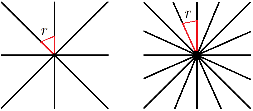
Refer to caption
Figure 5: For a given r>0r>0, compare how far one has to move from the point of intersection so that each line is at least a distance of rr from the other lines.
Refer to caption
Figure 6: Γk,Δ\Gamma^{k,\Delta} is depicted in blue, ∂Blj​(zj)\partial B_{l_{j}}(z_{j}) in red, and Γk,Δ∩Bls​(zs)\Gamma^{k,\Delta}\cap B_{l_{s}}(z_{s}) in black. The tick marks on the blue curves separate the arcs Aik,ΔA_{i}^{k,\Delta} outside of the disks. Although not all end points are shared by multiple curves Γk\Gamma^{k} in general, it is this case in the illustration above.

We then have the following:

Proposition 16.3.

Let NN be normal with spectrum in Γ\Gamma satisfying (∗)(\ast) and AA self-adjoint. Then if A,NA,N are almost commuting, they are nearly commuting.

Proof.

Let δ=‖[A,N]‖\delta=\|[A,N]\|. We apply the argument earlier to obtain HH finite range with respect to NN of distance Δ∼δγ0\Delta\sim\delta^{\gamma_{0}} such that ‖A−H‖≤C​o​n​s​t.δ1−γ0,‖[H,N]‖≤C​o​n​s​t.δ\|A-H\|\leq Const.\delta^{1-\gamma_{0}},\|[H,N]\|\leq Const.\delta. Recall (∗)(\ast).

Let ℬik,Δ\mathcal{B}^{k,\Delta}_{i}, 𝒱i,jk,Δ\mathcal{V}^{k,\Delta}_{i,j} be the range of the spectral projection of NN onto Aik,ΔA^{k,\Delta}_{i}, Ai,jk,ΔA^{k,\Delta}_{i,j}, respectively. We then obtain 𝒲ik,Δ\mathcal{W}^{k,\Delta}_{i} which are subspaces of the ℬik,Δ\mathcal{B}^{k,\Delta}_{i} that are almost invariant under Pℬik,Δ​H​Pℬik,ΔP_{\mathcal{B}^{k,\Delta}_{i}}HP_{\mathcal{B}^{k,\Delta}_{i}} such that 𝒱i,1k,Δ,s⊂𝒲ik,Δ⟂𝒱i,rik,Δ,sk,Δ,s\mathcal{V}^{k,\Delta,s}_{i,1}\subset\mathcal{W}^{k,\Delta}_{i}\perp{\mathcal{V}}^{k,\Delta,s}_{i,r^{k,\Delta,s}_{i}}. Let 𝒲ik,Δ,⟂=ℬik,Δ⊖𝒲ik,Δ\mathcal{W}^{k,\Delta,\perp}_{i}=\mathcal{B}^{k,\Delta}_{i}\ominus\mathcal{W}^{k,\Delta}_{i}.

We now need to deal with the subspace ℬΔ,s\mathcal{B}^{\Delta,s} projected onto by EBls​(zs)​(N)E_{B_{l_{s}}(z_{s})}(N). The issue is that because zsz_{s} can be the endpoint of multiple curves Γk\Gamma^{k}, we have to use a slightly different approach to form almost invariant subspaces of ℬΔ,s\mathcal{B}^{\Delta,s} so that everything works out. This is the only part of the proof where one uses a “two dimensional” grouping of eigenvalues of NN (using “polar coordinates”).

Fix an endpoint zsz_{s}. Let S1=Bℓs/2​(zs)S_{1}=B_{\ell_{s}/2}(z_{s}), Sik=Γk∩B(i−1)​Δ+ℓs/2​(zs)∖B(i−2)​Δ+ℓs/2​(zs)S_{i}^{k}=\Gamma^{k}\cap B_{(i-1)\Delta+\ell_{s}/2}(z_{s})\setminus B_{(i-2)\Delta+\ell_{s}/2}(z_{s}), SrΔ,sk=Γk∩Bls​(zs)∖B(rΔ,s−1)​Δ+ℓs/2​(zs)S_{r^{\Delta,s}}^{k}=\Gamma^{k}\cap B_{l_{s}}(z_{s})\setminus B_{(r^{\Delta,s}-1)\Delta+\ell_{s}/2}(z_{s}), where ℓs/2−1<rΔ,s​Δ≤ℓs/2\ell_{s}/2-1<r^{\Delta,s}\Delta\leq\ell_{s}/2. What we do is break ℬΔ,s\mathcal{B}^{\Delta,s} into orthogonal subspaces 𝒱1Δ,s,𝒱2k,Δ,s,…,𝒱rΔ,sk​Δ,s\mathcal{V}^{\Delta,s}_{1},\mathcal{V}^{k,\Delta,s}_{2},\dots,\mathcal{V}^{k\Delta,s}_{r^{\Delta,s}} by letting ES1​(N)E_{S_{1}}(N) project onto 𝒱1Δ,s\mathcal{V}^{\Delta,s}_{1} and ESik​(N)E_{S_{i}^{k}}(N) project onto 𝒱ik,Δ,s\mathcal{V}^{k,\Delta,s}_{i} for 1<i≤rΔ,s1<i\leq r^{\Delta,s}. Consider HΔ,s=PℬΔ,s​H​PℬΔ,sH^{\Delta,s}=P_{\mathcal{B}^{\Delta,s}}HP_{\mathcal{B}^{\Delta,s}} as a block matrix with respect to the subspaces 𝒱1Δ,s,𝒱2k,Δ,s,…,𝒱rΔ,sk​Δ,s\mathcal{V}^{\Delta,s}_{1},\mathcal{V}^{k,\Delta,s}_{2},\dots,\mathcal{V}^{k\Delta,s}_{r^{\Delta,s}}.

For each kk, we restrict HH to ℬk,Δ,s=𝒱1Δ,s⊕⨁i=2rΔ,s𝒱ik,Δ,s\mathcal{B}^{k,\Delta,s}=\mathcal{V}^{\Delta,s}_{1}\oplus\bigoplus_{i=2}^{r^{\Delta,s}}\mathcal{V}^{k,\Delta,s}_{i} to obtain Hk,Δ,sH^{k,\Delta,s}. Hk,Δ,sH^{k,\Delta,s} is tridiagonal with respect to the subspaces 𝒱1Δ,s,𝒱2k,Δ,s,…,𝒱rΔ,sk​Δ,s\mathcal{V}^{\Delta,s}_{1},\mathcal{V}^{k,\Delta,s}_{2},\dots,\mathcal{V}^{k\Delta,s}_{r^{\Delta,s}} which correspond to a set covering Γk∪S1\Gamma^{k}\cup S_{1} in Bℓs​(zs)B_{\ell_{s}}(z_{s}). Then there is a subspace 𝒲kΔ,s⊂ℬk,Δ,s\mathcal{W}^{\Delta,s}_{k}\subset\mathcal{B}^{k,\Delta,s} that is almost invariant under Hk,Δ,sH^{k,\Delta,s} such that 𝒱rΔ,sk,Δ,s⊂𝒲kΔ,s⟂𝒱1Δ,s\mathcal{V}^{k,\Delta,s}_{r^{\Delta,s}}\subset\mathcal{W}^{\Delta,s}_{k}\perp\mathcal{V}^{\Delta,s}_{1}.

Refer to caption
Figure 7: The point zsz_{s} is an endpoint for Γ1,Γ2,Γ3,\Gamma^{1},\Gamma^{2},\Gamma^{3}, and Γ4\Gamma^{4}. The small tick marks are the intersections of circles centered at zsz_{s} of radii i​Δi\Delta. The almost invariant subspaces 𝒲kΔ,s\mathcal{W}^{\Delta,s}_{k} are illustrated in red and 𝒲Δ,s⟂\mathcal{W}^{\perp}_{\Delta,s} in blue. Although these subspaces do not necessarily lie entirely within the span of the illustrated eigenspaces of NN, 𝒲Δ,s⟂\mathcal{W}^{\perp}_{\Delta,s} contains all eigenspaces of NN within distance ls/2l_{s}/2 of zsz_{s} and 𝒲kΔ,s\mathcal{W}^{\Delta,s}_{k} contains the eigenspaces depicted by part of the (red) spectrum near the large tick marks.

Now, P𝒲kΔ,s≤EΓ~k,Δ,s​(N)P_{\mathcal{W}^{\Delta,s}_{k}}\leq E_{\tilde{\Gamma}^{k,\Delta,s}}(N) so not only are the subspaces 𝒲kΔ,s\mathcal{W}^{\Delta,s}_{k} orthogonal for different values of kk, but HΔ,sH^{\Delta,s} maps 𝒲kΔ,s\mathcal{W}^{\Delta,s}_{k} into 𝒲kΔ,s⊕𝒱1Δ,s\mathcal{W}^{\Delta,s}_{k}\oplus\mathcal{V}^{\Delta,s}_{1} due to the assumption on the distance between the Γ~k,Δ,s\tilde{\Gamma}^{k,\Delta,s} for different values of kk. Hence, HΔ,sH^{\Delta,s} is equal to Hk,Δ,sH^{k,\Delta,s} on 𝒲kΔ,s\mathcal{W}^{\Delta,s}_{k} and HΔ,s​(𝒲kΔ,s)H^{\Delta,s}(\mathcal{W}^{\Delta,s}_{k}) is perpendicular to 𝒲k′Δ,s\mathcal{W}^{\Delta,s}_{k^{\prime}} for k′≠kk^{\prime}\neq k since 𝒲k′Δ,s⟂𝒱1Δ,s\mathcal{W}^{\Delta,s}_{k^{\prime}}\perp\mathcal{V}^{\Delta,s}_{1} by construction. Then we find that 𝒲kΔ,s\mathcal{W}^{\Delta,s}_{k} are almost invariant under HΔ,sH^{\Delta,s} because

(1−P𝒲kΔ,s)​HΔ,s​P𝒲kΔ,s=Pℬk,Δ,s⊖𝒲kΔ,s​Hk,Δ,s​P𝒲kΔ,s\displaystyle(1-P_{\mathcal{W}^{\Delta,s}_{k}})H^{\Delta,s}P_{\mathcal{W}^{\Delta,s}_{k}}=P_{\mathcal{B}^{k,\Delta,s}\ominus\mathcal{W}^{\Delta,s}_{k}}H^{k,\Delta,s}P_{\mathcal{W}^{\Delta,s}_{k}}

has small norm.

Let 𝒲Δ,s⟂=ℬΔ,s⊖⨁k𝒲kΔ,s\mathcal{W}^{\perp}_{\Delta,s}=\mathcal{B}^{\Delta,s}\ominus\bigoplus_{k}\mathcal{W}^{\Delta,s}_{k}. Because Hs,ΔH^{s,\Delta} is Hermitian, we have broken ℬΔ,s\mathcal{B}^{\Delta,s} into almost invariant subspaces 𝒲kΔ,s,𝒲Δ,s⟂\mathcal{W}^{\Delta,s}_{k},\mathcal{W}^{\perp}_{\Delta,s}.

We now form the new basis of subspaces ℬ~\tilde{\mathcal{B}}. This is a simple process, but its explanation is complicated by the fact that because of parity issues, we cannot just say “join 𝒲\mathcal{W}’s with 𝒲⟂\mathcal{W}^{\perp}’s” as before. We let the subspaces ℬ~\tilde{\mathcal{B}} include three types of subspaces. The first subspaces that we include are 𝒲Δ,s⟂\mathcal{W}^{\perp}_{\Delta,s}. The other “𝒲\mathcal{W}” subspaces contain a “𝒱{\mathcal{V}}” subspace which has to be matched with its neighboring “𝒱{\mathcal{V}}” subspace. One of the subspaces 𝒲ik,Δ,𝒲ik,Δ,⟂\mathcal{W}^{k,\Delta}_{i},\mathcal{W}^{k,\Delta,\perp}_{i} contains that subspace 𝒱isk,jskk,Δ\mathcal{V}^{k,\Delta}_{i_{s}^{k},j_{s}^{k}}, call this subspace 𝒲isk,jsk\mathcal{W}_{i_{s}^{k},j_{s}^{k}}. We then include the subspace 𝒲isk,jsk⊕𝒲kΔ,s\mathcal{W}_{i_{s}^{k},j_{s}^{k}}\oplus\mathcal{W}^{\Delta,s}_{k}. We also include the direct sums of the remaining consecutive subspaces 𝒲ik,Δ,⟂⊕𝒲i+1k,Δ\mathcal{W}^{k,\Delta,\perp}_{i}\oplus\mathcal{W}^{k,\Delta}_{i+1}.

Having defined the subspaces ℬ~\tilde{\mathcal{B}}, we proceed to defining the nearby commuting matrices. We define N′N^{\prime} to be the normal matrix that is block identity picking an eigenvalue from the arcs (or union of arcs) that we used to make the spaces ℬ~\tilde{\mathcal{B}}. We then have that N′N^{\prime} and H′=∑ℬ~Pℬ~​H​Pℬ~H^{\prime}=\sum_{\tilde{\mathcal{B}}}P_{\tilde{\mathcal{B}}}HP_{\tilde{\mathcal{B}}} commute and these matrices are within a distance of a power of Δ\Delta from NN and HH, respectively. ∎

ACKNOWLEDGEMENTS. The author would like to thank Eric A. Carlen for introducing the issue of [29] to the author and for helpful discussions about it, Matthew Hastings for some corrections of and clarifications concerning [29], and Ilya Kachkovskiy for providing feedback concerning the characterization of the constructiveness of [34] in the first version of this paper.

This research was partially supported by NSF grants DMS-2055282 and DMS-1764254.

References

  • [1] A.B. Aleksandrova, V.V. Peller. Estimates of operator moduli of continuity. Journal of Functional Analysis 261 (2011) 2741–2796.
  • [2] A. B. Aleksandrov and V. V. Peller. Operator Hölder-Zygmund Functions. arXiv:0907.3049
  • [3] A. B. Aleksandrov and V. Peller. Operator Lipschitz functions. 2016 Russ. Math. Surv.71 605.
  • [4] J. Bastian and K. Harrison. Subnormal Weighted Shifts and Asymptotic Properties of Normal Operators Proc. Amer. Math. Soc. 42 (1974), 475-479. https://doi.org/10.1090/S0002-9939-1974-0380491-X
  • [5] M. Benzi and G. Golub. Bounds for the Entries of Matrix Functions with Applications to Preconditioning. BIT Numerical Mathematics (1999) 39: 417. https://doi.org/10.1023/A:1022362401426
  • [6] I. Berg and C. Olsen. A note on Almost Commuting Matrices. Proc. R. Ir. Acad. Vol. 81A(1), 43-47 (1981)
  • [7] I. Berg. On Approximation of Normal Operators by Weighted Shifts. Michigan Math. J. 21(4): 377-383 (July 1975).
  • [8] R. Bhatia, C. Davis, and A. McIntosh. Perturbation of Spectral Subspaces and Solution of Linear Operator Equations. Linear Algebra and its Applications. 52/53:45-67 (1983) https://doi.org/10.1016/0024-3795(83)80007-X
  • [9] R. Bhatia, C.Davis and P. Koosis. An extremal problem in Fourier analysis with applications to operator theory. Journal of Functional Analysis 82, 138-150 (1989)
    https://doi.org/10.1016/0022-1236(89)90095-5
  • [10] R. Bhatia and P. Rosethal. How and Why to Solve the Operator Equation A​X−X​B=Y.AX-XB=Y. Bull. London Math. Soc. 29 (1997) 1-21 https://doi.org/10.1112/S0024609396001828
  • [11] B. Blackadar. Operator Algebras - Theory of C∗C^{\ast}-Algebras and von Neumann Algebras. Springer-Verlag. Berlin Heidelberg. 2006.
  • [12] O. Bratteli and D. Robinson. Operator Algebras and Quantum Statistical Mechanics. Volume 1. 1979.
  • [13] M.-D. Choi. Almost Commuting Matrices Need not be Nearly Commuting. Proceedings of American Mathematical Society. Vol 102. No 3. March 1988.
  • [14] K. Davidson. Almost Commuting Hermitian Matrices. Math. Scand. 56 (1985), 222-240.
  • [15] K. Davidson. C∗C^{\ast}-Algebras by Example. AMS. 1996.
  • [16] K. Davidson and S. Szarek “Local Operator Theory, random matrices and Banach spaces” Handbook of the Geometry of Banach Spaces. Vol I. Elsevier Science. 2001.
  • [17] C. Davis. Generators of the Ring of Bounded Operators. Proc. Amer. Math. Soc. Vol. 6, No. 6 (Dec., 1955), pp.970-972.
  • [18] C. Davis. The Rotation of Eigenvectors by a Perturbation. Journal of Mathematical Analysis and Applications 6, 159-173 (1963) https://doi.org/10.1016/0022-247X(63)90001-5
  • [19] C. Davis and W. Kahan. The Rotation of Eigenvectors by a Perturbation. III. SIAM J. Numer. Anal., 7(1), 1–46. 1970. https://doi.org/10.1137/0707001
  • [20] S. Demko, W. Moss, and P. Smith. Decay Rates for Inverses of Band Matrices. Mathematics of Computation, 43(168), 491-499. (1984) doi:10.2307/2008290
  • [21] J. Dixmier. Position relative de deux variétés linéaires fermées dans un espace de Hilbert.
  • [22] D. Enders and T. Shulman. Almost Commuting Matrices, Cohomology, and Dimension. arXiv:1902.10451
  • [23] P. Friis and M. Rørdam. Almost commuting self-adjoint matrices - a short proof of Huaxin Lin’s theorem. J. reine angew. Math 479 (1996). 121-131.
  • [24] L. Glebsky. Almost commuting matrices with respect to normalized Hilbert-Schmidt norm. arXiv:1002.3082
  • [25] L. Grafakos. Classical Fourier Analysis. 2nd Edition. 2008.
  • [26] P. Halmos. Two Subspaces. Trans. Amer. Math. Soc. 144 (1969), 381–389.
  • [27] P. Halmos. Some unsolved problems of unknown depth about operators on Hilbert space. Proceedings of the Royal Society of Edinburgh, 76A, 67-76, 1976. https://doi.org/10.1017/S0308210500019491
  • [28] M. Hastings. Making Almost Commuting Matrices Commute. Commun. Math. Phys. 291, 321–345 (2009)
  • [29] M. Hastings. Making Almost Commuting Matrices Commute. Version 4. arXiv:0808.2474
  • [30] M. Hastings. Personal Communication.
  • [31] M. Hastings and T. Loring. Almost commuting matrices, localized Wannier functions, and the quantum Hall effect. J. Math. Phys. 51, 015214 (2010). https://doi.org/10.1063/1.3274817
  • [32] D. Herrera. Constructing Nearby Commuting Matrices for Reducible Representations of s​u​(2)su(2) with an Application to Ogata’s Theorem. Preprint (to appear on arXiv.org).
  • [33] C. Jordan. Essai sur la géoméacutrie à nn dimensions.
  • [34] I. Kachkovskiy and Y. Safarov. Distance to Normal Elements in C∗C^{\ast}-Algebras of Real Rank Zero. Journal of the American Mathematical Society, 2016-01, Vol.29 (1), p.61-80
  • [35] H. Lin. Almost commuting self-adjoint matrices and applications. Fields. Inst. Commun. 13, 193 (1995).
  • [36] T. Loring and A. Sørensen. Almost-Commuting Self-Adjoint Matrices - The Real and Self-Dual Cases. Reviews in Mathematical Physics, 28(07): 1650017, 2016.
  • [37] W. Luxemburg and R. Taylor. Almost Commuting Matrices are near Commuting Matrices. Indagationes Mathematicae (Proceedings). Volume 73, 1970, pp 96-98
  • [38] D. Nagaj, P. Wocjan, Y. Zhang. Fast Amplification of QMA. https://arxiv.org/abs/0904.1549
  • [39] Y. Ogata. Approximating macroscopic observables in quantum spin systems with commuting matrices. Journal of Functional Analysis. Vol. 264, Issue 9, 1 May 2013, pp 2005-2033.
  • [40] T. Osborne. Almost Commuting Unitaries with Spectral Gap are Near Nearly Commuting Matrices. Proc. Amer. Math. Soc. Vol 137, No 12, December 2009, pp4043-4048
  • [41] C. Pearcy and A. Shields. Almost Commuting Matrices. Journal of Functional Analysis. 33, 332-338 (1979).
  • [42] S. Pironio. et al. Device-independent quantum key distribution secure against collective attacks. 2009 New J. Phys.11 045021
  • [43] A. Prakash. Quantum Algorithms for Linear Algebra and Machine Learning. Dissertation. https://www2.eecs.berkeley.edu/Pubs/TechRpts/2014/EECS-2014-211.html
  • [44] P. Rosenthal. Are Almost Commuting Matrices Near Commuting Matrices? The American Mathematical Monthly, Vol. 76, No. 8 (Oct., 1969), pp. 925-926.
  • [45] M. Said. Almost Commuting Elements in Non-Commutative Symmetric Operator Spaces. Dissertation.
  • [46] E. Stein and R. Shakarchi. Complex Analysis. Princeton University Press. 2003.
  • [47] S. Szarek. On Almost Commuting Hermitian Operators. Rocky Mountain Journal of Mathematics. Vol. 20, No. 2, Spring 1990.
  • [48] D. Voiculescu. Asymptotically commuting finite rank unitary operators without commuting approximants. Acta Sci. Math. (Szeged) 45:1-4(1983), 429-431 1983.