Unraveling the origin of magnetic fields in galaxies2020Unraveling the origin of magnetic fields in galaxies–13
Abstract
Despite their ubiquity, there are many open questions regarding galactic and cosmic magnetic fields. Specifically, current observational constraints cannot rule out if magnetic fields observed in galaxies were generated in the Early Universe or are of astrophysical nature. Motivated by this we use our magnetic tracers algorithm to investigate whether the signatures of primordial magnetic fields persist in galaxies throughout cosmic time. We simulate a Milky Way-like galaxy down to in four scenarios: magnetised solely by primordial magnetic fields, magnetised exclusively by SN-injected magnetic fields, and two combined primordial + SN magnetisation cases. We find that once primordial magnetic fields with a comoving strength G are considered, they remain the primary source of galaxy magnetisation. Our magnetic tracers show that, even combined with galactic sources of magnetisation, when primordial magnetic fields are strong, they source the large-scale fields in the warm metal-poor phase of the simulated galaxy. In this case, the circumgalactic and intergalactic medium can be used to probe without risk of pollution by magnetic fields originated in the galaxy. Furthermore, whether magnetic fields are primordial or astrophysically-sourced can be inferred by studying local gas metallicity. As a result, we predict that future state-of-the-art observational facilities of magnetic fields in galaxies will have the potential to unravel astrophysical and primordial magnetic components of our Universe.
Keywords:
MHD - methods: numerical - galaxies: formation - galaxies: magnetic fields - galaxies: spiral1 Introduction
From planets and stars to clusters of galaxies, magnetic fields pervade our Universe on all scales. Their importance is well recognised in most astrophysical scenarios, be it the process of star formation (Vázquez-Semadeni et al. 2011; Federrath & Klessen 2012; Krumholz & Federrath 2019), the propagation of cosmic rays (Kulsrud & Pearce 1969), or the their role in active galactic nuclei (AGN) residing in galaxy clusters (Weinberger et al. 2017; Bambic et al. 2018; Ehlert et al. 2018).
For galaxies in particular, magnetic fields are generally observed at low redshift to have energies comparable or even above the thermal and turbulent energies of the gas (Beck 2007; Beck 2015, e.g.), corresponding to field strengths of order (Chyzy et al. 2011; Basu & Roy 2013; Mulcahy et al. 2014). Magnetic fields may play an important role in processes shaping galaxies such as star formation (Padoan & Nordlund 2011; Zamora-Avilés et al. 2018), the evolution of galactic outflows (Grønnow et al. 2018), the mixing of gas in galaxy haloes (van de Voort et al. 2020), and regulation of the structure and dynamics of the multi-phase interstellar medium (Iffrig & Hennebelle 2017; Körtgen et al. 2019, ISM;). When their energy is comparable to the kinetic and thermal energies of the gas, magnetic fields can affect the global properties of galaxies (Pillepich et al. 2018; Martin-Alvarez et al. 2020) or even reduce the galaxy stellar mass function (Marinacci & Vogelsberger 2016). As a result, magnetic fields are an important contributor to the process of galaxy formation.
Notwithstanding their importance, the origin of magnetic fields in galaxies and at large scales remains unknown. Amongst the various possibilities to generate these magnetic fields, three primary channels persist (Rees 1987). Two of them are astrophysical in nature: dynamical amplification mechanisms (Dubois & Teyssier 2010; Beck et al. 2012; Pakmor & Springel 2013, e.g.), or feedback through magnetised outflows from point-like sources such as stars or AGN (Beck et al. 2013). Alternatively, magnetic fields could have a primordial origin, with strong fields generated in the early Universe and then preserved and evolved with the baryonic gas (Ratra 1992; Barrow & Tsagas 2011, e.g.). Cosmological simulations have shown the viability of astrophysical mechanisms to produce magnetic fields through turbulent dynamo amplification (Dolag et al. 1999; Pakmor et al. 2014; Rieder & Teyssier 2017b; Martin-Alvarez et al. 2018; Vazza et al. 2018) of weak seed fields generated by e.g., a Biermann battery (Attia et al. 2021). Similarly, the injection of magnetic fields by supernova (SN) events can also produce the magnetic fields observed in galaxies (Butsky et al. 2017; Katz et al. 2019). Equivalently, AGN could play a similar role for galaxy clusters (Vazza et al. 2017), whereas their role in galaxies is yet to be explored in detail. Finally, if the magnetic fields generated in the early evolution of our Universe are strong enough, they will be amplified to strengths in galaxies during the collapse of density perturbations (Kandus et al. 2011) even though additional dynamo amplification might be required for galaxy clusters (Vazza et al. 2017). A variety of theoretical models advocate the production of strong magnetic fields during the early Universe, e.g. during the process of inflation (Ratra 1992; Sharma et al. 2018). For comprehensive reviews on the origin of magnetic fields in our Universe see Widrow 2002; Kandus et al. 2011; Subramanian 2016.
Determining the primordial magnetic field of the Universe is an arduous task. In the absence of direct measurements of intergalactic magnetic fields (Taylor et al. 2015) permeating cosmic scales, the most reliable prospect is placing upper and lower limits on their strength. However, current constraints allow an exceedingly large range of values that do not adequately constrain the importance of primordial magnetic fields. A well-accepted upper limit for the primordial magnetic field strength11 1 When discussing the strength of primordial magnetic field or cosmological magnetic fields, their strength can be determined at different scales. Unless indicated otherwise, we will refer generally to magnetic fields with coherence lengths Mpc. Furthermore, the strength of will be provided in comoving units. is G, provided by the absence of B-mode signal induced by primordial magnetic fields in the perturbations of the cosmic microwave background (Planck Collaboration 2015, CMB;). More stringent upper constraints can be extracted from other probes such as the propagation of ultra-high energy cosmic rays (UHECRs) through the intergalactic medium (IGM). Measuring the offset in their arrival direction from their predicted sources, Bray & Scaife 2018 claim an upper limit G. Obtaining a lower limit for is even more problematic, as potential signatures of magnetic fields at large scales rapidly weaken as their strength decreases. Nonetheless, Neronov & Vovk 2010 proposed a lower limit G based on the non-detection of secondary GeV emission when observing TeV blazars. This has been contested (Broderick et al. 2012, e.g. by), as plasma instabilities could dissipate the energy of particle pairs prior to the GeV emission. More recently, Broderick et al. 2018 also found a non-detection of inverse Compton GeV emission in oblique lines-of-sight to TeV sources. This non-detection places an upper limit inconsistent with (i.e. with a lower value than) the lower limits by Neronov & Vovk 2010. Other canonical lower limits tend to be much weaker (e.g. G based on the Harrison mechanism; Hutschenreuter et al. 2018), and thus do not elucidate the uncertainty surrounding primordial magnetic fields. This illustrates the need for further study before limits on primordial magnetic fields are well-understood. As a result, it is important to consider alternatives that could aid our understanding of the cosmic magnetic field.
In the advent of facilities such as SKA, which may directly detect magnetic fields in filaments (Govoni et al. 2019) or those permeating the IGM (Gaensler et al. 2004; Beck 2014), cosmological simulations are the perfect tool to guide and interpret these observations (Vazza et al. 2017, e.g.). However, when studying the origin of magnetic fields, one of the issues is that various channels of magnetisation will operate simultaneously. As a result, simulations must study their co-evolution and devise a method to disentangle magnetic fields of different origins. This can be done using the magnetic tracing method proposed in Katz et al. 2019. In that paper, we presented the first application of such an algorithm, based on linearly decomposing the total magnetic field in the simulation into multiple extra magnetic fields. A useful decomposition is to then associate each additional tracer magnetic field with a particular origin or magnetic energy source. In this method the total magnetic field (i.e. the only field allowed to influence the dynamics) and the tracer fields are evolved in time solving the induction equation for each of them separately. As a result, the code allows us to unravel for the first time the exact contribution made by each source of magnetism to the magnetisation of a simulation. In this work we apply this method to investigate the co-evolution of primordial and astrophysical magnetic fields in a cosmological zoom-in simulation of a galaxy, disentangling the effects and properties of each type of magnetic field. As upcoming surveys will provide the community with a vast range of observations of magnetic fields in galaxies, we revise whether galaxies and their surroundings can be used to probe and measure the cosmic magnetic field of our Universe.
This work is organized as follows: the numerical methodology to generate and evolve our simulations is described in Section 2 as well as the tracer algorithm (Section 2.5). Section 3 explores our main results, subdivided according to the various properties we consider. Due to the numerical approximations and physical models employed in this work, in Section 4 we discuss the implications of our findings and the most important caveats. Finally, we conclude with a summary of our work in Section 5.
2 Numerical methods
2.1 The RAMSES code
The magnetohydrodynamical (MHD) zoom-in simulations of galaxy formation explored in this work are produced using our own modified version of the public code ramses (Teyssier 2002). ramses employs an adaptive mesh refinement (AMR) octree grid to solve the evolution of the baryonic gas. This gas is coupled through gravity to the dark matter and stars which we model as collisionless particles. The evolution of the magnetic field in ramses is calculated using a constrained transport (CT) method. It models magnetic fields as face-centred quantities, ensuring that the divergence constraint () is exactly conserved numerically (Teyssier et al. 2006; Fromang et al. 2006). We employ our magnetic field tracer algorithm (Katz et al. 2019, presented in), which is an extension of the CT solver in ramses, to follow the evolution of magnetic fields attending to their origin. Section 2.5 provides more details on the configuration used for the magnetic tracers. The magnetic diffusivity in most astrophysical environments is considerably below the numerical diffusivity of ramses at the spatial resolutions considered in this study. As a result, we set in the induction equation used to evolve the magnetic field
| (1) |
Consequently, all diffusive effects in our simulations are of numerical nature.
2.2 Initial conditions
The setup of our simulation follows the evolution of a Milky Way (MW) like galaxy in the high resolution region of a cosmological zoom-in run (nut; Powell et al. 2011). The cubic box has a side of 12.5 comoving Mpc (cMpc), containing a zoom sphere of cMpc across. Stellar and dark matter particles in this zoom region have mass resolutions of and , respectively. We allow refinement to resolve the octree grid down to a minimum physical cell size of pc in this region. A grid cell above this minimum size is refined into 8 equal cells when it contains within itself at least 8 dark matter particles or when its total mass (i.e. accounting for baryonic and dark matter) is above , where and are the mass density and baryonic mass density parameters, respectively. The studied galaxy is the most massive system forming in the high resolution region, with a halo virial mass . Cosmological parameters are selected according to the WMAP5 cosmology (Dunkley et al. 2009).
2.3 Further physics
To realistically model galaxy formation, we include in all our simulations the following subgrid physics prescriptions. The process of reionization is modelled by a UV background switched on at (Haardt & Madau 1996). We account for gas metal cooling above and below K interpolating cloudy cooling tables (Ferland et al. 1998) and according Rosen & Bregman 1995 respectively. We always assume the baryonic gas to be ideal and mono-atomic, with specific heat ratio .
To simulate the formation of stars, we use a magneto-thermo-turbulent star formation model, presented in its thermo-turbulent form by Kimm et al. 2017; Trebitsch et al. 2017 adopting an extension to account for magnetic fields as in Martin-Alvarez et al. 2020. In order to form stars, a gas cell must fulfill the following two constraints:
- •
it must exist on the highest level of refinement (Rasera & Teyssier 2006) at the current redshift, and
- •
the gravitational pull on the gas must be higher than the local combination of turbulent, magnetic, and thermal support.
In those cells where star formation is allowed, the star formation rate follows a simple Schmidt law (Schmidt 1959)
| (2) |
with being the gas density and the free-fall time. The star formation efficiency is a local value that depends on the magneto-thermodynamical properties of the host and neighbouring gas cells. The efficiency follows the Padoan & Nordlund 2011 model as described by Federrath & Klessen 2012. For more details see Appendix B of Martin-Alvarez et al. 2020.
We model SN events using the mechanical stellar feedback prescription of Kimm & Cen 2014; Kimm et al. 2015 in which a star particle injects mass, momentum and energy back to its host cell and its neighbours. We assume a Kroupa initial mass function (Kroupa 2001), where each SN event injects a specific energy of . Each explosion returns a fraction of the total exploding mass to the ISM gas , of which is returned as metals.
2.4 Two origins for the galactic magnetic field


In this work, we investigate the properties and evolution of two fundamentally different types of magnetic fields in galaxies: magnetic fields with a primordial origin versus magnetic fields of galactic/astrophysical nature. The first will be generated prior to the onset of our simulations, whereas the second will be sourced throughout the galaxy formation process. Due to the absence of source terms in the induction equation (Equation 1), we can model the two sources of interest by two distinct procedures. We will model primordial magnetic fields as an ab-initio magnetic field. More specifically, our simulations will have a uniform and homogeneous magnetic field (divergenceless by construction) oriented along the z-axis of the simulated box, with a constant comoving strength . The second source of magnetic fields will be modelled by magnetising SN ejecta. We insert small-scale closed loops of magnetic field around each SN event adjusted to produce a magnetic energy . This value is comparable with those used by other authors: e.g. by Beck et al. 2013, by Butsky et al. 2017, by Vazza et al. 2017. The vast majority of our SN events take place at the highest level of refinement, which implies that the typical size of each injected loop is 10 physical pc. We find our choice to typically inject realistic magnetic fields of G (Parizot et al. 2006, e.g.) when injected over these 10 pc scales. We provide more details on the magnetic injection method in Appendix A.
Due to limitations in spatial resolution, the temporal rate of turbulent amplification in galaxy formation simulations such as those studied here is low compared with that expected in the real ISM. While similar simulations with magnetic fields in the kinematic regime are able to produce relatively fast amplification (e.g. departing from G seeds; Rieder & Teyssier 2016; Martin-Alvarez et al. 2018), this is not the case for the magnetic fields studied in this work. Here our galaxies rapidly reach fields across their volume with strengths shortly after their formation (), either through primordial or SN-injection seeding. Therefore, we expect minor turbulent dynamo activity, which will in turn only produce a limited growth of the magnetic energy (Rieder & Teyssier 2017a). Consequently, the two sources of magnetic field described above are the main drivers of the galactic magnetic energy, whereas the turbulent dynamo would only be considered an important contender when contributing to the final magnetic energy budget if the magnetic field in the galaxy was weaker. Note that other dynamical processes such as e.g. disk shear (after disk formation at ) will also influence the evolution of the two traced magnetic fields. We discuss this in Section 4. Our selection of is motivated by observations and previous work. is selected instead with the specific aim of directly obtaining realistic magnetisations in the simulated galaxy. We show in Section 3.1 that our choices for the and yield both primordial and SN-injected magnetic fields of comparable strength in all runs, pointing towards saturated magnetisations. Similarly, the typical magnetic fields in the simulated galaxy compare well with those deduced by observations. Therefore, the ab-initio magnetic field G will be a good representation of a primordial magnetic field that provides realistic magnetisation for similar ramses cosmological simulations of spiral galaxies. In contrast, the SN-injected magnetic field will depict a star-sourced magnetic field, but will also serve as a rough approximation for other galactic channels of magnetisation: e.g. a small-scale turbulent dynamo produced magnetic field.
| Simulation | Stellar feedback | (G) | Tracers | Further details | ||
|---|---|---|---|---|---|---|
| B12prim | 10 pc | Mechanical | ✗ | ✗ | Reference for primordial magnetic field-only scenario | |
| B20SN | 10 pc | Mechanical | ✗ | Reference for astrophysical sources-only scenario | ||
| B12primSN | 10 pc | Mechanical | ✓ | Astrophysical vs. primordial (primordial dominated) | ||
| B13primSN | 10 pc | Mechanical | ✓ | Astrophysical vs. primordial (astro. dominated) |
While there is uncertainty about whether primordial magnetic fields are prominent in our Universe, we expect astrophysical magnetisation to be relevant in most scenarios. As a result, we require an understanding of the effects of each of these sourcing mechanisms separately, as well as of their combined role. Through four different simulations, we compare all these scenarios for the two sources of magnetisation. Each simulation is named BX where determines the strength of G. If the primordial magnetic field modelled is dynamically important, the simulation has the suffix prim added to its name. Similarly, if SN-injection is included, the name contains the suffix SN. Simulations with both a G (i.e. prim) and SN injection include our magnetic tracers. The four simulated galaxies are shown in Figure 1 and correspond to:
- •
B12prim: a purely primordial magnetisation scenario with a strong primordial magnetic field ( G, ). The magnetisation of the galaxy is dominated by the choice of .
- •
B20SN: an exclusively astrophysical origin for magnetic fields ( G, ). This run represents the case in which the primordial magnetic field is extremely weak and galaxy magnetisation takes place in-situ.
- •
B12primSN: a combination of a prominent primordial magnetic field and astrophysical sourcing ( G, ). This run combines the two different magnetisation scenarios with our tracing algorithm to explore the co-evolution of the two fields with a strong primordial magnetisation.
- •
B13primSN: as a final addition to our suite, we include a simulation similar to B12primSN but with a slightly weaker primordial magnetic field ( G, ). This simulation will allow us to place a lower bound for the importance of primordial magnetic fields in the magnetisation of the studied galaxy.
Due to the computational cost, we evolve all the runs to and only continue B12primSN to . The divergenceless behaviour of all runs is shown in Fig. 2. It depicts the ratio of divergence to magnetic field, which informs on the relative importance of numerical errors, but not on their absolute values. The average of the ratio between the local magnetic divergence and magnetic fields remain significantly below the percent level, with maximum values corresponding to O- and X-points. We note that our injection mechanism produces O-points by construction and yields higher divergences, but even their maxima remain smaller than the magnetic field at all times. All simulations are summarised in Table 1.
2.5 Disentangling the magnetic field sources
All our simulations use the MHD equations to follow directly the evolution of the total magnetic field . On top of this, we employ the method we presented in Katz et al. 2019 to decompose the total magnetic field into two separate fields. These two additional fields are sourced by either (primordial) or (astrophysical). As a result, they always add up to the total magnetic field . Each of these fields is evolved independently through the induction equation and equally fulfils the solenoidal constraint. Neither of the two tracer fields interacts with the gas dynamics and can in this way be understood as a colour field.
The first magnetic colour will correspond to the primordial magnetic field, and is simply set by requiring at the beginning of the simulation. The second magnetic colour will be the astrophysical magnetic field, set to initially and injected (sourced) by magnetised feedback as the simulation progresses. Whenever a SN event takes place with , both and are modified (as described in Appendix A). This separation into magnetic colours is illustrated in the right column of Fig. 1, where the colour green represents the magnetic energy associated with and the red colour corresponds to the magnetic energy found for .
When separating the magnetic field into two magnetic tracers, the total magnetic energy density can be decomposed into three terms
| (3) |
where the last term on the right hand side is the product of the interaction between the two magnetic fields. We will refer to this term as the cross-term magnetic energy. We note that the misalignment of and will allow this term to become negative. This term is shown in the rightmost column of Fig. 1 as the blue colour. We discuss the meaning of the other colours in the rightmost column in Section 3.2. Throughout the paper, we will associate the green colour with a primordial magnetic field, the red colour with SN-injected magnetic fields, and the blue colour with the energy resulting from the interaction of the two tracer fields.
3 Results
3.1 Realistic magnetic fields in the galaxy: different origins, similar energy
In Fig. 3 we show the specific magnetic energy in the galactic region. We define the galactic region as a sphere centred on the galaxy with radius , where is the virial radius of the dark matter halo. The centre of the region is determined by applying our version of the halomaker software (Tweed et al. 2009) to the baryonic mass, and recursively computing the central position through the shrinking spheres method (Power et al. 2003). Fig. 3 shows that the galaxy has the same approximate magnetisation in all four simulations. B12prim has the lowest due to our particular choice of , whereas B20SN has a slightly higher specific magnetic energy, due to a more efficient injection in the absence of pre-existing magnetic fields (see Appendix A). Nonetheless, the attained level of magnetisation does not allow us to distinguish between the origin of the magnetic field across these simulations. The global properties of galaxies are predicted to undergo only minor changes due to magnetic fields, unless greater magnetisations are explored (Su et al. 2017; Pakmor et al. 2017; Marinacci et al. 2015; Martin-Alvarez et al. 2020). For value of used by B12prim, Martin-Alvarez et al. 2020 showed that the impact of magnetic fields on the properties of the galaxy is modest. As B12primSN, B13primSN, and B20SN all have similar magnetisations to B12prim, we expect the general properties of all our galaxies to be similar. This is apparent in the mock observations and gas projections in Fig. 1. We also validate our galaxies against observations using the stellar mass-halo mass relation and their typical magnetic fields (see Fig. 4 and associated discussion).
Fig. 1 shows projections for the galaxy in each of the studied runs. The left column shows a composite colour mock observation in rest-frame SDSS [, , ] filters. We model the obscuration by dust purely as absorption, approximating the dust mass in a given cell as of the metal mass (Kaviraj et al. 2016). The central column presents a gas density-weighted projection for the gas density (cyan), gas temperature (red), and magnetic energy density (green). These two panels depict a gas-rich galaxy with an extended star forming disk at approximately the beginning of Cosmic Noon - the peak of star formation of the Universe at . The appearance of the galaxy in the mock observations and gas density projections is considerably similar across runs, indicating that the different initial and injected magnetic fields portrayed do not cause significant differences between the systems. This is expected, as we have shown that all four galaxies have comparable magnetic energy budgets (Fig. 3).
In Fig. 4, we compare the simulated galaxy with two observational relations. In the top panel, we show the stellar mass vs halo mass relation. All runs have approximately the same median halo and stellar masses at . They are found in relatively good agreement with the relations by Behroozi et al. 2013 and Moster et al. 2018 at and , where the shaded bands show dispersion. To avoid an excess of stellar mass, simulations typically calibrate the intensity of stellar feedback (Crain et al. 2015; Rosdahl et al. 2018, e.g.). This aims to replace typically unaccounted for physics such as magnetic fields, cosmic rays, and radiation. While our galaxies have an excess of stellar mass compared to the empirical relations (factor of ), we opt not to do a calibration of the SN feedback in order to explore the topic at hand using the standard physical values attributed to and (see further discussion in Section 4). The bottom panel shows the average magnetic field vs star formation rate (SFR). The SFR is measured as the mass of stars in the galaxy with an age lower than Myr in a given snapshot - the mass of young stars, divided by a Myr time interval. Data points and error bars correspond to the time-weighted median and upper and lower quartiles of all snapshots in the interval , combining typically snapshots per simulation. The average magnetic field in our galaxy is in good agreement with the order of magnitude found in observations ().
3.2 Unraveling the origin of magnetic fields
The right-most column of Fig. 1 displays the three forms of traced magnetic energy density: SN-injected (red), primordial (green), and cross-term (blue). In these projections, whenever the cross-term is negative, it is removed in equal parts from and . Due to the colour composition employed, yellow tones correspond to regions featuring high values of both and . Conversely, cyan and violet tones are respectively a mixture of and , or and . While a number of interesting properties can be appreciated in the two runs with tracers, perhaps the most striking feature is that and cannot be clearly differentiated in any region of the galaxy. All of the galaxy is instead a combination of the three different magnetic energies, both for the case of B12primSN (primordial dominated) and B13primSN (SN-injection dominated). However, Fig. 1 indicates that there is a radial transition to one of the two tracers dominating as the distance from the centre increases. The outskirts of B12primSN are primordially dominated whereas the SN-injected energy dominates in the outer regions of B13primSN. The primordially-dominated run also appears to have a more radially extended magnetisation than the SN-injected case. This could be expected, as these primordial magnetic fields should be ubiquitous at all scales (Vazza et al. 2017 find a similar result at larger scales). We will review in more detail the radial distribution of the different types of magnetic energy in Section 3.3. These projections showcase an important conclusion recurrent through this work: primordial magnetic fields with strengths G are non-negligible in the magnetisation and evolution of galaxies. They dominate the magnetic energy budget in these systems at least up to , past the peak of star formation of the Universe, and potentially until the present day. G was also found in Martin-Alvarez et al. 2020 to be the approximate magnetic field above which noticeable effects on the global properties of galaxies due to the presence of magnetic fields manifest, with larger effects when studying even stronger .
To review more quantitatively how magnetic energy sources compare in B12primSN and B13primSN, we show in Fig. 5 their corresponding specific magnetic energies, separated into magnetic energy tracers. The upper panels show these for the galactic region (), while the bottom panels show the same quantities for the remainder of the halo (). Both runs have a total (solid lines) specific magnetic energy (and magnetic energy density ) in the galactic region. Fig. 5 confirms that when decomposed into magnetic tracers (dashed lines), B12primSN is dominated by the primordial magnetic field (green dashed lines) whereas B13primSN is dominated by the SN-injected magnetic field (red dashed lines). The discussion of the cross-term energy (dashed blue line for the positive/constructive fraction and dashed purple line for the negative/destructive fraction) is deferred until the end of this Section. While for B12primSN, the two tracer energies contain a significant fraction of the total magnetic energy (at , both energies are comparable ), is secondary for B13primSN.
To facilitate the analysis of the relative importance of each tracer field, we show the ratio of each traced magnetic energy to the total magnetic energy in Fig. 6. Primordial, SN-injected, positive cross-term and negative cross-term are once again shown by green, red, blue, and purple coloured lines, respectively. Each row shows a radial slice of the dark matter halo. Left and right columns show these measurements for B12primSN and B13primSN, respectively.
Similar ratios for each traced magnetic energy are observed in the halos: B12primSN is primordially dominated (after , ), whereas the magnetic energy in the halo of B13primSN is dominated by the outflows from the galaxy. Understanding the magnitude of astrophysically-generated magnetic fields expelled to the CGM (circumgalactic medium), the distances they reach into the IGM, as well as their volume fraction and relative importance with respect to primordial magnetic fields is paramount for observations desiring to constrain the cosmic magnetic field using measurements around galaxies as a proxy (Neronov & Vovk 2010; Broderick et al. 2018, e.g.). If primordial magnetic fields are strong (e.g., G), it will be unlikely that observations are polluted by astrophysical magnetic fields. In B12primSN, drops below at kpc, with kpc. In contrast, the primordial magnetic energy in B13primSN only becomes outside the halo ( kpc). Note that the indicated distances are only lower limits, as additional physics, such as cosmic rays, could potentially enhance the driving of galactic winds (Salem et al. 2014; Dashyan & Dubois 2020) and even increase their magnetisation (Ruszkowski et al. 2017). Furthermore, we do not account for AGN in our simulations, but these are expected to be active at some point during the evolution of typical MW-like galaxies (Heywood et al. 2019a). Similarly, AGN-driven winds may be considerable even in dwarf galaxies (Koudmani et al. 2019; Koudmani et al. 2020, see e.g.), with AGN capable of polluting the primordial magnetic field around galaxies with a range of masses. We discuss this issue further in Section 4, and defer the inclusion of AGN to future work. If the studied is high, the importance of primordial magnetic fields in the halo at high redshift continually increases in time as additional pristine and magnetised gas is accreted by the system. After , all slices of the B12primSN halo remain dominated by primordial magnetic energy. Furthermore, we find that in the halo of a galaxy indicates the existence of strong primordial magnetic fields (according to the caveats discussed in Section 4).
In the presence of a disk, galactic outflows will preferentially emerge perpendicularly to its plane. Thus, it is interesting to review the distribution of the different types of magnetic energy across the sky. All-sky Mollweide projections of the simulated galaxies at are shown in Fig. 7. For each projection, we place an observer at the galactic centre and divide the sky using a HEALPix decomposition (Gorski et al. 2005). Each pixel projects cells with an angular distance from the pixel centre , with angular resolution . The map is shown in Mollweide coordinates, where the equatorial poles are aligned with the galactic angular momentum. Fig. 7 is an RGB colour composite for the SN-injected (red) and primordial (green) magnetic energies - blue colour is omitted for clarity. In agreement with our previous results, primordial magnetic fields dominate B12primSN at all radii. The top left map shows the galactic region (the inner pc are ignored to avoid projection effects), where the galactic disk is evidenced by the amber band along the equator. The colour indicates that in the disk, both SN-injected and primordial magnetic fields are comparable. The top left and the top middle () maps have SN-injected magnetic energy prevailing at latitudes above and below the equator. However, in the top right (), bottom left (), and bottom right () panels the distribution is more homogeneous and randomised. While primordial magnetic fields are more important, certain smaller regions exist that are dominated by SN-injected magnetic fields. Due to this, and the complex morphology of the magnetic field, some degree of primordial magnetic field pollution is expected in haloes, unless G. These more extreme primordial magnetic fields have been shown to have other potential signatures of their presence including modified properties of galaxies or reionisation histories (Marinacci & Vogelsberger 2016; Safarzadeh & Loeb 2019; Martin-Alvarez et al. 2020; Sanati et al. 2020; Katz et al. 2021, e.g.). B13primSN is globally dominated by the SN tracer magnetic field, and portrays a more patchy magnetisation at the outskirts of the halo. There are some filaments that are magnetised by the primordial component. Interestingly, as we move from the inner to the outer region of the halo, the coherence length of magnetic energy structures appears to increase, most likely correlated with the coherence of bulk velocity flows, as well as the initialisation of the primordial magnetic field as a uniform field (Marinacci et al. 2015). We will explore in Sections 3.5 and 3.6 whether the origin of the magnetic fields in the halo can be distinguished by examining gas properties such as temperature or metallicity.


Up until this point, we have not discussed the cross-term magnetic energy resulting from the interaction between the two types of magnetic fields considered. Figs. 5 and 6 show that the cross-term magnetic energy is typically well below the other two types of energies. The proportionality of the cross-term with both tracers in Equation 3 suppresses the importance of this cross energy when one of the tracers comprises the majority of the magnetic field. As a result, the cross-term energy is unimportant in the halos () of B12primSN and B13primSN, and equally so for the B13primSN galaxy. In contrast, the galactic region of B12primSN features both significant and , which leads to a non-negligible contribution of the cross-term. Our maximisation of the injected energy per loop (described in Appendix A) leads to the injection mechanism predominantly injecting positive cross-term energy. Interestingly, the negative cross-term is above the positive fraction in the galactic region of B12primSN throughout most of the simulation (Fig. 6). We attribute this to the behaviour of the magnetic tracers during magnetic reconnection. If two reconnecting magnetic lines are associated with different tracers, the total magnetic field cancels. However the traced magnetic fields superimpose in anti-alignment, producing a negative contribution to the cross-term. The turbulent nature of the ISM causes significant magnetic reconnection, which in turn increases the negative cross-term. In contrast, in the simulated halo of B12primSN, the positive cross-term energy is prevalent due to bulk motions mostly driven by galactic outflows and the low amount of turbulence. Nonetheless, the cross-term energy is seldom comparable to the SN-injected energy and mostly unimportant with respect to the primordial budget. The high fraction of cross-term magnetic energy in B12primSN indicates a substantial interaction between the two traced magnetic fields, thus both being important for the magnetic effects taking place in the galaxy.
We have shown in this Section that primordial magnetic fields are prevalent in galaxies and their haloes when their comoving strength is G. We now proceed to examine how the energy is distributed spatially across the galaxy.
3.3 The spatial separation of astrophysical and primordial magnetic fields
Due to their intrinsic properties, each channel of magnetisation is more important in different regions of the galaxy. Magnetic fields produced by stars will concentrate in the extended gas disk and the centre of the galaxy, where most star formation occurs. Conversely, primordial magnetic fields are initially amplified by compressional processes when pristine gas is accreted onto the cosmic web, and eventually fed to the outskirts of galaxies. As a result, the relative importance of primordial magnetisation will be higher at large radii. To quantitatively explore the spatial distribution of the magnetic field in the galaxy, we show in Fig. 8 the total and traced magnetic fields mass-weighted radial profiles22 2 We find that employing a volume-weighted measurement yields unchanged results, but reduces the typical values of by dex. at . The profiles are computed using cylindrical coordinates for thin cylinders of and half-thickness pc, where the z-coordinate is aligned with the angular momentum of the galactic baryonic mass. The left and right columns show the profiles for the B12primSN and B13primSN runs, respectively. Different rows correspond from top to bottom to the total magnetic field () and the axial to total (), radial to total (), and toroidal to total () magnetic field ratios. Each panel presents the combined (i.e. the sum of both tracers) magnetic field (thick solid line), and its decomposition into SN-injected (red dashed) and primordial (green dashed) magnetic fields. For further comparison, we include the profiles for the B12prim (thin green solid line) and B20SN (thin red solid line) simulations, which only consider one source of magnetic field. Finally, we include the profiles calculated by Berkhuijsen et al. 2016 for M101, Beck 2015 for IC342, and Basu & Roy 2013 for NGC5236 and NGC6949, which portray galaxies with size and morphology comparable to our system.
We focus on first, for which we find various interesting features. All profiles display a break at about kpc, corresponding to the approximate gas disk radial extension. Within kpc, all profiles are relatively flat, with . However, SN-injected magnetic fields (B20SN and the corresponding tracer in B12primSN and B13primSN) progressively increase in their strength towards the centre of the galaxy. On the contrary, magnetic fields of primordial nature (B12prim and the primordial magnetic field tracer in B12primSN and B13primSN) have a shallower horizontal profile with a more constant at all radii. As a result, even though the magnetic field in the majority of the B12primSN disk is dominated by the primordial component, the inner kpc of the disk is dominated by an astrophysical magnetic field. In fact, we expect astrophysical magnetic fields to dominate in the centre of most galaxies, even more so in the presence of AGN. In B12primSN, the difference in the slopes of each magnetic tracer profile leads to the dominance of primordial magnetic fields at kpc. Finally, for weaker primordial magnetic fields (i.e. B13primSN) is always dominated by fields generated in the galaxy. Our profiles are in good agreement with the observations shown in Fig. 8. We note that the observed galaxies are found at , whereas our system is studied at higher redshift. This comparison assumes that the behaviour we find between and is conserved down to . While there is evidence supporting the existence of comparable magnetic fields in galaxies at redshifts as high as (Bernet et al. 2008), their radial distribution might have some redshift evolution. Similarly, M101 extends to larger radii than our system (Berkhuijsen et al. 2016, report a break of the profile at approximately 16 kpc). At the centre of the observed galaxies, the profiles portray weaker magnetic fields than our simulations. However, this is likely due to a lack of resolution. For example, Aitken et al. 1998 estimate magnetic fields as high as mG at the centre of the MW. These strong magnetic fields would be in better agreement with the astrophysically-amplified magnetic fields in our simulations. The profiles have a similar behaviour to those obtained by Pakmor et al. 2017.
We decompose the magnetic field into a cylindrical component, finding a similar behaviour across the four simulations. is approximately constant at all radii. In contrast, slightly decreases at small and large radii. increases at large distances due to bulk flow accretion onto the disk. When reviewing the behaviour of the two tracer fields we find that their interrelation is, as expected, mostly dictated by the modulus of each tracer field (i.e. top panels). However, we note that the aforementioned increase of at larger distances has a larger reflection on the primordial magnetic field tracer field.
The apparent equipartition of the magnetic tracers across the three coordinates is likely caused by the turbulent, small-scale magnetic field, for which we expect all coordinates to be equidistributed. Dominance of the strength of the magnetic field by its turbulent component is also found in observations (Beck 2015, e.g.). We have shown that primordial magnetic fields with G dominate at intermediate radii of galactic disks and become even more important at the outskirts. As a result, it is now interesting to pin down at which scales each tracer dominates. One possibility would be to examine whether this behaviour is still in place when separating turbulent and large-scale magnetic fields (Ntormousi et al. 2020, e.g. as done by). We leave this for future work and opt instead to explore the magnetic energy spectra, which provides a better overview of the relevant scales for magnetic fields. This will help us answer whether strong primordial magnetic fields could be responsible for the large scale magnetic fields that we observe in galaxies (Nixon et al. 2018).
3.4 The prevalence of primordial magnetic field at large scales in galaxies
Due to their vectorial nature, magnetic fields distribute their energy differently across the span of spatial scales. To unfold this information, it is useful to study the magnetic energy spectra in Fourier space. We compute our spectra through the Fast Fourier Transform33 3 We acknowledge the use of the FFTW library (http://www.fftw.org/). (FFT) of 1024 cells-per-side cubic boxes centred at the position of the galaxy, onto which the entire AMR structure is interpolated. We fix the box size to 26 kpc, assuming periodic boundary conditions in our FFT computation44 4 Appendix B in Martin-Alvarez et al. 2018 discusses how periodicity affects these type of spectra in FFT transformations.. To reach higher resolutions, we decide not to 0-pad our FFT, but we note that this would yield a more pronounced decay of power towards the lower values. Finally, to aid comparison between the different runs, we normalise the spectra to the value of the total magnetic field in the main run of each panel. These runs are B12primSN (amber solid line) and B13primSN (orange solid line) for the left and right panels of Fig. 9. Green and red solid lines show the spectra for the B12prim and B20SN runs. Finally, the dashed lines in each panel are the spectra resulting from the FFT applied to each magnetic tracer in the corresponding run.
The energy spectra of the magnetic tracers reveal striking differences according to the source of the magnetisation. Magnetic fields of primordial nature have more power at scales larger than the galaxy () due to the environmental magnetisation and higher field at large radii. For the SN-injected field, we observe a more pronounced decay towards smaller due to the magnetic field being produced within the galaxy. At intermediate scales, spanning from the size of the galaxy to the thickness of the disk (), we find a relatively flat spectrum for primordial fields, accumulating power at . This suggests that primordial magnetic fields dominate and peak at the large-scales of B12primSN. In contrast, the SN-injected fields have a more pronounced inverse-cascade that continues to grow up to the smallest scales of the intermediate range (). SN-injected fields peak at a scale of approximately pc, roughly the thickness of the disk and slightly above the scale at which SN forcing is most efficient. We expect the magnetisation of hot gas in large SN bubbles to be fully governed by this magnetisation channel. This is shown and further discussed in Section 3.5. Finally, at the smallest scales (), both fields decay due to the limited resolution and the convolution with the disk of the galaxy (see Appendix B, Martin-Alvarez et al. 2018). However, we find a steeper decline of the primordial magnetic energy spectrum towards larger than of the SN-injected one. This is in agreement with an injection scale of approximately the size of the disk for the primordial fields whereas the SN-injected ones are generated at the smallest scales in our simulation. Finally, when focusing on our primary simulation, B12primSN, we find an interesting change of regime at the scale of the disk, : the large-scale magnetic fields of the galaxy are dominated by a primordial origin whereas the small-scale field has an astrophysical one. Our spectra suggest that magnetic fields produced by SN are not as efficiently re-organised into large-scale magnetic fields as those of primordial origin. As a result, if the magnetic field of the Universe is G, we predict galactic-scale magnetic fields to be the remnants of magnetic fields originated in the early Universe. We discuss other considerations that might be important for this statement in Section 4. Finally, the overall behaviour observed for the tracers is also confirmed by our simulations with only one magnetisation channel. That is: B20SN resembles the SN-injected tracer, whereas B12prim is similar to the primordial magnetic field-tracer.
3.5 The distribution of magnetic fields across ISM phases


In the same manner our two traced magnetic fields have distinct scales of injection into the galaxy, the thermodynamical properties of the magnetised gas are different for each channel. Pristine gas is mostly accreted through cold flows whereas SN-injected magnetic fields are produced in hot SN bubbles. We explore the distribution of the traced magnetic energies across the temperature - density phase space in Fig. 10. Plot colours showcase the ratio between two types of tracer energies, which are determined by the colour scale. We include contours depicting the absolute energy distribution. The first column in Fig. 10 corresponds to the galactic region in B13primSN (top) and B12primSN (bottom). They are coloured according the ratio of SN-injected (red colour) to primordial (green colour) magnetic energy (). Contours show the distribution of the total magnetic energy (white, ). For comparison, we also include the total magnetic energy contours for B20SN (orange) and B12prim (green). The distribution of total magnetic energy is comparable across runs, with a more substantial concentration in the warm phase ( K, ) when primordial magnetic fields are present, and higher magnetic energy in the hot gas ( K) when injection is included. For the weaker case (B13primSN), the magnetic energy is dominated by the SN-injected energy across the entire phase space. B12primSN is more intriguing: in the cold and dense phase of the galaxy ( K, ) SN-injected magnetic fields prevail. However, at intermediate densities () primordial magnetic fields dominate. Altogether with Section 3.4, this suggests that the large-scale magnetic fields permeating the warm phase of the galaxy are the remnants of primordial magnetism for G. As expected, the hottest gas is produced in SN events, and therefore magnetised by the astrophysical magnetic energy tracer. The behaviour portrayed by these two panels is in place from approximately onward.
The central column shows the two same plots, now coloured by the ratio of SN-injected to absolute cross-term energy (). Contours show the distribution of the positive (blue lines) and negative (purple lines) parts of the cross term energy. The cross-term energy is generally unimportant, except in the cold and dense phase. Here, both galaxies feature a non-negligible contribution from the negative cross-term energy. This supports that magnetic reconnection is large in the galaxy, with the majority of the interaction between the two tracers taking place in the phase space boundary between the warm-cold phases. However, we note that the cross-term energy does not fully dominate the energy budget in any region of the phase space.
Finally, we want to understand how magnetic fields are distributed in the halo of the galaxy, in particular for G, as future observations may probe the CGM and IGM to determine the magnetic field of our Universe. In the right-most column of Fig. 10 we show the ratio of SN-injected to primordial (top; ) and primordial to absolute cross (bottom; ) magnetic energies for the outer region of the halo () in the B12primSN simulation. Once again white contours show the distribution of the total magnetic energy. While the energy budgets discussed in Section 3.2 show that SN-generated magnetic fields are secondary in the halo of the galaxy, Fig. 10 indicates that SN-generated magnetic fields are still present at the highest temperatures.
3.6 The magnetic field - metallicity correlation


If magnetic fields are generated by stars, or primarily inside galaxies, we expect a correlation of the magnetic field associated with a parcel of gas and its metallicity. This correlation has been shown to hold in isolated galaxies (Butsky et al. 2017) and in their halo (Pakmor et al. 2019). These two studies find that this correlation holds for magnetisation of astrophysical (inside the galaxy) nature, either by SN-injection or dynamical amplification, respectively. In this Section we review whether this correlation also holds for primordial magnetic fields, and taking advantage of our tracer algorithm, we also show whether strong primordial magnetic fields can be identified and discerned from astrophysical ones by means of studying the local gas metallicity.
In Fig. 11 we colour the phase space as a function of the ratio between two traced magnetic energies at for the B12primSN (top row) and B13primSN (bottom row) simulations. As before, white contours show the distribution of the total magnetic energy and whenever present, cyan and orange show the total magnetic energy in the B12prim (exclusively primordial) and B20SN (exclusively astrophysical) runs, respectively. The first two columns show the ratio of SN-injected to primordial magnetic energy in the galactic region (left column) and the external part of the halo (right column; ). Both in the galaxies and their haloes we find a clear separation of SN and primordial magnetic fields, with the former concentrating at higher metallicities and the second at pristine gas. When comparing the distribution of the total magnetic energies, the one generated inside the galaxy accumulates more uniformly across metallicities , whereas the primordial energy has a flatter distribution towards the lowest metallicities in the simulation. The low metallicity but high magnetic field region of the phase diagram is particularly interesting, as SN-produced magnetic fields do not seem capable to penetrate it. Attending to our tracer simulations, we predict the presence of strong magnetic fields ( G) in regions of extremely low metal content to be a signature of primordial magnetic fields. These could be measured in the CGM of galaxies even when accounting for the pollution of galactic magnetic fields. Additional physics or the calibration of our employed feedback prescription might drive more efficient galactic outflows that may introduce some pollution of this low metallicity / high magnetic field regime dominated by primordial magnetic fields. When reviewing the correlation of the magnetic field with metallicity in the galactic region. We fit assuming magnetic energy-weighting. Low correlations are found for simulations dominated by primordial magnetic fields B12prim () and B12primSN (). However, when the runs are dominated by SN injection the values found for are higher: for B20SN and for B13primSN55 5 Mass-weighted values for B12prim, B12primSN, B20SN, and B13primSN are respectively .. These two regimes of correlation are also found when separating the magnetic energy in B12primSN into the two tracer fields, with and . This indicates that even in the presence of various magnetic sources, the division based on metallicity is maintained. In the rightmost column of Fig. 11 we show the ratio of primordial to cross-term magnetic energy in the halo of both galaxies (B12primSN, top; B13primSN, bottom). Altogether with the central column, this confirms that any potential pollution by astrophysically-generated magnetic fields in the low-metallicity region is unimportant both for SN-injected magnetic fields and for the energy produced by the interaction between the two magnetic fields.
4 Discussion and caveats
We have shown that strong primordial magnetic fields (i.e. G) produce realistic galactic magnetisation, compatible with observations and comparable with the one attained when magnetic fields are instead the product of SN feedback. Furthermore, we have found that when primordial and SN-generated magnetic fields are considered in combination, the attained magnetisation is not distinguishable from any of the two former cases. In a similar study, Garaldi et al. 2020 found a comparable result when evolving a zoom simulation of a galaxy to , exploring separately magnetisation from either a Biermann battery (Biermann 1950), the Durrive & Langer 2015 mechanism, a primordial seed, or SN injection. They find their SN and primordial channels provide a galaxy magnetisation roughly indistinguishable by . We note that they probe a weaker primordial seed ( G) and a lower magnetic energy injection by SN () than those studied here. As a result, their considered channels of galaxy magnetisation rely more significantly on dynamical amplification than those in our work. We also find that the origin of galactic magnetic fields cannot be discriminated based on magnetisation once they have reached comparable levels, shortly after the formation of the studied galaxy in our work. However, we have found using our magnetic field tracing algorithm that in our simulations strong primordial magnetic fields and those produced inside the galaxy have differentiated properties and can be distinguished from high redshift () onwards. In particular, we find changes in their energy distribution across spatial scales, as well as in terms of correlations with ISM temperature and gas metallicity. This differentiation can be taken advantage of by future observations, using galaxies as probes of the cosmic magnetic field and potentially improving our constraint of its upper limit ( G; Planck Collaboration 2015) by up to three orders of magnitude.
However, a series of important considerations must be taken into account when interpreting the results presented in this work. Firstly, we only considered two main channels of magnetic field generation, namely primordial (in the form of an ab-initio uniform field) and SN-injected magnetic fields. A third suitable channel of magnetic field generation in galaxies is through the action of a small-scale turbulent dynamo, which would amplify weak magnetic fields to values on short timescales. In the scenarios considered here, one can interpret the SN-injected magnetic fields as a proxy for magnetic fields amplified by a turbulent dynamo, as both are generated at the smallest scales in the simulated galaxy. We remark that no important turbulent dynamo activity is expected in our simulations: due to limited resolution, our CT method has modest magnetic amplification growth rates. This is even true when the magnetic field is weak and only in the kinematic regime (Martin-Alvarez et al. 2018). Furthermore, as the magnetic fields in our simulations rapidly reach , we expect their back-reaction on small-scales to inhibit the activity of the turbulent dynamo. As a result, small-scale dynamo amplification would only play a secondary role in our study, and would be more relevant for the SN-injected component of the field that prevails at small scales (Section 3.4). Our separation into two tracer fields can safely be interpreted as separating magnetic fields produced either inside the galaxy or in the early Universe. Apart from the turbulent dynamo, other dynamo processes are expected to be active in our galaxy. These will correspondingly modify dynamically the evolution of the total and traced magnetic fields through the induction equation (Equation 1). An example is shear and differential rotation of the galactic disk after its formation at (Chamandy et al. 2013; Bendre et al. 2015).
Secondly, as shown by Fig. 4, our galaxies have an excess of stellar mass for their given halo mass compared with expected relations (Behroozi et al. 2013; Moster et al. 2018, e.g.). A frequent solution employed by simulations to avoid this is to increase feedback efficiency by e.g., increasing the specific energy of stellar feedback, which thwarts the process of star formation. The excess of stellar mass in our simulations implies that more SN-events than expected for a Milky-Way mass galaxy are likely to occur. This in turn could overestimate the amount of SN-injected magnetic energy. As the main conclusion presented in this work is that strong primordial magnetic fields ( G) remain important in the studied galaxy down to , well after the peak of star formation of the Universe, the presence of additional SN-injected energy only reinforces this conclusion.
As our simulations are only evolved until ( for the B12primSN case), our comparison with observations at (e.g. as those presented in Fig. 8) relies on the assumption that no significant redshift evolution takes places between and . Evidence for strong magnetic fields has been observed at redshifts as high as (Bernet et al. 2008), but other field properties may differ. Similarly, the behaviour observed in our simulations remains approximately unchanged between and . However, as our simulations do not reach , some of their properties, including their deviation from the stellar mass vs halo mass may evolve if they were to reach this redshift.
When studying magnetic fields in the halo of galaxies, we find no significant evidence for dynamo activity in these regions. While halo dynamo amplification is often deemed unimportant (Beck et al. 2012; Marinacci et al. 2015; Butsky et al. 2017), Pakmor et al. 2019 suggested that some degree of amplification might occur once simulations reach high enough spatial resolution. If halo dynamo activity in nature causes an important amplification of weak primordial magnetic fields to values G, this would complicate a clear detection of primordial magnetic fields in the CGM of galaxies.
While the primordial magnetic field seeded in this work is uniform and homogeneous for the sake of simplicity, the primordial magnetic field of our Universe will be inhomogeneous and likely to approximately follow a power spectrum (Planck Collaboration 2015; Hutschenreuter et al. 2018). One of the potential consequences is that employing a uniform seed instead of an spectrum could imprint large-scale features on the simulated primordial field, particularly outside of virialised structures (Marinacci et al. 2015). Therefore, it is important to consider that, regardless of whether primordial magnetic fields are strong or weak in nature, different regions of the Universe will present local variations of the strength and importance of the primordial magnetic field.
Finally, we note that current galaxy formation simulations often lack additional physics that are important to capture the correct properties of the ISM. While we account for magnetic fields, radiative transfer (Rosdahl et al. 2015; Emerick et al. 2018) and cosmic rays (Pfrommer et al. 2017; Hopkins et al. 2019; Dashyan & Dubois 2020) influence the ISM of galaxies and the evolution of their magnetic fields (Hanasz et al. 2009). Equally, while AGN activity could be relatively unimportant in the explored mass regime (Crain et al. 2015; Martín-Navarro & Mezcua 2018), this mode of feedback could serve as a considerable source of magnetic fields as well as also producing magnetised outflows (Dashyan et al. 2018; Koudmani et al. 2019) such as those observed in the MW (Heywood et al. 2019b). Indeed, Vazza et al. 2017 show that AGN can eject magnetic fields to intergalactic distances. The importance of AGN in magnetising galaxies and their surroundings will be revisited with our magnetic tracers method in future work.
5 Conclusions
In this work we study four new magneto-hydrodynamical cosmological zoom-in simulations of a Milky Way-like galaxy. The simulations are generated using our modified version of the constrained transport MHD ramses code (Teyssier 2002; Fromang et al. 2006; Teyssier et al. 2006) capable of tracing the separate evolution of different types of magnetic fields (Katz et al. 2019). In particular, we trace magnetic fields of primordial nature as well as astrophysical magnetic fields generated in the galaxy during SN events. Our simulations span the cases of exclusively primordial (B12prim), primordially dominated (B12primSN), SN-injection dominated (B13primSN), and purely SN-injected (B20SN) magnetisation. With the focus on disentangling the primordially generated magnetic fields from the SN-injected ones in our simulations (B12primSN and B13primSN), we find the following results:
- 1.
Both primordial magnetic fields (with G) and SN-injected magnetic fields (with ) produce realistic magnetisations in simulated galaxies, and compare well with observations.
- 2.
Specifically, the profiles of the magnetic field in all our simulations compare well with observations (Basu & Roy 2013; Beck et al. 2005; Berkhuijsen et al. 2016, e.g.), and are similar to other MHD simulations (Pakmor et al. 2017). While the profile of primordial magnetic fields appear a better match to observations at the core of the galactic disk, this is likely due to the lack to resolution in observations as magnetic fields on the order of G are observed in the centre of our own galaxy (Aitken et al. 1998).
- 3.
The studied channels of magnetisation and their combinations produce galaxies with a similar appearance and almost identical stellar masses and star formation rates. This is in agreement with previous studies, which have suggested magnetic fields to have a minor impact on such properties (Pakmor et al. 2017; Su et al. 2017; Martin-Alvarez et al. 2020).
- 4.
Once strong enough primordial magnetic fields are considered with G, their resulting magnetic energy budget in galaxies is roughly equal to that attained by magnetic fields generated through SN feedback. G is the approximate value found in Martin-Alvarez et al. 2020 for which the first noticeable effects in galaxy properties due to magnetic fields appear. For even higher values of , primordial magnetic fields will have a significant impact on the global properties of galaxies.
- 5.
In the inner regions of the galaxy, bipolar outflows from the galaxy pollute the halo with SN-injected magnetic fields, which mostly concentrate at small radii ( kpc). The strong primordial fields are distributed approximately homogeneously and become dominant at larger distances ( kpc) as also evidenced by the analysis of magnetic energy spectra. This indicates that observations of magnetic fields in the CGM and IGM are potential probes of the primordial magnetic field of our Universe.
- 6.
Moreover, while SN-injected fields are dominant in hot SN-driven bubbles and outflows, strong primordial fields dominate in the warm phase of the ISM. While both type of fields correlate well with gas metallicity they scale in different way, with only the strong primordial fields found in pristine gas, which may help to unravel their origin.
Anticipating facilities that will be capable of unveiling the magnetic Universe, such as SKA, we showed that galaxies and their CGM are a potential window to the primordial magnetic field of our Universe. As emerging numerical work highlights the importance of magnetic fields, MHD simulations of galaxy formation will become an important tool to understand galaxy formation. In future work, we aim to study detailed mock observational signatures associated with our magnetic tracers which will allow us to make a direct link with observations to ultimately unravel the origin of cosmic magnetic fields.
Acknowledgements
We kindly thank the referee for insightful comments and suggestions that contributed to improve the quality of this manuscript. We would like to thank Jim Pringle and Franco Vazza for useful comments and suggestions. DS would like to thank Prof. D’Anchise for all the help and support in finalizing this manuscript. This work was supported by the ERC Starting Grant 638707 “Black holes and their host galaxies: co-evolution across cosmic time" and by STFC. This work is part of the Horizon-UK project, which used the DiRAC Complexity system, operated by the University of Leicester IT Services, which forms part of the STFC DiRAC HPC Facility (www.dirac.ac.uk). This equipment is funded by BIS National E-Infrastructure capital grant ST/K000373/1 and STFC DiRAC Operations grant ST/K0003259/1. The equipment was funded by BEIS capital funding via STFC capital grants ST/K000373/1 and ST/R002363/1 and STFC DiRAC Operations grant ST/R001014/1. DiRAC is part of the National e-Infrastructure. The authors would like to acknowledge the use of the University of Oxford Advanced Research Computing (ARC) facility in carrying out this work. http://dx.doi.org/10.5281/zenodo.22558. The authors also acknowledge the usage of the FFTW library: http://www.fftw.org/. Some of the results in this paper have been derived using the healpy and HEALPix package (http://healpix.sourceforge.net; Zonca et al. 2019).
Data availability
The data employed in this manuscript is to be shared upon reasonable request contacting the corresponding author.
References
- Aitken et al. (1998) Aitken D. K., Smith C. H., Moore T. J., Roche P. F., 1998, Monthly Notices of the Royal Astronomical Society, 299, 743
- Attia et al. (2021) Attia O., Teyssier R., Katz H., Kimm T., Martin-Alvarez S., Ocvirk P., Rosdahl J., 2021, MNRAS, 000, 1
- Bambic et al. (2018) Bambic C. J., Morsony B. J., Reynolds C. S., 2018, The Astrophysical Journal, 857, 84
- Barrow & Tsagas (2011) Barrow J. D., Tsagas C. G., 2011, Monthly Notices of the Royal Astronomical Society, 414, 512
- Basu & Roy (2013) Basu A., Roy S., 2013, Monthly Notices of the Royal Astronomical Society, 433, 1675
- Beck (2007) Beck R., 2007, Astronomy and Astrophysics, 470, 539
- Beck (2014) Beck R., 2014, Springer, Berlin, Heidelberg, pp 3–17, doi:10.1007/978-3-662-44625-6_1, http://link.springer.com/10.1007/978-3-662-44625-6_1
- Beck (2015) Beck R., 2015, Astronomy & Astrophysics, 578, A93
- Beck et al. (2005) Beck R., Fletcher A., Shukurov A., Snodin A., Sokoloff D. D., Ehle M., Moss D., Shoutenkov V., 2005, Astronomy & Astrophysics, 444, 739
- Beck et al. (2012) Beck A. M., Lesch H., Dolag K., Kotarba H., Geng A., Stasyszyn F. A., 2012, Monthly Notices of the Royal Astronomical Society, 422, 2152
- Beck et al. (2013) Beck A. M., Dolag K., Lesch H., Kronberg P. P., 2013, Monthly Notices of the Royal Astronomical Society, 435, 3575
- Behroozi et al. (2013) Behroozi P. S., Wechsler R. H., Conroy C., 2013, Astrophysical Journal, 770, 57
- Bendre et al. (2015) Bendre A., Gressel O., Elstner D., 2015, Astronomische Nachrichten, 336, 991
- Berkhuijsen et al. (2016) Berkhuijsen E. M., Urbanik M., Beck R., Han J. L., 2016, Astronomy and Astrophysics, 588, A114
- Bernet et al. (2008) Bernet M. L., Miniati F., Lilly S. J., Kronberg P. P., Dessauges-Zavadsky M., 2008, Nature, 454, 302
- Biermann (1950) Biermann L., 1950, Zeitschrift Naturforschung Teil A, 5, 65
- Bray & Scaife (2018) Bray J. D., Scaife A. M. M., 2018, The Astrophysical Journal, 861, 3
- Broderick et al. (2012) Broderick A. E., Chang P., Pfrommer C., 2012, The Astrophysical Journal, 752, 22
- Broderick et al. (2018) Broderick A. E., Tiede P., Chang P., Lamberts A., Pfrommer C., Puchwein E., Shalaby M., Werhahn M., 2018, The Astrophysical Journal, 868, 87
- Butsky et al. (2017) Butsky I., Zrake J., Kim J.-h., Yang H.-I., Abel T., 2017, The Astrophysical Journal, 843, 113
- Chamandy et al. (2013) Chamandy L., Subramanian K., Shukurov A., 2013, Monthly Notices of the Royal Astronomical Society, 428, 3569
- Chyzy et al. (2011) Chyzy K. T., Wezgowiec M., Beck R., Bomans D. J., 2011, Astronomy and Astrophysics, 529
- Crain et al. (2015) Crain R. A., et al., 2015, Monthly Notices of the Royal Astronomical Society, 450, 1937
- Dashyan & Dubois (2020) Dashyan G., Dubois Y., 2020, Astronomy and Astrophysics, 638, A123
- Dashyan et al. (2018) Dashyan G., Silk J., Mamon G. A., Dubois Y., Hartwig T., 2018, Monthly Notices of the Royal Astronomical Society, 473, 5698
- Dolag et al. (1999) Dolag K., Bartelmann M., Lesch H., 1999, Astronomy and Astrophysics, 348, 351
- Dubois & Teyssier (2010) Dubois Y., Teyssier R., 2010, Astronomy & Astrophysics, 523, A72
- Dunkley et al. (2009) Dunkley J., et al., 2009, Astrophysical Journal, Supplement Series, 180, 306
- Durrive & Langer (2015) Durrive J. B., Langer M., 2015, Monthly Notices of the Royal Astronomical Society, 453, 345
- Ehlert et al. (2018) Ehlert K., Weinberger R., Pfrommer C., Pakmor R., Springel V., 2018, Monthly Notices of the Royal Astronomical Society, 481, 2878
- Emerick et al. (2018) Emerick A., Bryan G. L., Mac Low M.-M., 2018, The Astrophysical Journal, 865, L22
- Federrath & Klessen (2012) Federrath C., Klessen R. S., 2012, Astrophysical Journal, 761, 156
- Ferland et al. (1998) Ferland G. J., Korista K. T., Verner D. A., Ferguson J. W., Kingdon J. B., Verner E. M., 1998, Publications of the Astronomical Society of the Pacific, 110, 761
- Fromang et al. (2006) Fromang S., Hennebelle P., Teyssier R., 2006, Astronomy & Astrophysics, 457, 371
- Gaensler et al. (2004) Gaensler B., Beck R., Feretti L., 2004, New Astronomy Reviews, 48, 1003
- Garaldi et al. (2020) Garaldi E., Pakmor R., Springel V., 2020, MNRAS, 000, 1
- Gorski et al. (2005) Gorski K. M., Hivon E., Banday A. J., Wandelt B. D., Hansen F. K., Reinecke M., Bartelmann M., 2005, The Astrophysical Journal, 622, 759
- Govoni et al. (2019) Govoni F., et al., 2019, Science, 364, 981
- Grønnow et al. (2018) Grønnow A., Tepper-García T., Bland-Hawthorn J., 2018, The Astrophysical Journal, 865, 64
- Haardt & Madau (1996) Haardt F., Madau P., 1996, The Astrophysical Journal, 461, 20
- Hanasz et al. (2009) Hanasz M., Wóltański D., Kowalik K., 2009, Astrophysical Journal, 706, L155
- Heywood et al. (2019a) Heywood I., et al., 2019a, Nature, 573, 235
- Heywood et al. (2019b) Heywood I., et al., 2019b, Nature, 573, 235
- Hopkins et al. (2019) Hopkins P. F., et al., 2019
- Hutschenreuter et al. (2018) Hutschenreuter S., Dorn S., Jasche J., Vazza F., Paoletti D., Lavaux G., Enßlin T. A., 2018, Classical and Quantum Gravity, 35, 154001
- Iffrig & Hennebelle (2017) Iffrig O., Hennebelle P., 2017, Astronomy & Astrophysics, 604, A70
- Kandus et al. (2011) Kandus A., Kunze K. E., Tsagas C. G., 2011, Primordial magnetogenesis, doi:10.1016/j.physrep.2011.03.001, https://www.sciencedirect.com/science/article/pii/S0370157311000536?via%3Dihub
- Katz et al. (2019) Katz H., Martin-Alvarez S., Devriendt J., Slyz A., Kimm T., 2019, Monthly Notices of the Royal Astronomical Society, 484, 2620
- Katz et al. (2021) Katz H., et al., 2021, MNRAS, 000, 1
- Kaviraj et al. (2016) Kaviraj S., et al., 2016, Monthly Notices of the Royal Astronomical Society, 467, stx126
- Kimm & Cen (2014) Kimm T., Cen R., 2014, Astrophysical Journal, 788, 121
- Kimm et al. (2015) Kimm T., Cen R., Devriendt J., Dubois Y., Slyz A., 2015, Monthly Notices of the Royal Astronomical Society, 451, 2900
- Kimm et al. (2017) Kimm T., Katz H., Haehnelt M., Rosdahl J., Devriendt J., Slyz A., 2017, Monthly Notices of the Royal Astronomical Society, 466, stx052
- Körtgen et al. (2019) Körtgen B., Banerjee R., Pudritz R. E., Schmidt W., 2019, Monthly Notices of the Royal Astronomical Society, 489, 5004
- Koudmani et al. (2019) Koudmani S., Sijacki D., Bourne M. A., Smith M. C., 2019, Monthly Notices of the Royal Astronomical Society, 484, 2047
- Koudmani et al. (2020) Koudmani S., Henden N. A., Sijacki D., 2020, MNRAS, 000, 1
- Kroupa (2001) Kroupa P., 2001, Monthly Notices of the Royal Astronomical Society, 322, 231
- Krumholz & Federrath (2019) Krumholz M. R., Federrath C., 2019, Technical report, The Role of Magnetic Fields in Setting the Star Formation Rate and the Initial Mass Function, https://arxiv.org/pdf/1902.02557.pdf. https://arxiv.org/pdf/1902.02557.pdf
- Kulsrud & Pearce (1969) Kulsrud R., Pearce W. P., 1969, The Astrophysical Journal, 156, 445
- Marinacci & Vogelsberger (2016) Marinacci F., Vogelsberger M., 2016, Monthly Notices of the Royal Astronomical Society: Letters, 456, L69
- Marinacci et al. (2015) Marinacci F., Vogelsberger M., Mocz P., Pakmor R., 2015, Monthly Notices of the Royal Astronomical Society, 453, 3999
- Martin-Alvarez et al. (2018) Martin-Alvarez S., Devriendt J., Slyz A., Teyssier R., 2018, Monthly Notices of the Royal Astronomical Society, 479, 3343
- Martin-Alvarez et al. (2020) Martin-Alvarez S., Slyz A., Devriendt J., Gómez-Guijarro C., 2020, Monthly Notices of the Royal Astronomical Society, 495, 4475
- Martín-Navarro & Mezcua (2018) Martín-Navarro I., Mezcua M., 2018, The Astrophysical Journal, 855, L20
- Moster et al. (2018) Moster B. P., Naab T., White S. D., 2018, Monthly Notices of the Royal Astronomical Society, 477, 1822
- Mulcahy et al. (2014) Mulcahy D. D., et al., 2014, Astronomy & Astrophysics, 568, A74
- Neronov & Vovk (2010) Neronov A., Vovk L., 2010, Science, 328, 73
- Nixon et al. (2018) Nixon C. J., Hands T. O., King A. R., Pringle J. E., 2018, Monthly Notices of the Royal Astronomical Society, 477, 3539
- Ntormousi et al. (2020) Ntormousi E., Tassis K., Del Sordo F., Fragkoudi F., Pakmor R., 2020
- Padoan & Nordlund (2011) Padoan P., Nordlund A., 2011, Astrophysical Journal, 730, 40
- Pakmor & Springel (2013) Pakmor R., Springel V., 2013, Monthly Notices of the Royal Astronomical Society, 432, 176
- Pakmor et al. (2014) Pakmor R., Marinacci F., Springel V., 2014, Astrophysical Journal Letters, 783, L20
- Pakmor et al. (2017) Pakmor R., et al., 2017, Monthly Notices of the Royal Astronomical Society, 469, 3185
- Pakmor et al. (2019) Pakmor R., et al., 2019
- Parizot et al. (2006) Parizot E., Marcowith A., Ballet J., Gallant Y. A., 2006, Astronomy and Astrophysics, 453, 387
- Pfrommer et al. (2017) Pfrommer C., Pakmor R., Schaal K., Simpson C. M., Springel V., 2017, Monthly Notices of the Royal Astronomical Society, 465, 4500
- Pillepich et al. (2018) Pillepich A., et al., 2018, Monthly Notices of the Royal Astronomical Society, 473, 4077
- Planck Collaboration (2015) Planck Collaboration 2015, Astronomy & Astrophysics, 594, A19
- Powell et al. (2011) Powell L. C., Slyz A., Devriendt J., 2011, Monthly Notices of the Royal Astronomical Society, 414, 3671
- Power et al. (2003) Power C., Navarro J. F., Jenkins A., Frenk C. S., White S. D. M., Springel V., Stadel J., Quinn T., 2003, Monthly Notices of the Royal Astronomical Society, 338, 14
- Rasera & Teyssier (2006) Rasera Y., Teyssier R., 2006, Astronomy & Astrophysics, 445, 1
- Ratra (1992) Ratra B., 1992, Technical report, Cosmological seed magnetic field from Inflation, http://articles.adsabs.harvard.edu/pdf/1992ApJ...391L...1R. http://articles.adsabs.harvard.edu/pdf/1992ApJ...391L...1R
- Rees (1987) Rees M. J., 1987, Quarterly Journal of the Royal Astronomical Society, 28, 197
- Rieder & Teyssier (2016) Rieder M., Teyssier R., 2016, Monthly Notices of the Royal Astronomical Society, 457, 1722
- Rieder & Teyssier (2017a) Rieder M., Teyssier R., 2017a, Monthly Notices of the Royal Astronomical Society, 471, 2674
- Rieder & Teyssier (2017b) Rieder M., Teyssier R., 2017b, Monthly Notices of the Royal Astronomical Society, 472, 4368
- Rosdahl et al. (2015) Rosdahl J., Schaye J., Teyssier R., Agertz O., 2015, Monthly Notices of the Royal Astronomical Society, 451, 34
- Rosdahl et al. (2018) Rosdahl J., et al., 2018, Monthly Notices of the Royal Astronomical Society, 479, 994
- Rosen & Bregman (1995) Rosen A., Bregman J. N., 1995, The Astrophysical Journal, 440, 634
- Ruszkowski et al. (2017) Ruszkowski M., Yang H.-Y. K., Zweibel E., 2017, The Astrophysical Journal, 834, 208
- Safarzadeh & Loeb (2019) Safarzadeh M., Loeb A., 2019
- Salem et al. (2014) Salem M., Bryan G. L., Hummels C., 2014, Astrophysical Journal Letters, 797, L18
- Sanati et al. (2020) Sanati M., Revaz Y., Schober J., Kunze K. E., Jablonka P., 2020
- Schmidt (1959) Schmidt M., 1959, The Astrophysical Journal, 129, 243
- Sharma et al. (2018) Sharma R., Subramanian K., Seshadri T. R., 2018, Physical Review D, 97, 1
- Su et al. (2017) Su K. Y., Hopkins P. F., Hayward C. C., Faucher-Giguère C. A., Kereš D., Ma X., Robles V. H., 2017, Monthly Notices of the Royal Astronomical Society, 471, 144
- Subramanian (2016) Subramanian K., 2016, The origin, evolution and signatures of primordial magnetic fields, doi:10.1088/0034-4885/79/7/076901, http://stacks.iop.org/0034-4885/79/i=7/a=076901?key=crossref.cd5345af56d3939d67e4c602a263ae79
- Taylor et al. (2015) Taylor A. R., et al., 2015, in Proceedings of Science. p. 113, https://ui.adsabs.harvard.edu/#abs/2015aska.confE.113T/abstract
- Teyssier (2002) Teyssier R., 2002, Astronomy & Astrophysics, 385, 337
- Teyssier et al. (2006) Teyssier R., Fromang S., Dormy E., 2006, Journal of Computational Physics, 218, 44
- Trebitsch et al. (2017) Trebitsch M., Blaizot J., Rosdahl J., Devriendt J., Slyz A., 2017, Monthly Notices of the Royal Astronomical Society, 470, 224
- Tweed et al. (2009) Tweed D., Devriendt J., Blaizot J., Colombi S., Slyz A., 2009, Astronomy & Astrophysics, 506, 647
- Vázquez-Semadeni et al. (2011) Vázquez-Semadeni E., Banerjee R., Gómez G. C., Hennebelle P., Duffin D., Klessen R. S., 2011, Monthly Notices of the Royal Astronomical Society, 414, 2511
- Vazza et al. (2017) Vazza F., Brüggen M., Gheller C., Hackstein S., Wittor D., Hinz P. M., 2017, Classical and Quantum Gravity, 34, 234001
- Vazza et al. (2018) Vazza F., Brunetti G., Brüggen M., Bonafede A., 2018, Monthly Notices of the Royal Astronomical Society, 474, 1672
- Weinberger et al. (2017) Weinberger R., Ehlert K., Pfrommer C., Pakmor R., Springel V., 2017, Monthly Notices of the Royal Astronomical Society, 470, 4530
- Widrow (2002) Widrow L. M., 2002, Reviews of Modern Physics, 74, 775
- Zamora-Avilés et al. (2018) Zamora-Avilés M., Vázquez-Semadeni E., Körtgen B., Banerjee R., Hartmann L., 2018, Monthly Notices of the Royal Astronomical Society, 474, 4824
- Zonca et al. (2019) Zonca A., Singer L., Lenz D., Reinecke M., Rosset C., Hivon E., Gorski K., 2019, Journal of Open Source Software, 4, 1298
- van de Voort et al. (2020) van de Voort F., Bieri R., Pakmor R., Gómez F. A., Grand R. J. J., Marinacci F., 2020, MNRAS, 000, 1
Appendix A Magnetised stellar feedback
Our injection runs (i.e. B20SN, B12primSN, and B13primSN) return magnetised gas to the ISM of the galaxy during each SN event. When a SN event takes place, the algorithm injects 6 closed loops or rings of magnetic field into the 8 cells surrounding the stellar particle. Each of these loops will traverse 4 faces, crossing the interfaces of each cell twice, once with the injected magnetic field pointing inwards and a second time directed outwards. As a result, each injection fulfils . A useful system to express this injection is portrayed in Fig. 12, using a set of coordinates centred at the closest vertex to the stellar particle, with position . The 6 injected loops are placed around the 6 cell edges connected to the central vertex, with each vertex having coordinates , where we allow to cycle with positive permutations across . The magnetic loop injected around the edge will modify the magnetic fields at the cell faces (which are defined at positions , for this particular edge) will have components and :
| (4) |
As indicated in the main text, we select , comparable to the magnetic energy per SN injected in other studies (Beck et al. 2013; Butsky et al. 2017; Vazza et al. 2017, e.g.,). As a result, we choose in code units66 6 ramses magnetic code units are rational units (i.e. Lorentz-Heaviside units). , where and is the volume of the cell. This is different to what was used in Katz et al. 2019, where the injected magnetic field had a fixed physical strength instead. As our simulations do not display turbulent magnetic amplification capable of reaching saturation in short timescales (Martin-Alvarez et al. 2018), our results will not depend significantly on the fraction of the magnetic injected, so long as it is high enough to reproduced observed magnetic fields but too high as to represent a large fraction of the total energy injected per SN. In order to source the SN-injected magnetic tracer when the simulations have two magnetic sources, the same injection operation performed for the total field is also done in the traced magnetic field .
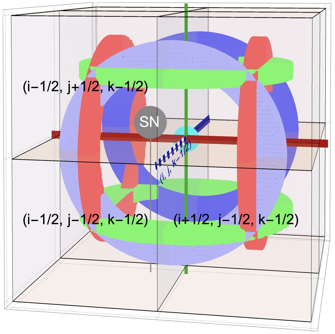
We select the orientation of the loop (and therefore, the respective set of signs in Equation 4 as a function of the local magnetic field in such a way that the injection maximises the amount of magnetic energy generated. This selection is made so that the injected energy matches the target injection energy. When a simple injection configuration is selected, there is no guarantee that at least a part of the injected magnetic field will not oppose the pre-existing magnetic field. As a result, the amount of injected energy in each event is not fixed, but oscillates around the desired value. In our simulations, we aim to inject a magnetic energy . Fig. 13 shows the average injected magnetic energy in the three runs with injection as a function of redshift. The desired energy is represented by the horizontal dashed gray line. Overall, all our runs tend to inject a magnetic energy on the desired order of magnitude. We note that the B20SN simulation has a slightly higher injection efficiency, which is due to the initial absence of magnetic fields, and therefore the selected injection geometry opposing a smaller fraction of the local field. Finally, we note that our selection for the direction of the injection will have a slight preference to align the injected field with any existing field, as this maximises the injected energy. As a result, injections will tend to positive cross-term instead of negative cross-term magnetic energy when separated by the magnetic tracers.