Statistical and computational thresholds for the planted $k$ -densest sub-hypergraph problem

Luca Corinzia, and Paolo Penna Affiliation: Department of Computer Science
ETH Zürich, Switzerland
Email: {luca.corinzia,paolo.penna}@inf.ethz.ch Wojciech Szpankowski Affiliation: Department of Computer Science
Purdue University, USA
Email: szpan@purdue.edu Joachim M. Buhmann Affiliation: Department of Computer Science
ETH Zürich, Switzerland
Email: jbuhmann@inf.ethz.ch

Abstract

In this work, we consider the problem of recovery a planted $k$ -densest sub-hypergraph on $d$ -uniform hypergraphs. This fundamental problem appears in different contexts, e.g., community detection, average-case complexity, and neuroscience applications as a structural variant of tensor-PCA problem. We provide tight information-theoretic upper and lower bounds for the exact recovery threshold by the maximum-likelihood estimator, as well as algorithmic bounds based on approximate message passing algorithms. The problem exhibits a typical statistical-to-computational gap observed in analogous sparse settings that widen with increasing sparsity of the problem. The bounds show that the signal structure impacts the location of the statistical and computational phase transition that the known existing bounds for the tensor-PCA model do not capture. This effect is due to the generic planted signal prior that this latter model addresses.

I Introduction

High dimensional inference problems play a key role in recent machine learning and data analysis applications. Typical scenarios exhibit problem dimensions comparable to the sample size, hence precluding effective estimation with no further structure imposed on the underlying signal, such as low-rank or sparsity. Most of these problems, as sparse mean estimation, compress sensing, low-rank matrix estimation, and planted clique estimation can be regarded as the general problem of recovery a planted signal when the available observations are perturbed by noise.

In this work we study the problem of recovery a planted $k$ -densest sub-hypergraph on $d$ -uniform hypergraph over $p$ nodes. This problem, considered in [1], is closely related to several community detection models and to the tensor-PCA. It addresses high order interactions described by hyperedges between nodes, that arise naturally in several applications, including brain region modeling [2, 3, 4] and memory [5], computer vision applications [6], and network analysis [7, 8, 9].

The planted solution consists of a subset of $k$ randomly chosen nodes out of $p$ . The weights of all $\binom{k}{d}$ uniform hyperedges inside the planted solution have a bias $\beta$ . The weights of all hyperedges are then perturbed with Gaussian noise, and the problem consists in detecting the necessary signal-to-noise ratio (snr) such that it is possible to recover the planted set given the noisy observations.

In this paper, we study information-theoretic (IT) and computational algorithmic limits for this class of recovery problems, given by the parameters $d$ , $k$ and $p$ . In particular, we are interested in the existence of the so-called statistical-to-computational (SC) gaps in the sparse regime $k\in o(p)$ .

I-A Contribution

We here summarize the two main contributions given in this paper.

(i) We provide upper and lower bounds on the recoverability threshold according to the vectorial maximum-likelihood estimator (that is generally non-tractable). These thresholds are located at finite values according to a rescaled snr $\gamma$ defined in Equation 5, and are hence almost tight compared to previous bounds in [1]. The upper bound is based on a union bound analysis, see Theorem 1. The lower bound is a major technical contribution as it requires to address the dependencies between solution weights. The analysis is performed with two main arguments according to different regimes: recent tail bounds for the maximum of Gaussian r.v. with bounded correlation in Theorem 2 and the generalized Fano’s inequality in Theorem 3, both combined with a classic covering argument from information theory. For $d\to+\infty$ , the lower bound matches the IT threshold provided recently in [10] for the tensorial MMSE estimator.

(ii) We provide a heuristic derivation of approximate-message-passing (AMP) algorithm for our problem, together with a state evolution analysis. The derivation generalizes the tensor-PCA AMP algorithm with a non-factorizable prior distribution. The recovery threshold for this class of algorithms is reported in 1.

I-B Related Work

The study of the recovery of a planted signal in a probabilistic generative model has received much attention recently, as it constitutes a fertile ground for the analysis of the SG gaps. Many variations of the planted problem have been addressed in the literature. The stochastic block model for community detection in graphs [11, 12, 13] or hypergraphs [14, 15]) has been one of the first model to be studies and does not present any SC gap [11, 16]. Despite these models have been mainly used with discrete Bernulli random variables, recent extension to weighted edges have been proposed (see [17, 18]). Analogously, the dense matrix-PCA problem [19, 20] has been shown not to have any SC gap, as the proposed AMP algorithms match the statistical thresholds [20].

SC gaps have been first observed in the context of dense tensor-PCA [21, 22, 23, 24, 25, 26] and recently in the sparse matrix [27] and tensor extension [10, 28]. The last two works address only the statistical phase transition and are described in detail as the closest to our work. In [10], the statistical threshold for the MMSE estimator is fully characterized for the sparse tensor-PCA problem, and it is shown that the estimator undergoes an all-or-nothing transition. After proper rescaling, the snr threshold given in [10] for the MMSE estimator is located exactly at the lower bound threshold here proved in Theorem 2. The characterization is, however, performed for the tensorial (multi-dimensional) MMSE estimator. This estimator is allowed to return any tensor in the unit ball, with no guarantee whether this can be used to recover the vectorial planted signal. Moreover, the precise relation between the MMSE and the MLE here addressed is generally still unknown, as mentioned in [10]. Indeed, [28] showed that a stronger condition on the MMSE behaviour produces an equivalent transition on the tensorial MLE, which imposes limitations on the sparsity regime for which the results apply.

Other results on tensor-PCA bounds [21, 22, 23] with generic signal prior are not tight in most of the cases if applied to our problem in a black-box fashion (see, e.g. the comparison with prior upper and lower bounds given in Section D-A). This is due to the specific combinatorial structure of the planted vector (that is, in turn, a restriction on the signal prior) that is not specified for the generic spherical prior tensor-PCA.

Regarding the computational thresholds, the algorithm here described is an extension of the tensor-PCA AMP algorithm to sparse hypergraph settings. These algorithms have been shown to be information-theoretic optimal in numerous high dimensional statistical estimation problems (dense matrix-PCA [20], SBM [29] etc.) and to outperform other class of algorithms in the case of SC gaps (see e.g., planted clique problem [30] and sparse matrix-PCA [27]). Nonetheless, AMP algorithms have been shown to underperform in the tensor-PCA problem [31] to the sum-of-squares class [22] and recently to averaged gradient descent [32]. However, a recent work suggests that a hierarchy of such AMP algorithms may actually match the performance of the best known efficient algorithms [33].

II Setting

We study the problem of recovery a planted sub-hypergraph on a $d$ -uniform hypergraph over $p$ nodes. Every subset of $d$ nodes $\{i_{1},i_{2},\ldots,i_{d}\}$ is an hyperedge whose weight $Y_{i_{1},i_{2},\ldots,i_{d}}$ is a Gaussian random variable, defined according to the following process. We denote by $\mathbf{x}\in\mathcal{C}_{p,k}\subset\{0,1\}^{p}$ the vector of selected nodes, with

\mathcal{C}_{p,k}\coloneqq\{\mathbf{x}\in\{0,1\}^{p}\colon\sum_{i}x_{i}=k\}.

Furthermore, we assume that $\mathbf{x}$ is drawn uniformly at random in $\mathcal{C}_{p,k}$ with probability $\mathbb{P}_{p}$ . The resulting weights are given by the $d$ -order tensor $\mathbf{Y}\coloneqq\mathbf{Y}(\mathbf{x})$ in which all edges indicated by $\mathbf{x}$ have a bias $\beta\geq 0$ , and the weights are perturbed by adding Gaussian noise across all hyperedges $(i_{1}i_{2}\cdots i_{d})$ with $i_{1}<i_{2}<\dots<i_{d}$ . For convenience let us now introduce the following tensor notation. The outer product of two tensors $\mathbf{U}\in\bigotimes^{d_{1}}\mathbb{R}^{p}$ and $\mathbf{V}\in\bigotimes^{d_{2}}\mathbb{R}^{p}$ is denoted by $\mathbf{U}\otimes\bm{V}$ with entries $(\mathbf{U}\otimes\bm{V})_{i_{1}i_{2}\ldots i_{d_{1}}j_{1}j_{2}\cdots j_{d_{2}}}=\mathbf{U}_{i_{1}i_{2}\cdots i_{d_{1}}}\mathbf{V}_{j_{1}j_{2}\ldots j_{d_{2}}}$ . For $\bm{x}\in\mathbb{R}^{p}$ , we define $\bm{x}^{\otimes d}=\bm{x}\otimes\cdots\otimes\bm{x}\in\bigotimes^{d}\mathbb{R}^{p}$ as the $d$ -th outer power of $\bm{x}$ . The inner product of the two tensors $\mathbf{U}\in\bigotimes^{d_{1}}\mathbb{R}^{p}$ and $\mathbf{V}\in\bigotimes^{d_{2}}\mathbb{R}^{p}$ with $d_{2}\leq d_{1}$ is defined as $\langle\mathbf{U},\mathbf{V}\rangle=\sum_{j_{1},\ldots,j_{d_{2}}}\mathbf{U}_{i_{1},\ldots,i_{d_{2}-d_{1}},j_{1},\ldots,j_{d_{2}}}\mathbf{V}_{j_{1},\ldots,j_{d_{2}}}.$ Given a $d$ -th order tensor $\mathbf{U}\in\bigotimes^{d}\mathbb{R}^{p}$ , we define the map $\mathbf{U}:\mathbb{R}^{p}\to\mathbb{R}^{p}$ as

\displaystyle\bm{U}\{\bm{x}\}_{i}=\sum_{i_{2},\ldots,i_{d}}U_{i,i_{2},\ldots,i_{d}}\ x_{i_{2}}\cdot\ldots\cdot x_{i_{d}}.

(1)

Using tensor notation, the observation model reads:

\displaystyle\mathbf{Y}=(\beta\mathbf{x}^{\otimes d}+\mathbf{Z})\mathbbm{1}_{\{i_{1}<\dots<i_{d}\}}

(2)

where $\mathbbm{1}_{\{P\}}=1$ if $P$ is true, and $0$ otherwise, and $Z_{i_{1}i_{2}\cdots i_{h}}\sim\mathcal{N}(0,1)$ . Note the main difference with the tensor-PCA formulation of the problem, where all the elements of the tensor are observed. For any signal $\mathbf{x}$ , we also consider the sum of all $\binom{k}{d}$ weights of the hyperedges with nodes in $\mathbf{x}$ as:

	$\displaystyle S(\mathbf{x})$	$\displaystyle\coloneqq\sum_{i_{1}<i_{2}<\ldots<i_{d}}Y_{i_{1},i_{2}\ldots,i_{d}}x_{i_{1}}\cdot x_{i_{2}}\dots\cdot x_{i_{d}}$
		$\displaystyle=\sum_{i}\mathbf{Y}\{\mathbf{x}\}_{i}=\langle\mathbf{Y},\mathbf{x}^{\otimes d}\rangle$		(3)

Definition 1 (Partial and exact receovery).

A $k^{\prime}$ -partial recovery is achieved if there exists an estimator $\hat{\mathbf{x}}$ that, with input the weight tensor $\mathbf{Y}(\mathbf{x})$ given by (2), returns $\hat{\mathbf{x}}=\hat{\mathbf{x}}(\mathbf{Y})$ such that

\mathbb{P}(\langle\hat{\mathbf{x}},\mathbf{x}\rangle\geq k^{\prime})=1-o(1).

Exact recovery is achieved if

\mathbb{P}(\langle\hat{\mathbf{x}},\mathbf{x}\rangle=k)=\mathbb{P}(\hat{\mathbf{x}}=\mathbf{x})=1-o(1).

Definition 2 (Maximum-likelihood estimator).

The vectorial maximum-likelihood estimator is defined as

\mathbf{x}_{\MLE}(\mathbf{Y})=\argmax\limits_{\hat{\mathbf{x}}\colon\mathbf{Y}\to\hat{\mathbf{x}}(\mathbf{Y})\in\mathcal{C}_{p,k}}\mathbb{P}(\mathbf{Y}|\hat{\mathbf{x}(\mathbf{Y})})

We define as $P_{r}^{(k^{\prime})}=\mathbb{P}(\langle\mathbf{x}_{\MLE},\mathbf{x}\rangle\geq k^{\prime})$ and $P_{r}$ accordingly.

It is easy to see that the vectorial MLE estimator for the problem in Equation 2 corresponds to the $k$ -densest sub-hypergraph (from this the name of the problem, see Theorem 4 in [1] for a proof)

	$\displaystyle\mathbf{x}_{\MLE}(\mathbf{Y})$	$\displaystyle=\argmax\limits_{\hat{\mathbf{x}}\colon\mathbf{Y}\to\hat{\mathbf{x}}(\mathbf{Y})\in\mathcal{C}_{p,k}}\sum_{i_{1}<\dots<i_{d}}Y_{i_{1},\dots,i_{d}}\hat{x}_{i_{1}}\cdot\dots\cdot\hat{x}_{i_{d}}$
		$\displaystyle\hskip-28.45274pt=\argmax\limits_{\hat{\mathbf{x}}\colon\mathbf{Y}\to\hat{\mathbf{x}}(\mathbf{Y})\in\mathcal{C}_{p,k}}\langle\mathbf{Y},\hat{\mathbf{x}}^{\otimes d}\rangle=\argmax\limits_{\hat{\mathbf{x}}\colon\mathbf{Y}\to\hat{\mathbf{x}}(\mathbf{Y})\in\mathcal{C}_{p,k}}S(\hat{\mathbf{x}})$		(4)

Our bounds depend on the scale-normalized snr:

\gamma\coloneqq\beta\sqrt{\frac{\binom{k}{d}}{k}\cdot\frac{1}{2\log p}}.

(5)

This scaling incorporates the parameters $k$ and $d$ of the problem and it will result in information-theoretic thresholds located at finite values.

Remark 1.

The scale-normalized snr $\gamma$ in Equation 5 can be seen as the effective snr of the problem, given by total signal / total noise. The total signal is $\beta$ , times the number of planted edges, hence $\beta\binom{k}{d}$ . The total noise is the standard deviation $\sqrt{\binom{k}{d}}$ times the scale of the number of solutions $\sqrt{2\log\binom{p}{k}}\approx\sqrt{2k\log p}$ . The latter rescale has the following intuitive justification. If we assume that $\binom{p-k}{k}\approx\binom{p}{k}$ unbiased solutions are independent, then their maximum is located at $\sqrt{\binom{k}{d}}\sqrt{2\log p}$ . The total signal has then to exceed this quantity, in order for the recovery to be possible. This argument ignores the dependencies between solutions, but it provides the right scaling of the snr.

Note that all these parameters may depend on $p$ , that is, we consider $k=k_{p}$ and $d=d_{p}$ . Throughout the paper, we hide the dependency on $p$ for readability. In most of the analysis, the following rescaling of the involved quantities will appear naturally

\alpha_{q}\coloneqq\lim_{p\rightarrow+\infty}\frac{\log q}{\log p}

(6)

which intuitively means that $q\approx n^{\alpha_{q}}$ . We call $\alpha_{q}$ the rate of a generic $q=q_{p}$ .

III Information-Theoretic Bounds

By the MLE estimator’s characterisation given in Section II, the recovery regime is regulated by the weight $S(\mathbf{x})$ of the planted solution and how it compares to the best among all other solutions’ weights. For the analysis, it is useful to partition the latter according to their overlap with the planted solution.

Lemma 1.

For any $m\in\{0,\ldots,k\}$ , let

\mathcal{S}_{m}=\{\hat{\mathbf{x}}\in\mathcal{C}_{p,k}\colon\langle\mathbf{x},\hat{\mathbf{x}}\rangle=m\}

denote the set of all solutions that share exactly $m$ nodes with the planted solution $\mathbf{x}$ . Then the following bound holds for all $k^{\prime}\in\{0,\ldots,k\}$ :

\displaystyle 1-P_{r}^{(k^{\prime})}

\displaystyle\leq\sum_{m=0}^{k^{\prime}-1}\mathbb{P}\left(S(\mathbf{x})<\max_{\hat{\mathbf{x}}\in\mathcal{S}_{m}}S(\hat{\mathbf{x}})\right).

(7)

For all $m<k$ it further holds:

\displaystyle 1-P_{r}

\displaystyle\geq\mathbb{P}\left(S(\mathbf{x})<\max_{\hat{\mathbf{x}}\in\mathcal{S}_{m}}S(\hat{\mathbf{x}})\right).

(8)

The proof of this lemma is given by a union bound and is given in the appendix. Given Definition 2 and the latter inequalities, we can reduce the analysis of the recovery regime to the determination of the values of $\gamma$ for which $\mathbb{P}\left(S(\mathbf{x})<\max_{\hat{\mathbf{x}}\in\mathcal{S}_{m}}S(\hat{\mathbf{x}})\right)$ vanishes or has limit 1, for $p\to+\infty$ . In the first scenario (recovery regime), these probabilities need to vanish sufficiently fast to apply the union bound in Equation 7 over all different $m$ .

III-A Upper bound (partial or exact recovery)

We here provide upper bounds on the failure probability of partial and exact recover. The proof is given in appendix.

Theorem 1.

For any $k$ and any $k^{\prime}\in\{1,\ldots,k\}$ , and for any $\gamma>\gamma^{({k^{\prime}})}_{\UB}$ , the MLE estimator achieves $k^{\prime}$ -partial recovery according to Definition 1. The critical gamma is defined as

\gamma^{({k^{\prime}})}_{\UB}\coloneqq\sqrt{1+\alpha_{k}-2\alpha_{k-k^{\prime}}+\alpha_{k^{\prime}}}+\sqrt{\alpha_{k}-\alpha_{k-k^{\prime}}+\alpha_{k^{\prime}}}

where $\alpha_{k}$ , $\alpha_{k^{\prime}}$ and $\alpha_{k-k^{\prime}}$ are defined according to Equation 6.

It follows easily from the latter theorem, the following on exact recovery.

Lemma 2.

Exact recovery is achieved for $\gamma>\gamma_{\UB}$ , with

\gamma_{\UB}=\sqrt{1+2\alpha_{k}}+\sqrt{2\alpha_{k}}.

Recovery of a constant fraction of $k$ nodes is achieved with $k^{\prime}=\lambda k$ , with $\lambda$ constant, for $\gamma>\gamma_{\UB}^{(\lambda k)}$ with

\gamma_{\UB}^{(\lambda k)}=1+\sqrt{\alpha_{k}}.

III-B Lower bounds (impossibility of recovery)

We here provide a characterisation of the regime where recovery is impossible, given by the following two theorems, valid in different regimes.

Theorem 2.

For $\alpha_{k}\in(0,1)$ , and for $d\in\omega(1)$ the following holds.

\lim_{p\to+\infty}P_{r}=0

for any $\gamma<\gamma_{\LB,\G}$ , with $\gamma_{\LB,\G}$ given by:

\displaystyle\gamma_{\LB,\G}\coloneqq\begin{cases}\sqrt{1-\alpha_{k}}&\text{ for }d\in o(\sqrt{k})\\ \sqrt{1-\alpha_{k}}/\sqrt{e}&\text{ otherwise }\end{cases}

(9)

Theorem 3.

For $\alpha_{k}\in(0,1)$ and any $d$ , the following holds.

\limsup\limits_{p\to+\infty}P_{r}<1

for any $\gamma<\gamma_{\LB,{\sf F}}$ , with $\gamma_{\LB,{\sf F}}$ given by:

\displaystyle\gamma_{\LB,{\sf F}}\coloneqq\sqrt{\frac{1-\alpha_{k}}{2}}

(10)

The first theorem gives tighter bounds, but its validity is confined to the case where the order of the hypergraph (or tensor) $d$ grows to infinity with $p$ . The second theorem is valid in any regime. However, it provides only an impossibility result as $\limsup P_{r}<1$ , and achieves a lower threshold. The proofs in the two regimes use two main arguments that are, respectively: (i) A recent tail bound on the maximum of dependent Gaussians with bounded correlation (see [34] and Lemma 10) and (ii) the generalised Fano’s inequality. Both proofs consider a coverage set of weakly overlapping solutions defined below. Intuitively, recovery in the original problem is at least as difficult as the recovery restricted to this set of weakly dependent solutions if the coverage is sufficiently large.

Definition 3.

For any $r\in\{0,\ldots,k\}$ define the coverage with overlap $r$ a subset $\mathcal{C}(r)\subset\mathcal{C}_{p,k}$ of solutions satisfying the following conditions: (i) Any two solutions in $\mathcal{C}(r)$ share less than $r$ nodes. (ii) For any solution $\mathbf{x}^{\prime}\in\mathcal{C}_{p,k},\mathbf{x}^{\prime}\not\in\mathcal{C}(r)$ there exists a solution $\mathbf{x}^{\prime\prime}\in\mathcal{C}(r)$ such that $\mathbf{x}^{\prime}$ and $\mathbf{x}^{\prime\prime}$ have at least $r$ nodes in common. We denote by $C(r)\coloneqq|\mathcal{C}(r)|$ the cardinality of the coverage.

In the proof of Theorem 2, we use the above mentioned result [34] to show that the maximum among solutions in $\mathcal{C}(r)$ concentrates tightly around $\sigma_{k}\sqrt{\alpha_{C(r)}\cdot 2\log p}$ where $\sigma_{k}=\sqrt{\binom{k}{d}}$ , while the planted solution concentrates around its expectation $\beta_{k}=\beta\binom{k}{d}$ . Then, the condition for recovery translates into $\beta_{k}>\sigma_{k}\sqrt{\alpha_{C(r)}\cdot 2\log p}$ which corresponds to $\gamma<\sqrt{\frac{\alpha_{C(r)}}{k}}$ . A crucial point is that, in order to prove the concentration of the maximum over $\mathcal{C}(r)$ , the overlap $r$ has to be small enough such that the maximum correlation between solutions weights $S(\hat{\mathbf{x}})$ vanishes, which gives the conditions on $d$ in Theorem 2 and the corresponding bound on $\alpha_{C(r)}$ .

The proof of Theorem 3 is based on Fano’s inequality. By restricting to the solutions in $\mathcal{C}(r)$ , we use the generalized Fano’s inequality [35] to show that $P_{r}$ satisfies the bound $P_{r}\lesssim 1-\I(\mathbf{x};\mathbf{Y})\cdot\log^{-1}C(r)$ where $\I(\mathbf{x};\mathbf{Y})$ is the mutual information between the planted solution $\mathbf{x}$ and the observations $\mathbf{Y}(\mathbf{x})$ . By using [35] and the combinatorial structure of $\mathcal{C}_{p,k}$ , we can upper bound the mutual information as $\binom{k}{d}\beta^{2}$ . The rescaling of $\gamma$ and a lower bound on the cardinality of the coverage set $C(r)$ gives the claim. The proof of both theorems is given in the appendix.

IV Computational Thresholds via Approximate Message Passing

Fig. 1: Empirical performance of the AMP algorithm for fixed

p=500

d=3

and different values of

k

(respectively, from left to right,

k=20,10,5

). The experiment is repeated 20 times, and we report the median overlap achieved. The AMP and AMP VECT refer respectively to using a scalar and a vectorial thresholding function as in Equation 13.

Refer to caption — Fig. 2: State evolution fixed point overlap $m^{*}$ reached by the factorized equation in Equation 14. The first row reports the overlap obtain with uninformative initialization (UI, $m_{0}\approx 0$ ), while the bottom row reports the overlap with informative initialization $m_{0}=1$ . The empirical fixed point with UI well matches the analytical AMP threshold given by 1 (brown line, expressed in terms of the $\beta$ parameter), while the II fixed point approaches the conjectured IT threshold located at the lower bound.

Approximate message passing algorithms are a class of algorithms for high dimensional statistical estimation that approximate belief propagation in the large system limit [36]. Intuitively, it iteratively estimates the mean $\bm{x}^{(t)}$ and the variance $\bm{a}^{(t)}$ of the classic belief propagation messages in the factor graph of the estimation problem, discarding low order terms that depend on the target factor node of the messages. The algorithm results in a slight modification of a general spectral algorithm for tensor-PCA. In the following, we use the operator ‘ $\circ$ ’ to denote an operation that is performed elementwise on a vector or tensor. Let introduce the following probability distribution

g(\bm{y}|\bm{a},\bm{x})=\frac{\mathbb{P}_{p}(\bm{y})\exp(\bm{x}\cdot\bm{y}-(\bm{y}\circ\bm{y})\cdot\bm{a})/2}{Z(\bm{a},\bm{x})}

where $Z(\bm{a},\bm{x})$ is the normalizing constant. Then, we define the following threshold function which will be used in the definition of AMP algorithm below:

f(\bm{a},\bm{x})=\mathbb{E}_{g(\cdot|\bm{a},\bm{x})}[y].

(11)

IV-A The AMP procedure

The iterative AMP procedure reads (derivation given in Appendix C):

		$\displaystyle\bm{b}^{(t)}=\beta^{2}(d-1)\langle\bm{Y}^{\circ 2},\bm{\sigma}^{(t)}\otimes(\bm{\hat{x}}^{(t)}\circ\bm{\hat{x}}^{(t-1)})^{\otimes d-2}\rangle$
		$\displaystyle\bm{x}^{(t)}=\beta\mathbf{Y}\{\bm{\hat{x}}^{(t)}\}-\langle\bm{b}^{(t)},\bm{\hat{x}}^{(t-1)}\rangle$
		$\displaystyle\bm{a}^{(t)}=\beta^{2}\bm{Y}^{\circ 2}\{\bm{(\hat{x}}^{(t)})^{\circ 2}\}$		(12)
		$\displaystyle\bm{\sigma}^{(t+1)}=\bm{diag}(\bm{J}_{x}f(\bm{a}^{(t)},\bm{\hat{x}}^{(t)}))$
		$\displaystyle\bm{\hat{x}}^{(t+1)}=f(\bm{a}^{(t)},\bm{x}^{(t)})$

where $\bm{J}_{x}f$ is the Jacobian w.r.t varible $x$ of the function $f$ and $\bm{diag}(\cdot)$ extracts its diagonal entries. The threshold function $f$ becomes tractable when the prior distribution $\mathbb{P}_{p}$ factorizes as $\mathbb{P}_{p}(\bm{x})=\prod_{i}p(x_{i})$ . In this case, the threshold function $f$ factorizes as well into independent components, and the AMP equations proposed here are equivalent to those in [31] (more details in Appendix C). In our problem, however, the prior distribution does not factorize since $\mathbb{P}_{p}$ is the uniform distribution over $\mathcal{C}_{p,k}$ . A similar issue arises in the planted clique problem studied in [30], where the authors propose to approximate the prior distribution with a factorized Bernulli distribution with parameter $\delta=k/p$ . With this approximation, the threshold function reads $f(\bm{a},\bm{x})=(f_{i}(a_{i},x_{i}))_{i=1}^{p}$ , where

\displaystyle f_{i}(a_{i},x_{i})=\frac{1}{1+\exp(-x_{i}+a_{i}/2+\log(1/\delta-1)}\ .

While this Bernulli approximation is effective for large $k$ – like the regime $k=\Theta(\sqrt{p})$ studied in [30] – it may be inaccurate for small $k$ . We indeed observe experimentally (see Section V) that for small values of $k$ , the above approximation is no longer effective. Hence, we propose a finer approximation of the threshold function that is still tractable. Our parametrization is inspired by the independent Bernoulli approximation:

f(\bm{a},\bm{x})=\left(\frac{1}{1+\exp(-x_{i}+a_{i}/2+\lambda(\bm{x})}\right)_{i=1}^{p}

(13)

with $\lambda(\bm{x})$ being a scalar used to enforce $f$ to select $k$ components equals to $1$ , hence given by $\sum_{i}f_{i}(\bm{a},\bm{x})=k$ . The experiments described in section V below show that our finer approximation outperforms the Bernulli i.i.d. approximation.

IV-B State Evolution

The evolution of the approximated message passing algorithm in the special case of Bayesian-optimal inference, can be tracked by a one dimensional iterative equation of the overlap order parameter. In our setting, with a generic (non-factorizable) prior distribution $\mathbb{P}_{p}$ and threshold function $f$ we can define the multidimensional overlap order parameter as

\bm{m}^{(t)}=\frac{1}{\binom{p-1}{d-1}}\mathbb{E}_{\bm{x}}[\bm{1}\{\bm{x}\circ\bm{x}^{(t)}\}]

where $\bm{1}$ is the tensor with components $\bm{1}_{i,i_{2},\dots,i_{d}}=1$ if $i_{2}<i_{3}<\dots<i_{d}$ and $0$ otherwise. The multidimensional state evolution (SE) (generalizing [31]) reads then (see Appendix C for a heuristic derivation):

\displaystyle\bm{m}^{(t+1)}=\frac{{\mathbb{E}}_{\bm{x},\bm{z}}\left[\bm{1}\{\bm{x}\circ f\left(\bm{\hat{m}}^{(t)},\bm{\hat{m}}^{(t)}\circ\bm{x}+(\bm{\hat{m}^{(t)}})^{\circ 1/2}\circ\bm{z}\right)\}\right]}{\binom{p-1}{d-1}}

where $\bm{\hat{m}}^{(t)}=\beta^{2}\binom{p-1}{d-1}\bm{m}^{(t)}$ and $\bm{z}$ is a $p$ -dimensional vector with i.i.d. standard Gaussian entries. Note again that assuming a factorized i.i.d. prior distribution $\mathbb{P}_{p}(\bm{x})=\prod_{i}p(x_{i})$ the SE is equivalent to the single letter evolution of the scalar overlap $m_{t}=\frac{1}{p}\langle\bm{x},\bm{\hat{x}}^{(t)}\rangle$ described in [31],

m_{t+1}=\mathbb{E}_{x,z}\left[x\cdot f(\hat{m}_{t},\hat{m}_{t}x+\sqrt{\hat{m}_{t}}z)\right],

(14)

where $x\sim p$ , $z\sim\mathcal{N}(0,1)$ , and $\hat{m}_{t}=\beta^{2}\binom{p-1}{d-1}m_{t}$ . In the following we derive an analytical threshold for the AMP algorithm to succeed, approximating the true prior distribution with a factorized Bernulli prior with parameter $\delta=\frac{k}{p}$ and using the simplified SE in Equation 14. A simple heuristic argument based on the study of the fixed points of the SE is given inAppendix C.

Claim 1.

The recovery threshold for the AMP algorithm reads:

\gamma_{\AMP}\coloneqq\sqrt{\frac{1}{2e}\left(\frac{p}{k}\right)^{d-1}\frac{1}{d(d-1)\log p}}.

(15)

V Experiments and Discussion

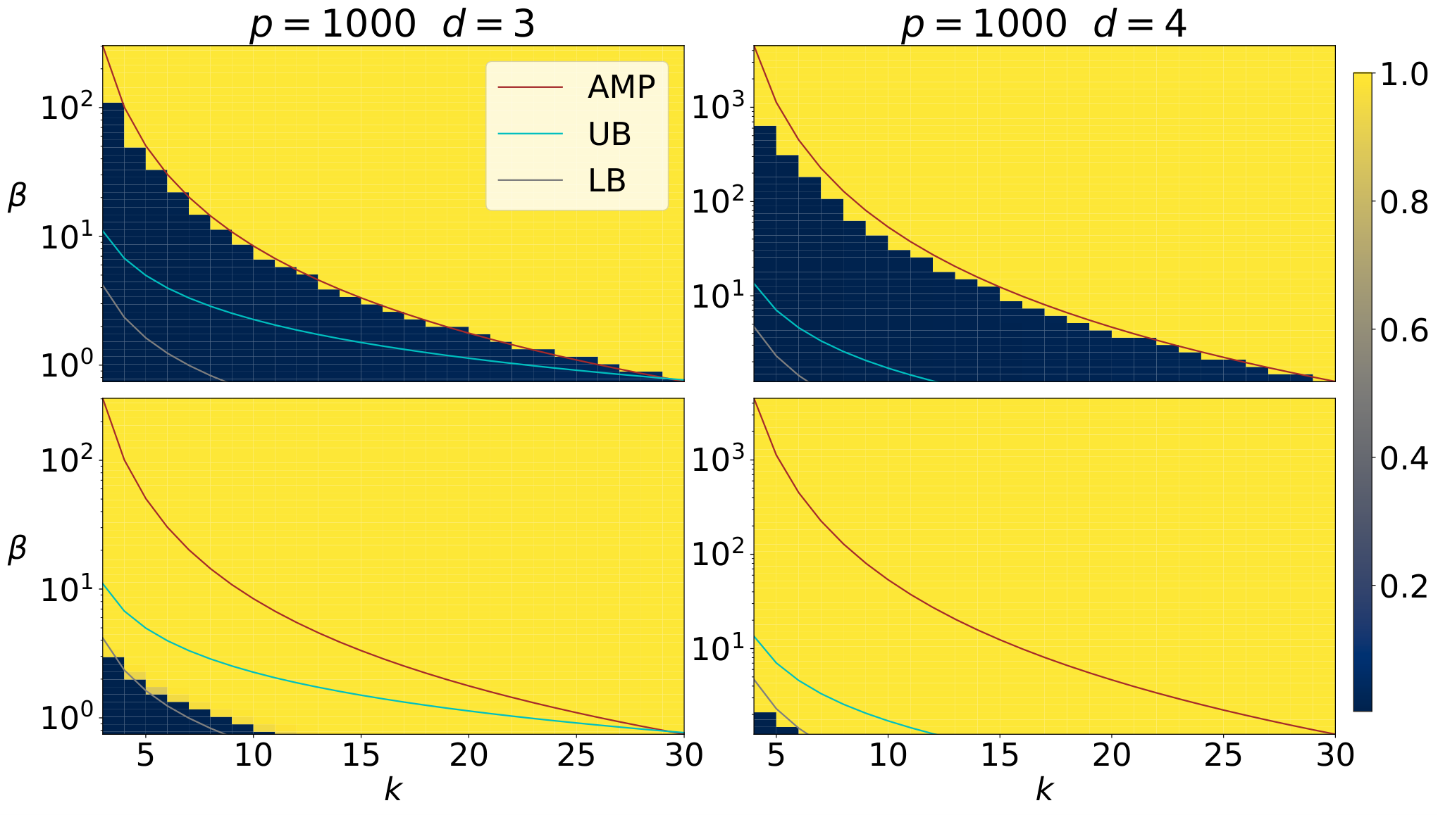
In Figure 1, we report both the empirical performance of the AMP algorithm and the factorized SE fixed point (according to Equation 14) for uninformative initialization (with a random overlap with the planted solution) and informative initialization (respectively UI and II) for different values of $k$ . For a high value of $k$ , the Bernoulli i.i.d. approximation of the prior function and factorized thresholding function well matches the SE fixed point, with the UI empirical performance slightly worse than the SE prediction due to finite-size effects (as already observed for the planted clique problem in graphs [30]). At smaller values of $k$ , the statistical dependency between signal components increases and the AMP empirical performance heavily mismatch the SE prediction. In this setting, the proposed multivariate threshold function significantly outperforms the naive factorized AMP, matching the SE in the II setting correctly. Interestingly, the dynamic phase transition of the AMP indicated by the critical signal at which the SE with II fails approaches the conjectured information-theoretic threshold $\gamma_{\LB}$ . This finding suggests a possibility of analysis of the IT thresholds with statistical physics-inspired techniques (e.g., interpolation methods [27]) that so far have never been applied rigorously to the case of structured priors in the sparse setting. In Figure 2 we also report the factorized SE fixed point for $d=3$ and $d=4$ for both UI and II. We can observe the good agreement between the analytical computational threshold given by 1 and the SE’s empirical fixed point. The dynamical phase transition indicated by the $m^{*}$ transition for II (bottom row) is close to the information-theoretic lower bound (as shown already for the tensor-PCA problem [31]).

Acknowledgement

This work was supported in part by NSF Center on Science of Information Grants CCF-0939370 and NSF Grants CCF-1524312, CCF-2006440, CCF-2007238.

Appendix A Postponed proofs

Proof of Lemma 1.

By definition of $P_{r}^{(k^{\prime})}$ , $1-P_{r}^{(k^{\prime})}=\mathbb{P}\left(\langle\mathbf{x}_{\MLE},\mathbf{x}\rangle<k^{\prime}\right)$ . By the characterization of the MLE in Section II and the definition of $\mathcal{S}_{m}$ , the latter event is equal to

\{S(\mathbf{x})>S(\hat{\mathbf{x}}),\ \forall\ \hat{\mathbf{x}}\in\mathcal{S}_{0}\cup\cdots\cup\mathcal{S}_{k^{\prime}-1}\}.

The claim in Equation 7 follows then from the union-bound on the probability

\mathbb{P}\left(\bigcup_{m=0}^{k^{\prime}-1}\left\{S(\mathbf{x})\leq\max_{\hat{\mathbf{x}}\in\mathcal{S}_{m}}(S(\hat{\mathbf{x}}))\right\}\right).

To prove the lower bound in Equation 8, we can observe that if $S(\mathbf{x})<\max_{\hat{\mathbf{x}}\in\mathcal{S}_{m}}(S(\hat{\mathbf{x}}))$ for some $m<k$ , then the $\mathbf{x}_{\MLE}\neq\mathbf{x}$ , and thus it fails to exactly recover the planted solution. ∎

A-A Proofs for the Lower Bound

Proof of Theorem 1.

For the analysis, we define the following quantities depending on $k^{\prime}\in\{0,\ldots,k-1\}$ (we consider $p,k,d$ to be the parameters of the problem, hence their dependency is not highlighted):

		$\displaystyle Q(k^{\prime})\coloneqq\binom{p-k}{k-{k^{\prime}}}$
		$\displaystyle M(k^{\prime})\coloneqq\binom{k}{k^{\prime}}\binom{p-k}{k-{k^{\prime}}}=\binom{k}{k-{k^{\prime}}}\binom{p-k}{k-{k^{\prime}}}$
		$\displaystyle D(k^{\prime})\coloneqq\binom{k}{d}-\binom{k^{\prime}}{d}.$

For each fixed subset of $k^{\prime}$ nodes of the planted solution, there are $Q(k^{\prime})$ solutions that share exactly these $k^{\prime}$ nodes with the planted solution. Moreover, there are exactly $M(k^{\prime})$ solutions that share any $k^{\prime}$ nodes with the planted solution. Each solution sharing $k^{\prime}$ nodes with the planted solution differs in $D(k^{\prime})$ edges with the latter. We use the union bound given in Equation 7, and control the quantities

\mathbb{P}\left(\max_{\hat{\mathbf{x}}\in\mathcal{S}_{m}}S(\hat{\mathbf{x}})>S(\mathbf{x})\right)

using the tail bounds of the Gaussian from Lemma 9 and spitting the inequality into the sum of two independent terms as in Lemma 11. We hence get the following Lemma (full proof given below in this section):

Lemma 3.

For every $\epsilon>0$ and for every $k^{\prime}<k$ and $k>1$ , let $\gamma^{(k^{\prime})}_{UB_{\epsilon}}\coloneqq\sqrt{\frac{\binom{k}{d}}{kD(k^{\prime})}}\cdot UB_{\epsilon}(k^{\prime})$ , where

\displaystyle UB_{\epsilon}(k^{\prime})\coloneqq\sqrt{\frac{\log M(k^{\prime})}{\log p}+\epsilon}+\sqrt{\frac{\log\binom{k}{k^{\prime}}}{\log p}+\epsilon}\ .

(16)

Then, for any $\gamma>\gamma^{({k^{\prime}})}_{UB_{\epsilon}}$ it holds that

\mathbb{P}\left(\max_{\hat{\mathbf{x}}\in\mathcal{S}_{k^{\prime}}}S(\hat{\mathbf{x}})>S(\mathbf{x})\right)\leq\frac{1}{\sqrt{\pi}p^{\epsilon}}.

Plugging the result of the latter Lemma into Equation 7 we get:

1-P_{r}^{(k^{\prime})}\in\mathcal{O}\left(\frac{k^{\prime}}{p^{\epsilon}}\right)\ .

Using now Lemma 16 to characterize further the bound $\gamma^{({k^{\prime}})}_{UB_{\epsilon}}$ , and reparametrazing $\epsilon=\alpha_{k^{\prime}}+\tilde{\epsilon}$ , with $\tilde{\epsilon}>0$ an arbitrarily constant, we have

\frac{k^{\prime}}{p^{\epsilon}}=\frac{k^{\prime}}{p^{\alpha_{k^{\prime}}}}\cdot\frac{1}{p^{\tilde{\epsilon}}}=\exp\left(\log p\left[-\tilde{\epsilon}+\frac{\log k^{\prime}}{\log p}-\alpha_{k^{\prime}}\right]\right)\in o(1).

The asymptotics is due to the fact that $\frac{\log k^{\prime}}{\log p}-\alpha_{k^{\prime}}\rightarrow 0$ , by definition of $\alpha_{k^{\prime}}$ in Equation 6, and hence the expression $-\tilde{\epsilon}+\frac{\log k^{\prime}}{\log p}-\alpha_{k^{\prime}}$ is negative for sufficiently large $p$ . Hence, the probability $1-P_{r}^{(k^{\prime})}$ tends to $0$ . ∎

Proof of Lemma 3.

For an arbitrary subset $F$ of ${k^{\prime}}$ nodes of the planted solution $\mathbf{x}$ , denoted by $\mathbf{x}_{F}$ , with ${k^{\prime}}\in\{0,\ldots,k-1\}$ , let $\mathcal{S}_{k^{\prime}}^{F}$ be the set of all solutions that share exactly the set $F$ with the planted solution. Let $S^{-F}(\hat{\mathbf{x}})$ denote the sum of the weights in $\hat{\mathbf{x}}$ but not in $\mathbf{x}_{F}$ , as

S^{-F}(\hat{\mathbf{x}})=S(\hat{\mathbf{x}})-S(\hat{\mathbf{x}}\circ\mathbf{x}_{F}).

By the union bound over the $\binom{k}{k^{\prime}}$ possible fixed subsets $F$ of $k^{\prime}$ nodes, we get

$\displaystyle\mathbb{P}\left(\max_{\hat{\mathbf{x}}\in\mathcal{S}_{k^{\prime}}}S(\hat{\mathbf{x}})>S(\mathbf{x})\right)$	$\displaystyle\leq$
	$\displaystyle\hskip-28.45274pt\leq\binom{k}{{k^{\prime}}}\mathbb{P}\left(\max_{\hat{\mathbf{x}}\in\mathcal{S}_{k^{\prime}}^{F}}S(\hat{\mathbf{x}})>S(\mathbf{x})\right)$
	$\displaystyle\hskip-28.45274pt=\binom{k}{{k^{\prime}}}\mathbb{P}\left(\max_{\hat{\mathbf{x}}\in\mathcal{S}_{k^{\prime}}^{F}}S^{-F}(\hat{\mathbf{x}})>S^{-F}(\mathbf{x})\right)$	(17)

where the equality follows from subtracting from both sides the quantity $S(\mathbf{x}_{F})$ . Using Lemma 11, we have

$\displaystyle\mathbb{P}\left(\max_{\hat{\mathbf{x}}\in\mathcal{S}_{k^{\prime}}^{F}}S^{-F}(\hat{\mathbf{x}})>S^{-F}(\mathbf{x})\right)$	$\displaystyle\leq$
	$\displaystyle\hskip-85.35826pt\leq\mathbb{P}\left(\max_{\hat{\mathbf{x}}\in\mathcal{S}_{k^{\prime}}^{F}}S^{-F}(\hat{\mathbf{x}})>t\right)+\mathbb{P}\left(t\geq S^{-F}(\mathbf{x})\right)$
	$\displaystyle\hskip-85.35826pt\leq\mathbb{P}\left(\max_{\hat{\mathbf{x}}\in\mathcal{S}_{k^{\prime}}^{F}}S^{-F}(\hat{\mathbf{x}})>t_{\Delta^{\prime}}\right)+$
	$\displaystyle\hskip-28.45274pt+\mathbb{P}\left(D(k^{\prime})\beta-t_{\Delta^{\prime\prime}}>S^{-F}(\mathbf{x})\right)$
	$\displaystyle\hskip-85.35826pt\leq Q(k^{\prime})p(k^{\prime},\Delta^{\prime})+p(k^{\prime},\Delta^{\prime\prime})$	(18)

where the second inequality follows from Lemma 15 (together with the definition of $t_{\Delta^{\prime}}$ and $t_{\Delta^{\prime\prime}}$ ) and the latter inequality follows from Equation 30 and Equation 29 in Lemma 14. Combining Equation 17 and Section A-A, we get

	$\displaystyle\mathbb{P}\left(\max_{\hat{\mathbf{x}}\in\mathcal{S}_{k^{\prime}}}S(\hat{\mathbf{x}})>S(\mathbf{x})\right)$	$\displaystyle\leq\binom{k}{k^{\prime}}\left(Q(k^{\prime})p(k^{\prime},\Delta^{\prime})+p(k^{\prime},\Delta^{\prime\prime})\right)$
		$\displaystyle\hskip-99.58464pt=\binom{k}{k^{\prime}}\frac{1}{\sqrt{4\pi\log p}}\left(\left(\frac{1}{p}\right)^{\frac{\Delta^{\prime}}{D(k^{\prime})}}\frac{Q(k^{\prime})}{\sqrt{\Delta^{\prime}}}+\left(\frac{1}{p}\right)^{\frac{\Delta^{\prime\prime}}{D(k^{\prime})}}\frac{1}{\sqrt{\Delta^{\prime\prime}}}\right)$
		$\displaystyle\hskip-99.58464pt=\frac{1}{\sqrt{4\pi\log p}}\Bigg(\left(\frac{1}{p}\right)^{\frac{\Delta^{\prime}}{D(k^{\prime})}-\frac{\log M(k^{\prime})}{\log p}}\frac{1}{\sqrt{\Delta^{\prime}}}+$
		$\displaystyle\hskip-14.22636pt+\left(\frac{1}{p}\right)^{\frac{\Delta^{\prime\prime}}{D(k^{\prime})}-\frac{\log\binom{k}{k^{\prime}}}{\log p}}\frac{1}{\sqrt{\Delta^{\prime\prime}}}\Bigg)$

where in the first equality we used Equation 28 and in the last equality the identity $z=p^{\frac{\log z}{\log p}}$ and the fact that

\binom{k}{d}Q(k^{\prime})=\binom{k}{d}\binom{p-k}{k-k^{\prime}}=M(k^{\prime}).

Then, by Lemma 15, we get

	$\displaystyle\mathbb{P}\left(\max_{\hat{\mathbf{x}}\in\mathcal{S}_{k^{\prime}}}S(\hat{\mathbf{x}})>S(\mathbf{x})\right)$	$\displaystyle\leq\frac{1}{p^{\epsilon}}\frac{1}{\sqrt{4\pi\log p}}\left(\frac{1}{\sqrt{\Delta^{\prime}}}+\frac{1}{\sqrt{\Delta^{\prime\prime}}}\right)$
		$\displaystyle\hskip-56.9055pt\leq\frac{1}{p^{\epsilon}}\frac{1}{\sqrt{4\pi\log p}}\frac{1}{D(k^{\prime})}\Bigg(\sqrt{\frac{\log p}{\log M(k^{\prime})}}+$
		$\displaystyle\hskip 56.9055pt+\sqrt{\frac{\log p}{\log\binom{k}{k^{\prime}}}}\Bigg)$
		$\displaystyle\hskip-56.9055pt\leq\frac{1}{\sqrt{\pi}p^{\epsilon}}$

where in the last inequality we used $D(k^{\prime})\geq 1$ , $M(k^{\prime})\geq\binom{k}{k^{\prime}}\geq k$ , and $\log k>1$ , that valid for $k>k^{\prime}$ and $k>1$ . ∎

A-B Proofs of the Lower Bound

Proof of Theorem 2.

The proof of this lower bound is based on the result on tail bounds on the maximum of Gaussians with bounded correlation [34] given for convenience in Lemma 10. We here outline a road map of the proof: (i) Given an overlap $r\leq k$ between two solutions $\mathbf{x}^{\prime},\mathbf{x}^{\prime\prime}$ , we define the correlation $\rho(r)$ as the correlation between the random variables $S(\mathbf{x}^{\prime})$ and $S(\mathbf{x}^{\prime\prime})$ . We first analyze the conditions for vanishing correlation $\rho(r)\rightarrow 0$ . (ii) Using the tail bound on correlated Gaussians in Lemma 10, we show that vanishing correlation implies the concentration of the maximum of a given coverage of solutions $\mathcal{C}(r)$ . (iii) Using a lower bound on the rate of the cardinality of the coverage, we provide a respective lower bound of the recovery threshold. We hence first give a Lemma that characterizes the condition to have vanishing correlations.

Lemma 4.

For any two solutions $\mathbf{x}^{\prime},\mathbf{x}^{\prime\prime}\in\mathcal{C}_{p,k}$ , that share $r$ nodes as $\langle\mathbf{x}^{\prime},\mathbf{x}^{\prime\prime}\rangle=r$ , the correlation of the weights $\rho\coloneqq\rho_{S(\mathbf{x}^{\prime}),S(\mathbf{x}^{\prime\prime})}$ reads

\rho=\frac{\binom{r}{d}}{\binom{k}{d}}

and it vanishes in each of the following two regimes:

1.

For $d\in\omega(1)$ and $r\leq\lambda k$ for any constant $\lambda$ satisfying

$\displaystyle\begin{cases}\lambda<1&\text{ for }d\in o(\sqrt{k})\\ \lambda<1/e&\text{ otherwise }\end{cases}$ (19)
2.

For $d\in\mathcal{O}(1)$ and for any $r\in o(k)$ .

We can hence show in the following that, given a coverage with vanishing correlation $\rho(r)$ , the maximum of such coverage in bounded from below in high probability.

Lemma 5.

Given a number of shared nodes $r$ and a coverage $\mathcal{C}(r)$ that satisfies Definition 3, if the correlation between the weights of two solutions $\mathbf{x}^{\prime},\mathbf{x}^{\prime\prime}\in\mathcal{C}(r)$ , $\rho(r)=\rho_{S(\mathbf{x}^{\prime}),S(\mathbf{x}^{\prime\prime})}\to 0$ vanishes, then for any constant $\epsilon\in(0,1)$ the following upper bound on the maximum weight in the coverage holds:

\displaystyle\lim_{p\to+\infty}\mathbb{P}\left(\max_{\hat{\mathbf{x}}\in\mathcal{C}(r)}S(\hat{\mathbf{x}})\leq(1-\epsilon)\cdot\sigma_{k}\sqrt{\alpha_{C(r)}\cdot 2\log p}\right)=0

(20)

where $\sigma_{k}=\sqrt{\binom{k}{d}}$ .

We further provide a bound on the opposite direction for the weight of the planted solution, such that the two quantities can be well separated in high probability.

Lemma 6.

For any sequence $\Delta=\Omega\left(\frac{\binom{k}{d}}{\log p}\right)$ , it holds that

\displaystyle\lim_{p\to+\infty}\mathbb{P}_{z}\left(S(\mathbf{x})>\beta_{k}+\sqrt{\Delta\cdot 2\log p}\right)=0

where $\beta_{k}=\binom{k}{d}\beta$ and $\mathbf{x}$ is the planted solution.

We can prove the main Lemma that connects the recovery threshold to the rate of any coverage $\alpha_{C(r)}$ .

Lemma 7.

Given the assumptions of Lemma 5 and given that $\alpha_{C(r)}\in\Omega(1)$ , for any $\epsilon>0$ constant, if $\gamma\leq(1-\epsilon)\sqrt{\frac{\alpha_{C(r)}}{k}}$ , then the probability of recovery vanishes:

\displaystyle\lim_{p\to+\infty}P_{r}=0\ .

Proof.

From the hypothesis that $\alpha_{C(r)}\in\Omega(1)$ , $\log p\to+\infty$ , and given any constant $\delta_{0}>0$ the condition on $\gamma$ above implies that for $p$ large enough:

\gamma\leq(1-\epsilon)\sqrt{\frac{\alpha_{C(r)}}{k}}-\sqrt{\frac{\delta_{0}}{k\log p}}\ .

Using the definition of $\gamma$ and defining $\Delta=\delta_{0}\cdot\frac{\binom{k}{d}}{\log p}$ we get with simple manipulation:

\displaystyle(1-\epsilon)\sqrt{\binom{k}{d}}\sqrt{\alpha_{C(r)}\cdot 2\log p}>\binom{k}{d}\beta+\sqrt{\Delta\cdot 2\log p}

(21)

Using Lemma 11 and Equation 8, we can write an upper-bound on the recovery probability as:

	$\displaystyle P_{r}$	$\displaystyle\leq\mathbb{P}\left(\max_{\hat{\mathbf{x}}\in\mathcal{C}(r)}S(\hat{\mathbf{x}})\leq S_{\sf planted}\right)$
		$\displaystyle\leq\mathbb{P}\left(\max_{\hat{\mathbf{x}}\in\mathcal{C}(r)}S(\hat{\mathbf{x}})\leq t\right)+\mathbb{P}\left(t<S(\mathbf{x})\right).$

We can now use the condition in Equation 21, to get a $t$ such that the conditions for both Lemma 5 and Lemma 6 are satisfied. We hence obtain

\displaystyle\mathbb{P}\left(\max_{\hat{\mathbf{x}}\in\mathcal{C}(r)}S(\hat{\mathbf{x}})>t\right)\rightarrow 1

and

\displaystyle\mathbb{P}\left(S(\mathbf{x})\leq t\right)\rightarrow 1

(22)

and so the claim follows. ∎

Consider any $r=\lambda k$ with $\lambda$ being any constant satisfying Equation 19, according to the regime of $d$ and $k$ . By Lemma 4 and the assumption of the theorem $d\in\omega(1)$ , the correlation $\rho(r)$ vanishes. We can hence bound the recovery threshold with a respective bound on the rate $\alpha_{C(r)}$ , that is given in the following Lemma.

Lemma 8.

There exist a coverage $\mathcal{C}(r)$ according to Definition 3 with cardinality $\mathcal{C}(r)$ , $C(r)\coloneqq|\mathcal{C}(r)|$ at least

\displaystyle C(r)\gtrsim\frac{\binom{p}{k}}{B(r)}

for

\displaystyle B(r)=\sum_{l=r}^{k}\binom{k}{l}\binom{p-k}{k-l}.

(23)

For any $\alpha_{k}\in(0,1)$ and $r\leq\lambda k$ , with constant $\lambda\in(0,1)$ , and for $r\in\omega(\frac{k}{\log n})$ it holds that $\alpha_{C(r)}\gtrsim r(1-\alpha_{k})$ .

We can thus apply Lemma 7 and Lemma 8 with $r=\lambda k$ and obtain the desired result as follows:

(1-\epsilon)\sqrt{\frac{\alpha_{C(r)}}{k}}\geq(1-\epsilon)\sqrt{\lambda(1-\alpha_{k})}>\gamma

where the last inequality follows from the condition on $\gamma$ in Equation 9 and the hypothesis that $\lambda$ satisfies Equation 19. The above inequality and Lemma 7 implies the claim. ∎

Proof of Lemma 4.

Both $S(\mathbf{x}^{\prime})$ and $S(\mathbf{x}^{\prime\prime})$ are Gaussian random variables $\mathcal{N}(\mu,\beta^{2}\binom{k}{d})$ , where $\mu$ is the mean, and depends on the amount of nodes that the solution shares with the planted one $\mathbf{x}$ . The correlation is hence

\rho=\frac{{\mathbb{E}}[(S(\mathbf{x}^{\prime})-{\mathbb{E}}S(\mathbf{x}^{\prime}))(S(\mathbf{x}^{\prime\prime})-{\mathbb{E}}S(\mathbf{x}^{\prime\prime}))]}{\beta^{2}\binom{k}{d}}.

Observe that $S(\mathbf{x}^{\prime})-{\mathbb{E}}S(\mathbf{x}^{\prime})$ and $S(\mathbf{x}^{\prime\prime})-{\mathbb{E}}S(\mathbf{x}^{\prime\prime})$ are the sum of $\binom{k}{d}-\binom{r}{d}$ independent terms, and $\binom{r}{d}$ identical terms that are Gaussian distributed $\mathcal{N}(0,\beta^{2})$ . Hence, we get $\rho=\binom{r}{d}/\binom{k}{d}$ . We can now upper bound the correlation as

	$\displaystyle k(k-1)\cdots(k-d+1)\geq(k-d)^{d}$	$\displaystyle=\left(1-\frac{d}{k}\right)^{d}k^{d}$
		$\displaystyle\geq\left(1-\frac{d^{2}}{k}\right)k^{d}$

and therefore

	$\displaystyle\frac{\binom{r}{d}}{\binom{k}{d}}=\frac{r!}{d!(r-d)!}\frac{d!(k-d)!}{r!}$	$\displaystyle=\frac{r(r-1)\cdots(r-d+1)}{k(k-1)\cdots(k-d+1)}$
		$\displaystyle\leq\left(\frac{r}{k}\right)^{d}\frac{1}{\left(1-\frac{d^{2}}{k}\right)}$
		$\displaystyle\leq\frac{\lambda^{d}}{\left(1-\frac{d^{2}}{k}\right)}\ .$

For $d\in o(\sqrt{k})$ and $d\in\omega(1)$ the latter quantity converges to $0$ for any constant $\lambda<1$ . As for the other case in Equation 19, we have

\displaystyle\frac{\binom{r}{d}}{\binom{k}{d}}

\displaystyle\leq\frac{e^{d}r^{d}}{d^{d}}\cdot\frac{d^{d}}{k^{d}}=\left(\frac{e\cdot r}{k}\right)^{d}\leq\left(e\lambda\right)^{d}\rightarrow 0

where the asymptotics follows from $e<c_{0}$ and $d\rightarrow\infty$ . As for the second case, since $d\in\Theta(1)$ we have $\binom{r}{d}\in\Theta(r^{d})$ and $\binom{k}{d}\in\Theta(k^{d})$ , and thus $r\in o(k)$ implies $\binom{r}{d}\in o(\binom{k}{d})$ . ∎

Proof of Lemma 5.

We apply the tail bound to the maximum of correlated Gaussians given in [34] (given also in Lemma 10 for convenience) with $N=C(r)$ . In particular, since by assumption the correlation vanishes, we can choose any $\rho_{0}<1$ and, for sufficiently large $p$ , satisfy $\delta_{0}\sqrt{1-\rho_{0}}\geq 1-\epsilon$ and $\rho(r)\leq\rho_{0}$ . We can hence obtain:

\displaystyle\lim_{p\to+\infty}\mathbb{P}\left(\max_{\hat{\mathbf{x}}\in\mathcal{C}(r)}S(\hat{\mathbf{x}})\leq(1-\epsilon)\cdot\sigma_{k}\sqrt{2\log C(r)}\right)=0\ .

(24)

Then, Equation 24 follows from Lemma 10 as both $\eta$ and $\xi$ in Equation 27 are constants and $C(r)=|\mathcal{C}(r)|\rightarrow\infty$ . Finally, recall that $\alpha_{C(r)}=\lim_{p}\log C(r)/\log p$ , and hence, for $p$ large enough, $\log C(r)\leq\alpha_{C(r)}\log p(1+\epsilon)$ . The claim follows from the arbitrariness of $\epsilon$ . ∎

Proof of Lemma 6.

Simply observe that, fixing $\mathbf{x}$ as the planted solution, $S(\mathbf{x})\sim\mathcal{N}(\binom{k}{d}\beta,{\binom{k}{d}})$ . Hence, by applying Lemma 9 with $\mu=\binom{k}{d}\beta=\beta_{k}$ , $\sigma^{2}=\binom{k}{d}$ , and $c=t_{\Delta}=\sqrt{\Delta 2\log n}$ we have

	$\displaystyle\mathbb{P}_{z}\left(S(\mathbf{x})>\beta_{k}+t_{\Delta}\right)$	$\displaystyle\leq\frac{1}{t_{\Delta}}\cdot\frac{e^{-t^{2}_{\Delta}/2\binom{k}{d}}}{\sqrt{2\pi}}$
		$\displaystyle=\frac{e^{-(\Delta\log p)/\binom{k}{d}}}{t_{\Delta}\sqrt{2\pi}}$
		$\displaystyle=\frac{p^{-\Delta/\binom{k}{d}}}{\sqrt{2\pi\Delta}\cdot\sqrt{2\log p}}\ ,$

and the latter quantity goes to $0$ for $\Delta=\Omega\left(\frac{\binom{k}{d}}{\log p}\right)$ . ∎

Proof of Lemma 8.

We construct $\mathcal{C}(r)$ by a iterative greedy procedure. Starting from an arbitrary $\hat{\mathbf{x}}\in\mathcal{C}_{p,k}$ , include $\hat{\mathbf{x}}$ into $\mathcal{C}(r)$ and remove all solutions in $\mathcal{C}_{p,k}$ with overlap with the planted solution $\langle\mathbf{x},\hat{\mathbf{x}}\rangle\geq r$ . Iterate this step with the remaining solutions in $\mathcal{C}_{p,k}$ not considered before, until there are none with this property. At every step we include one new solution in $\mathcal{C}(r)$ we remove at most $B(r)$ solutions from $\mathcal{C}_{p,k}$ . Hence, in total we can collect in $\mathcal{C}(r)$ at least $\lceil|\mathcal{C}_{p,k}|/B(r)\rceil=\lceil\binom{p}{k}/B(r)\rceil$ many solutions. Note that this construction satisfies Definition 3 as (i) holds by construction, and (ii) follows from the fact that if $\hat{\mathbf{x}}\not\in\mathcal{C}(r)$ , then we can perform another greedy step of the procedure and included it. Hence this proves Equation 23. To prove the second part of the lemma, note that $\binom{k}{d}\leq 2^{k}$ and $\binom{p-k}{k-l}\leq\binom{p}{k-r}$ , hence we can get the following upper bound on $B(r)$ .

B(r)\leq 2^{k}\binom{p}{k-r}(k-r)\ .

Plugging the latter in Equation 23 we get:

	$\displaystyle C(r)\geq\log\frac{\binom{p}{k}}{B(r)}$	$\displaystyle\geq\log\binom{p}{k}+$
		$\displaystyle\hskip 22.76228pt-\left[k+\log\binom{p}{k-r}+\log(k-r)\right].$

Using the standard concentration inequalities on the binomial coefficients in Lemma 12, we get

\displaystyle\log\binom{p}{k}\geq k(\log p-\log k)=k(1-\alpha_{k})\log p

and

	$\displaystyle\log\binom{p}{k-r}\leq$	$\displaystyle(k-r)(1+\log p-\log(k-r))$
	$\displaystyle\lesssim$	$\displaystyle(k-r)(1-\alpha_{k})\log p\ ,$

where the last inequality follows from $r\leq\lambda k$ and, in particular, $\log(k-r)\geq\log(k-\lambda k)=\log k+\log(1-\lambda)\approx\log k\approx\alpha_{k}\log p$ . Hence we finally get the bound for the rate of the cardinality $C(r)$ :

	$\displaystyle\alpha_{C(r)}$	$\displaystyle\coloneqq\frac{\log C(r)}{\log p}$
		$\displaystyle\gtrsim k(1-r)-(k-r)(1-\alpha_{k})-\frac{k+\log(k-r)}{\log p}$
		$\displaystyle=r(1-\alpha_{k})-o(r)\approx r(1-\alpha_{k})\ ,$

where the last equality is due to the fact that $r\in\omega(\frac{k}{\log p})$ . ∎

Proof of Theorem 3.

Let $\mathbf{Y}^{(u)}$ denote the $\binom{p}{d}$ -dimensional vector obtained by the unfolding of the $d$ -tensor $\mathbf{Y}$ into a vector containing its non-zero components (all $\mathbf{Y}_{i_{1}i_{2}\cdots i_{d}}$ for distinct $d$ -tuples $i_{1}<i_{2}<\cdots<i_{d}$ ). Since each component of vector $\mathbf{Y}^{(u)}$ is a Gaussian r.v. according to Equation 2, the vector $\mathbf{Y}^{(u)}$ is also distributed as a Gaussian,

\displaystyle\mathbf{Y}^{(u)}(\hat{\mathbf{x}})\sim\mathcal{N}\left(\beta(\hat{\mathbf{x}}^{\otimes d})^{(u)},{\rm I}_{\binom{p}{d}}\right)\coloneqq P_{\hat{\mathbf{x}}}\

(25)

where ${\rm I}_{\binom{p}{d}}$ is the identity matrix in $\mathbb{R}^{\binom{p}{d}}$ . For any $l\in\{0,\ldots,k\}$ and for $r=k-l$ , let $\mathcal{C}(r)$ be a maximum-cardinality coverage defined according to Lemma 8. For any $\mathbf{x}^{\prime}\in\mathcal{C}_{p,k}$ (possibly $\mathbf{x}^{\prime}\not\in\mathcal{C}(r)$ ) we consider its closest solution in $\mathcal{C}(r)$ according to the scalar product:

\mathcal{P}_{\mathcal{C}(r)}(\mathbf{x}^{\prime})\coloneqq\argmax_{\mathbf{x}^{\prime\prime}\in\mathcal{C}(r)}\langle\mathbf{x}^{\prime},\mathbf{x}^{\prime\prime}\rangle\ .

Let $\tilde{\mathbf{x}}\coloneqq\mathcal{P}_{\mathcal{C}(r)}(\mathbf{x}_{\MLE}(\mathbf{Y}))$ , where $\mathbf{x}_{\MLE}(\mathbf{Y})$ is the MLE characterized in Section II. By Fano’s inequality [37] we have that, for $\mathbf{x}^{\prime}$ be chosen uniformly at random in $\mathcal{C}(r)$ ,

	$\displaystyle 1-P_{r}$	$\displaystyle\geq\mathbb{P}\left(\tilde{\mathbf{x}}\neq\mathbf{x}^{\prime}\right)$
		$\displaystyle\geq 1-\frac{{\rm I}(\mathbf{x};\mathbf{Y})+\log 2}{\log C(r)}$

where $\rm I(\cdot;\cdot)$ denotes the mutual information. Using the generalized Fano’s inequality [35] we further have:

\displaystyle{\rm I}(\mathbf{x};\mathbf{Y})\leq\frac{1}{C(r)^{2}}\sum_{\mathbf{x}^{\prime\prime}\neq\mathbf{x}^{\prime}\in\mathcal{C}(r)}D(P_{\mathbf{x}^{\prime}}\|P_{\mathbf{x}^{\prime\prime}})\leq\binom{k}{d}\beta^{2}\ ,

where $D(\cdot||\cdot)$ denotes the Kullback–Leibler divergence and the second inequality follows from Lemma 17. Hence, from the definition of $\gamma$ , we get

	$\displaystyle 1-P_{r}\geq 1-\frac{\binom{k}{d}\beta^{2}+\log 2}{\log C(r)}$	$\displaystyle\approx 1-\frac{2\gamma^{2}k\cdot\log p}{\log C(r)}$
		$\displaystyle=1-\frac{2\gamma^{2}k}{\alpha_{C(r)}}$

where in the last equality we used the definition of $\alpha_{C(r)}$ in Equation 6 and the previous approximation comes from the fact that $C(r)\rightarrow\infty$ . The bound $\alpha_{C(r)}\gtrsim r(1-\alpha_{k})$ in Lemma 8, with $r=\lambda k$ and $\lambda\in(0,1)$ constant, yields

\displaystyle P_{r}\lesssim 2\gamma^{2}\frac{1}{\lambda(1-\alpha_{k})}

from which the claim follows easily from the arbitrariness of $\lambda$ . ∎

Appendix B Useful lemmas

Lemma 9.

For any $X\sim\mathcal{N}(\mu,\sigma^{2})$ and any $c>0$ , the following concentration inequalities hold:

\left(\frac{1}{c}-\frac{1}{c^{2}}\right)\cdot\frac{e^{-c^{2}/2\sigma^{2}}}{\sqrt{2\pi}}\leq\mathbb{P}(X\geq\mu+c)\leq\frac{1}{c}\cdot\frac{e^{-c^{2}/2\sigma^{2}}}{\sqrt{2\pi}}.

Proof.

See [38, Section 7.1]. ∎

Lemma 10 (Theorem 2.2 in [34]).

For any constant $\delta_{0}\in(0,1)$ , the maximum of $N$ possibly dependent Gaussian random variables $X_{1},\ldots,X_{N}\sim\mathcal{N}(0,\sigma_{X}^{2})$ satisfies

	$\displaystyle\mathbb{P}\left(\max(X_{1},\ldots,X_{N})\leq\sigma_{X}\cdot\delta_{0}\sqrt{2(1-\rho_{0})\log N}\right)$	$\displaystyle\leq$
		$\displaystyle\hskip-56.9055pt\leq C\cdot\frac{\log^{\eta}N}{N^{\xi}}$		(26)

where $C=C(\delta_{0},\rho_{0})$ is a constant depending only on $\delta_{0}$ and $\rho_{0}$ and

\displaystyle\eta=\frac{1-\rho_{0}}{\rho_{0}}(1-\delta_{0})\ ,

and

\displaystyle\xi=\frac{1-\rho_{0}}{\rho_{0}}(1-\delta_{0})^{2}\ .

(27)

Lemma 11.

For any random variables $A$ and $B$ and for any $t\in\mathbb{R}$ the following inequality holds:

\mathbb{P}(A\geq B)\leq\mathbb{P}(A>t)+\mathbb{P}(t\geq Y)

Proof.

Using the conditional probabilities we have

	$\displaystyle\mathbb{P}(A\geq B)$	$\displaystyle=\mathbb{P}(A\geq B\|A>t)\mathbb{P}(A>t)+$
		$\displaystyle\hskip 28.45274pt+\mathbb{P}(A\geq B\|A\leq t)\mathbb{P}(A\leq t),$

and using the simple bounds $\mathbb{P}(A\geq B|A>t)\leq 1$ , $\mathbb{P}(A\leq t)\leq 1$ and $\mathbb{P}(A\geq B|A\leq t)\leq\mathbb{P}(B\leq t)$ we get the claim. ∎

Lemma 12.

For any integers $a$ and $b$ the following concentration inequalities hold for the log binomial:

\displaystyle a(\log b-\log a)\leq\log\binom{b}{a}\leq a(1+\log b-\log a).

Lemma 13.

For any integers $k$ , $d$ and $k^{\prime}$ with $k^{\prime}\leq k$ the following holds:

\displaystyle\frac{k-{k^{\prime}}}{\binom{k}{d}-{\binom{k^{\prime}}{d}}}\leq\frac{k}{\binom{k}{d}}.

Proof.

With simple manipulation, observe that this inequality is equivalent to

\displaystyle\frac{{\binom{k^{\prime}}{d}}}{\binom{k}{d}}\leq\frac{{k^{\prime}}}{k}\ .

For $k^{\prime}<d$ this inequality is trivially satisfied since $\binom{k^{\prime}}{d}=0$ . Otherwise we can write the previous inequality as

	$\displaystyle\frac{\binom{k^{\prime}}{d}}{\binom{k}{d}}=\frac{{k^{\prime}}!}{d!({k^{\prime}}-d)!}\frac{d!(k-d)!}{k!}$	$\displaystyle=\frac{{k^{\prime}}({k^{\prime}}-1)\cdots({k^{\prime}}-d+1)}{k(k-1)\cdots(k-d+1)}$
		$\displaystyle\leq\frac{{k^{\prime}}}{k}$

which is satisfied for any ${k^{\prime}}\leq k$ since all these terms satisfy $\frac{{k^{\prime}}-i}{k-i}\leq 1$ , for $1\leq i\leq d-1$ . ∎

Lemma 14.

For any $\Delta>0$ , define $t_{\Delta}\coloneqq\sqrt{2\Delta\log p}.$ Then the following bound holds for any $\hat{\mathbf{x}}\in\mathcal{S}_{k^{\prime}}^{F}$ :

\mathbb{P}\left(S^{-F}(\hat{\mathbf{x}})\geq t_{\Delta}\right)\leq p(k^{\prime},\Delta)\coloneqq\left(\frac{1}{p}\right)^{\frac{\Delta}{D({k^{\prime}})}}\frac{1}{\sqrt{4\pi\Delta\log p}}.

(28)

Moreover, the following inequalities hold:

		$\displaystyle\mathbb{P}\left(\max_{\hat{\mathbf{x}}\in\mathcal{S}_{k^{\prime}}^{-F}}S^{-F}(\hat{\mathbf{x}})\geq t_{\Delta}\right)\leq Q(k^{\prime})\cdot p(k^{\prime},\Delta)$		(29)
		$\displaystyle\mathbb{P}\left(S^{-F}(\mathbf{x})<D(k^{\prime})\beta-t_{\Delta}\right)\leq p(k^{\prime},\Delta).$		(30)

Proof.

Observe that each $\hat{\mathbf{x}}\in\mathcal{S}^{(-F)}$ , $S^{-F}(\hat{\mathbf{x}})$ consists of $D(k^{\prime})$ non-biased edges, and therefore $S^{-F}(\hat{\mathbf{x}})\sim\mathcal{N}(0,D(k^{\prime}))$ . Hence, by using the tail bound in Lemma 9 with $t=t_{\Delta}$ we have:

	$\displaystyle\mathbb{P}\left(S^{-F}(\hat{\mathbf{x}})\geq t_{\Delta}\right)\leq\frac{1}{t_{\Delta}}\cdot\frac{e^{-t^{2}_{\Delta}/2D(k^{\prime})}}{\sqrt{2\pi}}$	$\displaystyle=\frac{e^{-\Delta\log p/D(k^{\prime})}}{t_{\Delta}\sqrt{2\pi}}$
		$\displaystyle=\frac{p^{-\Delta/D(k^{\prime})}}{\sqrt{2\pi\Delta}\cdot\sqrt{2\log p}}$

which proves Equation 28. By the union bound and Equation 28 we obtain:

	$\displaystyle\mathbb{P}\left(\max_{\hat{\mathbf{x}}\in\mathcal{S}_{k^{\prime}}^{-F}}S^{-F}(\hat{\mathbf{x}})\geq t_{\Delta}\right)=$	$\displaystyle\mathbb{P}\left(\bigcup_{\hat{\mathbf{x}}\in\mathcal{S}_{k^{\prime}}^{-F}}S^{-F}(\hat{\mathbf{x}})\geq t_{\Delta}\right)$
		$\displaystyle\leq Q(k^{\prime})p(k^{\prime},\Delta)$

from which Equation 29 follows noting that $|\mathcal{S}_{k^{\prime}}^{-F}|=Q(k^{\prime})$ . Finally, since all $D(k^{\prime})$ edges of $S^{-F}(\mathbf{x})$ are biased, we have $S^{-F}(\mathbf{x})\sim\mathcal{N}(D(k^{\prime})\beta,D(k^{\prime}))$ . Therefore, by using Lemma 9 with $t=D(k^{\prime})\beta+t_{\Delta}$ , we get

	$\displaystyle\mathbb{P}\left(S^{-F}(\mathbf{x})\leq D(k^{\prime})\beta-t_{\Delta}\right)$	$\displaystyle=\mathbb{P}\left(S^{-F}(\mathbf{x})\geq D(k^{\prime})\beta+t_{\Delta}\right)$
		$\displaystyle\leq\frac{1}{t_{\Delta}}\cdot\frac{e^{-t^{2}_{\Delta}/2D(k^{\prime})}}{\sqrt{2\pi}}.$

The remainder of the proof is as above. ∎

Lemma 15.

For $\gamma>\gamma^{({k^{\prime}})}_{UB_{\epsilon}}$ , there exists $t$ such that

t_{\Delta^{\prime}}<t<D(k^{\prime})\beta-t_{\Delta^{\prime\prime}}

with

\frac{\Delta^{\prime}}{D(k^{\prime})}=\frac{\log M(k^{\prime})}{\log p}+\epsilon\ \quad\text{and}\quad\frac{\Delta^{\prime\prime}}{D(k^{\prime})}=\frac{\log\binom{k}{k^{\prime}}}{\log p}+\epsilon\ .

(31)

Proof.

We can rewrite the inequality $t_{\Delta^{\prime}}<D(k^{\prime})\beta-t_{\Delta^{\prime\prime}}$ as follows:

\displaystyle D(k^{\prime})\beta

\displaystyle>t_{\Delta^{\prime}}+t_{\Delta^{\prime\prime}}=\sqrt{2\log p}(\sqrt{\Delta^{\prime}}+\sqrt{\Delta^{\prime\prime}})

hence, by the rescaling in Equation 5, we get the condition for the SNR:

	$\displaystyle\frac{\beta}{\sqrt{2\log p}}$	$\displaystyle>\frac{1}{D(k^{\prime})}(\sqrt{\Delta^{\prime}}+\sqrt{\Delta^{\prime\prime}})$
		$\displaystyle=\sqrt{\frac{1}{D(k^{\prime})}}\left(\sqrt{\frac{\log M(k^{\prime})}{\log p}+\epsilon}+\sqrt{\frac{\log\binom{k}{k^{\prime}}}{\log p}+\epsilon}\right)$
		$\displaystyle=\sqrt{\frac{1}{D(k^{\prime})}}\cdot UB_{\epsilon}({k^{\prime}})$

from which the claim follows. ∎

Lemma 16.

For every $k$ and $k^{\prime}\in\{0,\ldots,k-1\}$ , it holds that

$\displaystyle\gamma^{({k^{\prime}})}_{UB_{\epsilon}}\leq$	$\displaystyle\left(\sqrt{1+\alpha_{k}-2\alpha_{k}^{\prime}+\epsilon}+\sqrt{\alpha_{k}-\alpha_{k}^{\prime}+\epsilon}\right)\times$
	$\displaystyle\hskip 85.35826pt\times\sqrt{\frac{(k-{k^{\prime}})\binom{k}{d}}{(\binom{k}{d}-\binom{k^{\prime}}{d})k}}$	(32)
$\displaystyle\leq$	$\displaystyle\left(\sqrt{1+\alpha_{k}-2\alpha_{k}^{\prime}+\epsilon}+\sqrt{\alpha_{k}-\alpha_{k}^{\prime}+\epsilon}\right)\ .$	(33)

Proof.

Using the standard inequalities on binomial coefficients in Lemma 12 and the definition of rate in Equation 6 we have

	$\displaystyle\frac{\log\binom{k}{k^{\prime}}}{\log p}$	$\displaystyle\leq(k-{k^{\prime}})\frac{1+\log k-\log(k-{k^{\prime}})}{\log p}$
		$\displaystyle\approx(k-{k^{\prime}})(\alpha_{k}-\alpha_{k-k^{\prime}}),$

and analogously

	$\displaystyle\frac{\log\binom{p-k}{k-k^{\prime}}}{\log p}\leq$	$\displaystyle(k-{k^{\prime}})\frac{1+\log(p-k)-\log(k-{k^{\prime}})}{\log p}$
		$\displaystyle\approx(k-{k^{\prime}})(1-\alpha_{k-k^{\prime}}),$

thus implying

\displaystyle\frac{\log M(k^{\prime})}{\log n}=\frac{\log\left(\binom{k}{k^{\prime}}\binom{p-k}{k-k^{\prime}}\right)}{\log p}

\displaystyle\lesssim(k-{k^{\prime}})(1+\alpha_{k}-2\alpha_{k-k^{\prime}})\ .

By plugging this into the definition of $UB_{\epsilon}({k^{\prime}})$ in Equation 16, we get

	$\displaystyle UB_{\epsilon}({k^{\prime}})$	$\displaystyle=\sqrt{{\frac{\log M(k^{\prime})}{\log p}}+\epsilon}+\sqrt{{\frac{\log\binom{k}{k^{\prime}}}{\log p}}+\epsilon}$
		$\displaystyle\lesssim\sqrt{1+\alpha_{k}-2\alpha_{k-k^{\prime}}+\epsilon}+\sqrt{\alpha_{k}-\alpha_{k-k^{\prime}}+\epsilon}\ .$

Hence, using the definition of $\gamma^{({k^{\prime}})}_{UB_{\epsilon}}$ given in Lemma 3, we obtain Equation 32. To conclude the proof and have Equation 33 we finally use the simple manipulations of the Lemma 13. ∎

Lemma 17.

For any two vectors $\mathbf{x}^{\prime},\mathbf{x}^{\prime\prime}\in\mathcal{C}_{p,k}$ we have

\displaystyle D(P_{\mathbf{x}^{\prime}}\|P_{\mathbf{x}^{\prime\prime}})\leq\binom{k}{d}\beta^{2}\ ,

where $D(\cdot\|\cdot)$ denotes the Kullback-Leiber divergence.

Proof.

Since $P_{\mathbf{x}^{\prime}}$ and $P_{\mathbf{x}^{\prime\prime}}$ are a Gaussian probability distributions (25), we have

	$\displaystyle D(P_{\mathbf{x}^{\prime}}\\|P_{\mathbf{x}^{\prime\prime}})$	$\displaystyle=\frac{1}{2}\beta^{2}\\|(\mathbf{x}^{\prime}{{}^{\otimes d}})^{(u)}-(\mathbf{x}^{\prime\prime}{{}^{\otimes d}})^{(u)}\\|^{2}$
		$\displaystyle=\beta^{2}(\\|(\mathbf{x}^{\prime}{{}^{\otimes d}})^{(u)}\\|^{2}-\langle(\mathbf{x}^{\prime}{{}^{\otimes d}})^{(u)},(\mathbf{x}^{\prime\prime}{{}^{\otimes d}})^{(u)}\rangle)$
		$\displaystyle\leq\beta^{2}\\|(\mathbf{x}^{\prime}{{}^{\otimes d}})^{(u)}\\|^{2}=\beta^{2}\binom{k}{d}\ .$

∎

Appendix C Derivations for Section IV (AMP algorithm)

C-A Derivation of the AMP iterative equations

In the following we adopt conveniently the notation used in [31], denoting as

\bm{S}=\beta\sqrt{\binom{p-1}{d-1}}\bm{Y}.

Throughout this section, we shall make the following assumption on the above rescaled tensor, i.e., on how $\beta$ scales with respect to the entries of $\bm{Y}$ .

Assumption 1.

For every $d$ -tuple $i_{1}i_{2}\cdots i_{d}$ of distinct indices, it holds that $S_{i_{1}i_{2}\cdots i_{d}}\leq 1$ , that is, $\beta\leq 1/{\sqrt{\binom{p-1}{d-1}}Y_{i_{1}i_{2}\cdots i_{d}}}$ .

A stronger assumption is the following one:

Assumption 2.

For every $d$ -tuple $i_{1}i_{2}\cdots i_{d}$ of distinct indices, it holds that $S_{i_{1}i_{2}\cdots i_{d}}\in o(1)$ .

We next present a message passing algorithm which is a simple generalization of the algorithm for matrix [39] and tensor-PCA [31]. The algorithm is described by the following iterative equations:

		$\displaystyle x_{i\to ii_{2}\dots i_{d}}^{(t)}=\frac{1}{\sqrt{\binom{p-1}{d-1}}}\sum_{\begin{subarray}{c}k_{2}<\dots<k_{d}\\ (k_{2},\dots,k_{d})\neq(i_{2},\dots,i_{d})\end{subarray}}\big(S_{ik_{2}\dots k_{d}}\cdot$
		$\displaystyle\hskip 113.81102pt\cdot\hat{x}^{(t)}_{k_{2}\to ik_{2}\dots k_{d}}\cdot\ldots\cdot\hat{x}^{(t)}_{k_{d}\to ik_{2}\dots k_{d}}\big)$
		$\displaystyle A_{i\to ii_{2}\dots i_{d}}^{(t)}=\frac{1}{\binom{p-1}{d-1}}\sum_{\begin{subarray}{c}k_{2}<\dots<k_{d}\\ (k_{2},\dots,k_{d})\neq(i_{2},\dots,i_{d})\end{subarray}}\big(S^{2}_{ik_{2}\dots k_{d}}\cdot$
		$\displaystyle\hskip 85.35826pt\cdot(\hat{x}^{(t)}_{k_{2}\to ik_{2}\dots k_{d}})^{2}\cdot\ldots\cdot(\hat{x}^{(t)}_{k_{d}\to ik_{2}\dots k_{d}})^{2}\big)$
		$\displaystyle\left(\hat{x}_{i\to ii_{2}\dots i_{d}}^{(t+1)}\right)_{i}=f\left((A_{i\to ii_{2}\dots i_{d}}^{(t)})_{i},(x_{i\to ii_{2}\dots i_{d}}^{(t)})_{i}\right)$

where $f(\cdot,\cdot)$ is the multidimensional threshold function defined in Equation 11 and $\left(\hat{x}_{i\to ii_{2}\dots i_{d}}^{(t+1)}\right)_{i}$ denotes the $p$ -dimensional vector indexed by $i$ . Note that the function $f$ is applied element-wise on all indices other than $i$ , that is, on $i_{2},\ldots,i_{d}$ . Since the messages depend weakly on the target factor, we can compute the messages including the factor $(i_{2},\ldots,i_{d})$ in the sums above, and dropping the factor node dependency as:

		$\displaystyle x_{i}^{(t)}=\frac{1}{\sqrt{\binom{p-1}{d-1}}}\sum_{i_{2}<\dots<i_{d}}\big(S_{ii_{2}\dots i_{d}}\cdot$
		$\displaystyle\hskip 85.35826pt\cdot\hat{x}^{(t)}_{i_{2}\to ii_{2}\dots i_{d}}\cdot\ldots\cdot\hat{x}^{(t)}_{i_{h}\to ii_{2}\dots i_{d}}\big)$		(34)
		$\displaystyle A_{i}^{(t)}=\frac{1}{\binom{p-1}{d-1}}\sum_{i_{2}<\dots<i_{d}}\big(S^{2}_{ii_{2}\dots i_{d}}\cdot$
		$\displaystyle\hskip 56.9055pt\cdot(\hat{x}^{(t)}_{i_{2}\to ii_{2}\dots i_{d}})^{2}\cdot\ldots\cdot(\hat{x}^{(t)}_{i_{d}\to ii_{2}\dots i_{d}})^{2}\big)$		(35)
		$\displaystyle\bm{\hat{x}}^{(t+1)}=f\left(\bm{A}^{t},\bm{x}^{t}\right).$

We can now analyze the error obtained by this simplification as:

		$\displaystyle x_{i}^{(t)}-x_{i\to ii_{2}\dots i_{h}}^{(t)}=\frac{1}{\sqrt{\binom{p-1}{d-1}}}\big(S_{ii_{2}\dots i_{d}}$
		$\displaystyle\hskip 91.04872pt\cdot\hat{x}^{(t)}_{i_{2}\to ii_{2}\dots i_{d}}\cdot\ldots\cdot\hat{x}^{(t)}_{i_{d}\to ii_{2}\dots i_{d}}\big)$		(36)
		$\displaystyle A_{i}^{(t)}-A^{(t)}_{i\to ii_{2}\dots i_{d}}=\frac{1}{\binom{p-1}{d-1}}\big(S^{2}_{ii_{2}\dots i_{d}}$
		$\displaystyle\hskip 62.59596pt\cdot(\hat{x}^{(t)}_{i_{2}\to ii_{2}\dots i_{d}})^{2}\cdot\ldots\cdot(\hat{x}^{t}_{i_{d}\to ii_{2}\dots i_{d}})^{2}\big).$		(37)

Observe that by 1, the error in $A$ is of lower order then the one in $x$ . Hence, we can estimate the error in $\bm{\hat{x}}^{t+1}$ by focusing on the quantity in Equation 36:

		$\displaystyle\hat{x}_{i\to ii_{2}\dots i_{d}}^{(t)}-\hat{x}_{i}^{(t)}=f\left((A^{(t-1)}_{i\to ii_{2}\dots i_{d}})_{i},(x_{i\to ii_{2}\dots i_{d}}^{(t-1)})_{i}\right)_{i}+$
		$\displaystyle\hskip 142.26378pt-f(\bm{A}^{(t-1)},\bm{x}^{(t-1)})_{i}$
		$\displaystyle=-\partial_{x_{i}}f(\bm{A}^{(t-1)},\bm{x}^{(t-1)})_{i}\frac{1}{\sqrt{\binom{p-1}{d-1}}}\big(S_{ii_{2}\dots i_{d}}\cdot$
		$\displaystyle\hskip 28.45274pt\cdot x_{i_{2}\to ii_{2}\dots i_{d}}^{(t-1)}\cdot\ldots\cdot x_{i_{d}\to ii_{2}\dots i_{d}}^{(t-1)}\big)+o\left(\frac{S_{ii_{2}\dots i_{d}}}{\sqrt{\binom{p-1}{d-1}}}\right)$
		$\displaystyle=-\partial_{x_{i}}f(\bm{A}^{(t-1)},\bm{x}^{(t-1)})_{i}\frac{1}{\sqrt{\binom{p-1}{d-1}}}\big(S_{ii_{2}\dots i_{d}}\cdot$
		$\displaystyle\hskip 56.9055ptx_{i_{2}}^{(t-1)}\cdot\ldots\cdot x_{i_{d}}^{(t-1)}\big)+o\left(\frac{S_{ii_{2}\dots i_{d}}}{\sqrt{\binom{p-1}{d-1}}}\right)\ .$		(38)

Plugging this last expansion into Equation 34, and by recalling the definition of $\bm{\sigma}^{(t)}$ in Equation 12, we get to leading order:

x_{i}^{(t)}=\frac{1}{\sqrt{\binom{p-1}{d-1}}}\sum_{i_{2}<\dots<i_{d}}S_{ii_{2}\dots i_{d}}\hat{x}_{i_{2}}^{(t)}\cdot\ldots\cdot\hat{x}_{i_{d}}^{(t)}+\\ -\frac{d-1}{\binom{p-1}{d-1}}\sum_{i_{2}}\sigma_{i_{2}}^{(t)}\sum_{i_{3}<\dots<i_{d}}S_{ii_{2}\dots i_{d}}^{2}\hat{x}_{i_{3}}^{(t)}\hat{x}_{i_{3}}^{(t-1)}\cdot\ldots\cdot\hat{x}_{i_{d}}^{(t)}\hat{x}_{i_{d}}^{(t-1)}+\\ \hskip 85.35826pt+o\left(\frac{S_{ii_{2}\dots i_{d}}^{2}}{\binom{p-1}{d-1}}\right)

where the factor $d-1$ comes from the symmetry of choosing the index ( $i_{2}$ in our case) for the lower order term in the product. Note that all the other terms are of lower order and are hence discarded. Plugging Equation 38 into Equation 35 we obtain:

	$\displaystyle A_{i}^{(t)}=\frac{1}{\binom{p-1}{d-1}}\sum_{i_{2}<\dots<i_{d}}S^{2}_{ii_{2}\dots i_{d}}\cdot(\hat{x}^{(t)}_{i_{2}})^{2}\cdot\ldots\cdot(\hat{x}^{(t)}_{i_{d}})^{2}+$
	$\displaystyle\hskip 85.35826pt+o\left(\frac{S_{ii_{2}\dots i_{d}}^{2}}{\binom{p-1}{d-1}}\right)\ .$

C-B Derivation of the state evolution

We assume here a typical condition for belief propagation algorithm, that is the statistical independence between the rescaled observation $\bm{S}$ and the estimates $\hat{\mathbf{x}}$ (see for reference [40, 39]). Given the independence, the central limit theorem applies for the right hand side of both Equation 34 and Equation 35, so that the messages behave in the large $p$ limit as Gaussian random variables. We can hence describe the evolution of the AMP algorithm tracking only the average and variance of such messages (recall that $\mathbf{x}$ is the planted solution):

$\displaystyle{\mathbb{E}}_{\mathbf{Z}}[x_{i}^{(t)}]$	$\displaystyle=\frac{1}{\sqrt{\binom{p-1}{d-1}}}\sum_{i_{2}<\dots<i_{d}}\big({\mathbb{E}}_{\mathbf{Z}}[S_{ii_{2}\dots i_{d}}]\cdot$
	$\displaystyle\hskip 85.35826pt\cdot\hat{x}^{(t)}_{i_{2}\to ii_{2}\dots i_{d}}\cdot\ldots\cdot\hat{x}^{(t)}_{i_{d}\to ii_{2}\dots i_{d}}\big)$
	$\displaystyle=\beta^{2}\sum_{i_{2}<\dots<i_{d}}\big(x_{i}\cdot x_{i_{2}}\cdot\ldots\cdot x_{i_{d}}\cdot$
	$\displaystyle\hskip 85.35826pt\cdot\hat{x}^{(t)}_{i_{2}\to ii_{2}\dots i_{d}}\cdot\ldots\cdot\hat{x}^{(t)}_{i_{d}\to ii_{2}\dots i_{d}}\big)$
	$\displaystyle=\beta^{2}\sum_{i_{2}<\dots<i_{d}}x_{i}\cdot x_{i_{2}}\cdot\ldots\cdot x_{i_{d}}\cdot\hat{x}^{(t)}_{i_{2}}\cdot\ldots\cdot\hat{x}^{(t)}_{i_{d}}+$
	$\displaystyle\hskip 113.81102pt+o(\beta^{2})$
	$\displaystyle=\beta^{2}x_{i}\cdot\bm{1}\{\bm{x}\circ\bm{\hat{x}}^{(t)}\}_{i}+o(\beta^{2})\ .$	(39)

Analogously

$\displaystyle\mathbb{V}_{\bm{Z}}[x_{i}^{(t)}]$	$\displaystyle=\frac{1}{\binom{p-1}{d-1}}\sum_{i_{2}<\dots<i_{d}}\big(\mathbb{V}_{\bm{Z}}[S_{ii_{2}\dots i_{d}}]\cdot$
	$\displaystyle\hskip 56.9055pt\cdot(\hat{x}^{(t)}_{i_{2}\to ii_{2}\dots i_{d}})^{2}\cdot\ldots\cdot(\hat{x}^{(t)}_{i_{d}\to ii_{2}\dots i_{d}})^{2}\big)$
	$\displaystyle=\beta^{2}\sum_{i_{2}<\dots<i_{d}}(\hat{x}^{(t)}_{i_{2}\to ii_{2}\dots i_{d}})^{2}\cdot\ldots\cdot(\hat{x}^{(t)}_{i_{d}\to ii_{2}\dots i_{d}})^{2}$
	$\displaystyle=\beta^{2}\sum_{i_{2}<\dots<i_{d}}(x_{i_{2}}^{(t)})^{2}\cdot\ldots\cdot(x_{i_{d}}^{(t)})^{2}+o(\beta^{2})$
	$\displaystyle=\beta^{2}\bm{1}\{\bm{\hat{x}}^{t}\circ\bm{\hat{x}}^{t}\}_{i}+o(\beta^{2})$	(40)

and

$\displaystyle{\mathbb{E}}_{\bm{Z}}[A_{i}^{(t)}]$	$\displaystyle=\frac{1}{\binom{n-1}{d-1}}\sum_{i_{2}<\dots<i_{d}}\big({\mathbb{E}}_{\bm{Z}}[S_{ii_{2}\dots i_{d}}^{2}]\cdot$
	$\displaystyle\hskip 56.9055pt\cdot(\hat{x}^{(t)}_{i_{2}\to ii_{2}\dots i_{d}})^{2}\cdot\ldots\cdot(\hat{x}^{(t)}_{i_{d}\to ii_{2}\dots i_{d}})^{2}\big)$
	$\displaystyle=\beta^{2}\sum_{i_{2}<\dots<i_{d}}(\beta^{2}(x_{i})^{2}\cdot(x_{i_{2}})^{2}\cdot\ldots\cdot(x_{i_{d}})^{2}+1)$
	$\displaystyle\hskip 56.9055pt\cdot(\hat{x}^{(t)}_{i_{2}})^{2}\cdot\ldots\cdot(\hat{x}^{(t)}_{i_{d}})^{2}+o(\beta^{2})$
	$\displaystyle=\beta^{4}x_{i}\cdot\bm{1}\{\bm{x}\circ\bm{x}\circ\bm{\hat{x}}^{(t)}\circ\bm{\hat{x}}^{t}\}_{i}+$
	$\displaystyle\hskip 56.9055pt+\beta^{2}\bm{1}\{\bm{\hat{x}}^{(t)}\circ\bm{\hat{x}}^{(t)}\}_{i}+o(\beta^{2})$
	$\displaystyle=\beta^{2}\bm{1}\{\bm{\hat{x}}^{(t)}\circ\bm{\hat{x}}^{(t)}\}_{i}+o(\beta^{2})$	(41)

where in the second equality we used the fact that

	$\displaystyle{\mathbb{E}}_{\bm{Z}}[S_{ii_{2}\dots i_{h}}^{2}]=$	$\displaystyle\beta^{2}(x_{i})^{2}\cdot(x_{i_{2}})^{2}\cdot\ldots\cdot(x_{i_{h}})^{2}+$
		$\displaystyle\hskip-14.22636pt+{\mathbb{E}}_{\bm{Z}}[Z_{ii_{2}\dots i_{h}}^{2}]+\beta x_{i}\cdot x_{i_{2}}\cdot\ldots\cdot x_{i_{h}}{\mathbb{E}}_{\bm{Z}}[Z_{ii_{2}\dots i_{h}}]$
	$\displaystyle=$	$\displaystyle\beta^{2}(x_{i})^{2}\cdot(x_{i_{2}})^{2}\cdot\ldots\cdot(x_{i_{h}})^{2}+1.$

We now assume that the signal estimates $\bm{\hat{x}}^{t}$ are drawn from the true intractable posterior distribution $\mathbb{P}(\cdot|\bm{x},\bm{Z})$ . Given this assumption and using the Nishimori condition (see [41, 31]) we obtain easily from Equation 40 and Equation 41:

	$\displaystyle\mathbb{V}_{\bm{x},\bm{Z}}[\bm{\hat{x}}^{(t)}]={\mathbb{E}}_{\bm{x},\bm{Z}}[\bm{A}^{(t)}]$	$\displaystyle=\beta^{2}{\mathbb{E}}_{\bm{x}}\bm{1}\{\bm{\hat{x}}^{(t)}\circ\bm{\hat{x}}^{(t)}\}+o(\beta^{2})$
		$\displaystyle=\beta^{2}{\mathbb{E}}_{\bm{x}}\bm{1}\{\bm{x}\circ\bm{\hat{x}}^{(t)}\}+o(\beta^{2})$
		$\displaystyle=\bm{\hat{m}}^{(t)}+o(\beta^{2}).$

It can be easily seen that the variance of the messages $A$ is of lower order, hence $\bm{A}^{(t)}$ can be approximated by only its mean. With the assumed gaussianity of messages, we can hence write using Equation 39 and Equation 40 $\bm{x}^{(t)}=\bm{\hat{m}}^{(t)}\circ\bm{x}+\sqrt{\bm{\hat{m}}^{(t)}}\circ\bm{z}$ , with $\bm{z}$ being a $p$ -dimensional standard Gaussian vector. The state evolution finally reads:

	$\displaystyle\bm{m}^{t+1}$	$\displaystyle=\frac{1}{\binom{p-1}{d-1}}{\mathbb{E}}_{\bm{x},\bm{z}}[\bm{1}\{\bm{x}\circ\bm{\hat{x}}^{t+1}\}]$
		$\displaystyle=\frac{1}{\binom{p-1}{d-1}}{\mathbb{E}}_{\bm{x},\bm{z}}[\bm{1}\{\bm{x}\circ f(\bm{\hat{m}}^{t},\bm{\hat{m}}^{t}\circ\bm{x}+\sqrt{\bm{\hat{m}}^{t}}\circ\bm{z})\}]\ .$

C-C Analytical threshold for AMP recovery

To get an analytical threshold, we start from the SE for factorizable prior as in Equation 14 and we study the fixed point of the recursive equation for the parameter of the Bernulli distribution $\delta=k/p\to 0$ in the large system limit. In particular the threshold function reads in the limit $f(a,x)=\delta e^{x-a/2}+O(\delta^{2})$ , hence the factorized SE becomes $m_{t+1}=\delta^{2}{\mathbb{E}}_{z}[e^{\hat{m}_{t}/2+\sqrt{\hat{m}_{t}}z}]=\delta^{2}e^{\hat{m}_{t}}$ with $\hat{m}_{t}=\beta^{2}\binom{p-1}{d-1}m_{t}$ . It is easy to see that the critical bias $\beta$ to have a perfect overlap with the planted signal is

\beta_{\AMP}\coloneqq\sqrt{\frac{1}{e(d-1)}\frac{p^{2(h-1)}}{\binom{p-1}{d-1}}\frac{1}{k^{2(d-1)}}}.

Using the definition of normalized snr $\gamma$ in Equation 5, we obtain the threshold $\gamma_{\AMP}$ in 1.

Remark 2 (Validity of the AMP approximations).

We can observe from the derivations above that the AMP equations and state evolution are carried out assuming the quantity

\frac{S_{i_{1},\dots i_{h}}}{\sqrt{\binom{p-1}{d-1}}}=\beta\sqrt{\binom{p-1}{d-1}}Y_{i_{1},\dots i_{d}}

being small (which corresponds to 2 above). This is the case for the classic tensor-PCA for both dense and sparse signal with linear sparsity as in [31]. However in the scenario here considered the effective sparsity of the problem defined by the parameter $\delta=k/p$ can be sub-linear, and hence non-trivial estimation requires a $\beta$ (hence an snr) such that the quantity above is not in $o(1)$ . For this reason the derivations have to be considered non-rigorous in the regime used in this analysis. The rigorous presentation of AMP-like algorithms in effectively sub-linear sparse estimation problem, also in line of the approach proposed very recently in [27], is left for future developments.

Appendix D Comparison with Bounds in the literature

D-A Tensor-PCA formulation

We follow the terminology of [22] to explain the similarities/differences between tensor-PCA and our problem.

Definition 4 (Symmetric Tensor-PCA).

Given an input tensor $\mathbf{Y}=\tau\cdot\mathbf{v}^{\otimes d}+\mathbf{Z}$ , where $\mathbf{v}\in\mathbb{R}^{p}$ is an arbitrary unit vector, $\tau\geq 0$ is the signal-to-noise ratio, and $\mathbf{Z}$ is a random noise tensor with iid standard Gaussian entries, recover the signal $v$ approximately. Moreover, the noise tensor is symmetric and thus so is the input tensor as well, that is, $\mathbf{Z}_{\pi(i_{1})\pi(i_{2})\cdots\pi(i_{h})}=\mathbf{Z}_{i_{1}i_{2}\cdots i_{d}}$ and $\mathbf{Y}_{\pi(i_{1})\pi(i_{2})\cdots\pi(i_{h})}=\mathbf{Y}_{i_{1}i_{2}\cdots i_{d}}$ for any permutation $\pi$ .

Definition 5 (Planted $k$ -Densest Sub-Hypergraph).

This problem is a variant of symmetric tensor-PCA in which we impose the following additional structure:

1.

We consider only the $\binom{p}{d}$ entries with distinct indices, that is, $\mathbf{Y}_{i_{1}i_{2}\cdots i_{d}}=0$ whenever $i_{a}=i_{b}$ for some $a$ and $b$ .
2.

The vector $\mathbf{v}$ encodes a planted $k$ -Subgraph and thus has exactly $k$ entries equal to $1/\sqrt{k}$ , and all other entries are equal to $0$ .

Remark 3 (Impact of diagonal entries – Item 1).

Dropping Condition 1 leads to the variant in which we make the substitution $\binom{p}{d}\mapsto p^{d}$ in Item 1 above.

Remark 4 (Rescalings).

Different papers consider different rescaling of the signal-to-noise ratio, that are here reported for convenience in Table I. In general, consider a tensor

\displaystyle\mathbf{Y}=\mu\cdot\mathbf{v}^{\otimes d}+\mathbf{Z}

\displaystyle\mathbf{Z}\sim\mathcal{N}(0,\sigma^{2})

(42)

where $\mathbf{v}$ is a vector of unit length, and $\mu$ and $\sigma^{2}$ (signal and noise, respectively) determine the snr. By simply rescaling so that we have normally distributed Gaussian noise, this is the same as

\displaystyle\mathbf{Y}=\mu/\sigma\cdot\mathbf{v}^{\otimes d}+\mathbf{Z}

\displaystyle\mathbf{Z}\sim\mathcal{N}(0,1)

and since in our formulation (snr in Equation 5) we consider the planted solution as a 0-1 vector $\mathbf{x}$ consisting of $k$ ones and $p-k$ zeros, we are effectively considering a planted signal $\beta\cdot\mathbf{x}^{\otimes d}=\beta\sqrt{k^{d}}\cdot\mathbf{v}^{\otimes d}$ where $\mathbf{v}=\mathbf{x}/\sqrt{k}$ is a unitary vector. Therefore, the tensor-PCA formulation in Equation 42 corresponds to

\displaystyle\beta\sqrt{k^{d}}=(\mu/\sigma)

\displaystyle\Leftrightarrow

\displaystyle\gamma=(\mu/\sigma)\sqrt{\frac{\binom{k}{d}}{k^{d+1}}\cdot\frac{1}{2\log p}}

We use this relation to convert the existing bounds for tensor-PCA in the literature to our snr $\gamma$ as shown in Table I. In [ $\star$ ] we ignore the diagonal entries (see Remark 3). As we are implicitly considering the easier problem with the additional entries, the bounds that one obtains are in a sense “optimistic” for our original problem.

TABLE I: Signal to noise ratio scaling in the literature

Tensor	Noise	snr ( $\star$ =ours)
$\mathbf{Y}=\beta\cdot\mathbf{v}^{\otimes d}+\mathbf{Z}$	$Z_{i_{1}i_{2}\cdots i_{d}}\sim\mathcal{N}(0,1/(p(d-1)!))$	$\beta$ [21]
$\mathbf{Y}=\beta^{\prime}\cdot\mathbf{v}^{\otimes d}+\mathbf{Z}$	$Z_{i_{1}i_{2}\cdots i_{d}}\sim\mathcal{N}(0,2/(p\cdot d!))$	$\beta^{\prime}$ [23]
$\mathbf{Y}=\beta^{\prime\prime}\cdot\mathbf{v}^{\otimes d}+\mathbf{Z}$	$Z_{i_{1}i_{2}\cdots i_{d}}\sim\mathcal{N}(0,2/(p\cdot d!))$	$\beta^{\prime\prime}$ [26]
$\mathbf{Y}=\tau\cdot\mathbf{v}^{\otimes d}+\mathbf{Z}$	$Z_{i_{1}i_{2}\cdots i_{d}}\sim\mathcal{N}(0,1)$	$\tau$ [22]
$\mathbf{Y}=\lambda\sqrt{p}\cdot\mathbf{v}^{\otimes d}+\mathbf{Z}$	$Z_{i_{1}i_{2}\cdots i_{d}}\sim\mathcal{N}(0,1)$	$\lambda$ [24, 25]
$\mathbf{Y}=\sqrt{\lambda_{p}}\cdot\mathbf{v}^{\otimes d}+\mathbf{Z}$	$Z_{i_{1}i_{2}\cdots i_{d}}\sim\mathcal{N}(0,1)$	$\lambda_{p}$ [10]
$\mathbf{Y}=\beta\sqrt{k^{d}}\cdot\mathbf{v}^{\otimes d}+\mathbf{Z}$	$Z_{i_{1}i_{2}\cdots i_{d}}\sim\mathcal{N}(0,1)$	$\gamma$ eq. 5 $\star$

The information-theoretic bounds translated in our scale read as follows:

		$\displaystyle\text{lower bound \cite[cite]{[\@@bibref{}{richard2014statistical}{}{}]}:}\quad\gamma\leq\sqrt{\frac{p\cdot d!\binom{k}{d}}{k^{d+1}}\frac{1}{20\log p}}$
		$\displaystyle\text{upper bound \cite[cite]{[\@@bibref{}{richard2014statistical}{}{}]}:}\quad\gamma\geq\sqrt{\frac{p\cdot d!\binom{k}{d}}{k^{d+1}}\frac{\log d}{2\log p}}$

Sharper bounds have been obtained for detection and (weak) recoverability:

		$\displaystyle\text{generic spherical prior \cite[cite]{[\@@bibref{}{perry2020}{}{}]}:}\quad\gamma=\sqrt{\frac{p\cdot d!\binom{k}{d}}{k^{d+1}}\frac{\log d}{2\log p}}$
		$\displaystyle\text{Radamacher prior \cite[cite]{[\@@bibref{}{perry2020}{}{}]}:}\quad\gamma=\sqrt{\frac{p\cdot d!\binom{k}{d}}{k^{d+1}}\frac{\log d}{4\log p}}$

where the Radamacher prior bounds apply to one of the following restrictions: (i) the dense regimes with any sparsity constant $\rho\in(0,1]$ and $d\rightarrow\infty$ or (2) the vanishing sparsity regime $\rho\rightarrow 0$ and constant $d$ . Note that in both cases [21] and [26], the bound are located at a scale $\sqrt{\frac{p}{k\log p}}$ that diverges for any rate $\alpha_{k}<1$ considered in this paper. From this result, we can observe that the recovery above the $\gamma_{\UB}$ given in this paper is possible only thanks to the exploitation of the prior constraint, and it is not possible in general.

Sharp bounds on the MMSE estimator have been also obtained [10] with the same Bernoulli prior considered here, and translate into the threshold

\gamma_{\MMSE}=\sqrt{1-\alpha_{k}}

which can be obtained by a proper rescale of the planted vector $\mathbf{v}$ so that the resulting tensor (without diagonal entries) has unit length. Note that these bounds on the MMSE regard the problem of finding a vector with a positive non-vanishing correlation with the planted vector (weak recovery), and correspond to the lower bound $\gamma_{\LB}$ for the MLE provided here in the case of $d\to\infty,d\in o(k)$ .

Algorithmic upper bounds provided by sum-of-squares (SOS) algorithms [22] are:

\displaystyle\gamma_{\SOS}\coloneqq\sqrt{\frac{p^{d/2}\binom{k}{d}}{k^{d-1}}\frac{1}{2\log^{1/2}p}}

(43)

for any $d\geq 3$ . Note that also for the computational threshold, this bound is higher than the AMP threshold $\gamma_{\AMP}\approx\sqrt{p^{(1-\alpha_{k})(d-1)}}$ for

\alpha_{k}>1/2-1/d.

Further papers provide general bounds whose thresholds do not have a closed form and apply to the easier problem of detection or hypothesis testing:

		$\displaystyle\text{\cite[cite]{[\@@bibref{}{montanari2016limitation}{}{}]}}\quad\beta^{2}_{d}\coloneqq\inf_{q\in(0,1)}\sqrt{-\frac{1}{q^{d}}\log(1-q^{2})}$
		$\displaystyle\text{\cite[cite]{[\@@bibref{}{jagannath2020statistical}{}{}]}}\quad\lambda_{c}\coloneqq\sup_{\lambda\geq 0}\left\{\sup_{t\in[0,1)}f_{\lambda}(t)\leq 0\right\}$

with $f_{\lambda}(t)=\lambda^{2}t^{d}+\log(1-t)+t$

D-B Prior bounds for the $k$ densest subhypergraph

We report the prior upper and lower bounds on the very same problem in [1, Theorem 5]. For the sake of comparison, we rewrite the upper and lower bound there according to our scaled-normalized snr $\gamma$ , and denote these bounds as $\gamma_{lb}$ and $\gamma_{ub}$ , respectively. As we can see below, these bounds are very loose in most of the cases, $\gamma_{lb}\ll\gamma_{LB}\leq\gamma_{UB}\ll\gamma_{ub}$ :

\displaystyle\gamma_{lb}=\sqrt{\frac{1}{d}}

and

\displaystyle\gamma_{ub}=\begin{cases}\sqrt{2}\ &\frac{\binom{k}{d}}{k}\frac{1}{\log p}\to 0\\ 2\sqrt{1+c(1+\log 2)}\ &\frac{\binom{k}{d}}{k}\frac{1}{\log p}\to c\in(0,+\infty)\\ 2\sqrt{\frac{\binom{k}{d}}{k\log p}\cdot\frac{1+\log 2}{1-\alpha_{k}}}\ &\alpha_{k}\in(0,1)\end{cases}

For instance, when $1\ll d\ll k$ we have $\gamma_{lb}\to 0$ and $\gamma_{ub}\to+\infty$ .

References

[1] L. Corinzia, P. Penna, L. Mondada, and J. M. Buhmann, “Exact recovery for a family of community-detection generative models,” in IEEE International Symposium on Information Theory (ISIT). IEEE, 2019, pp. 415–419.
[2] S. Gu, M. Yang, J. D. Medaglia, R. C. Gur, R. E. Gur, T. D. Satterthwaite, and D. S. Bassett, “Functional hypergraph uncovers novel covariant structures over neurodevelopment,” Human brain mapping, vol. 38, no. 8, pp. 3823–3835, 2017.
[3] Z. Wang, J. Liu, N. Zhong, Y. Qin, H. Zhou, J. Yang, and K. Li, “A naive hypergraph model of brain networks,” in International Conference on Brain Informatics. Springer, 2012, pp. 119–129.
[4] C. Zu, Y. Gao, B. Munsell, M. Kim, Z. Peng, Y. Zhu, W. Gao, D. Zhang, D. Shen, and G. Wu, “Identifying high order brain connectome biomarkers via learning on hypergraph,” in International Workshop on Machine Learning in Medical Imaging. Springer, 2016, pp. 1–9.
[5] R. Legenstein, W. Maass, C. H. Papadimitriou, and S. S. Vempala, “Long Term Memory and the Densest K-Subgraph Problem,” in 9th Innovations in Theoretical Computer Science Conference (ITCS), ser. LIPIcs, vol. 94, 2018, pp. 57:1–57:15.
[6] J.-M. Jolion and W. Kropatsch, Graph based representations in pattern recognition. Springer Science & Business Media, 2012, vol. 12.
[7] A. R. Benson, D. F. Gleich, and J. Leskovec, “Higher-order organization of complex networks,” Science, vol. 353, no. 6295, pp. 163–166, 2016. [Online]. Available: https://science.sciencemag.org/content/353/6295/163
[8] J. Grilli, G. Barabás, M. J. Michalska-Smith, and S. Allesina, “Higher-order interactions stabilize dynamics in competitive network models,” Nature, vol. 548, no. 7666, pp. 210–213, 2017.
[9] Z. T. Ke, F. Shi, and D. Xia, “Community detection for hypergraph networks via regularized tensor power iteration,” arXiv preprint arXiv:1909.06503, 2019.
[10] J. Niles-Weed and I. Zadik, “The all-or-nothing phenomenon in sparse tensor pca,” Advances in Neural Information Processing Systems, vol. 33, 2020.
[11] E. Abbe, A. S. Bandeira, and G. Hall, “Exact recovery in the stochastic block model,” IEEE Transactions on Information Theory, vol. 62, no. 1, pp. 471–487, 2016.
[12] E. Mossel, J. Neeman, and A. Sly, “Consistency thresholds for the planted bisection model,” in 47th ACM Symposium on Theory of Computing (STOC). ACM, 2015, pp. 69–75.
[13] Y. Chen and J. Xu, “Statistical-computational phase transitions in planted models: The high-dimensional setting,” in 31st International Conference on Machine Learning (ICML), ser. PMLR, 2014, pp. 244–252.
[14] B. Barak, S. B. Hopkins, J. Kelner, P. Kothari, A. Moitra, and A. Potechin, “A nearly tight sum-of-squares lower bound for the planted clique problem,” in 57th Symposium on Foundations of Computer Science (FOCS). IEEE, 2016, pp. 428–437.
[15] D. Ghoshdastidar and A. Dukkipati, “Consistency of spectral partitioning of uniform hypergraphs under planted partition model,” in Advances in Neural Information Processing Systems (NIPS), 2014, pp. 397–405.
[16] C. Kim, A. S. Bandeira, and M. X. Goemans, “Stochastic block model for hypergraphs: Statistical limits and a semidefinite programming approach,” arXiv preprint arXiv:1807.02884, 2018.
[17] C. Aicher, A. Z. Jacobs, and A. Clauset, “Learning latent block structure in weighted networks,” Journal of Complex Networks, vol. 3, no. 2, pp. 221–248, 2014.
[18] T. P. Peixoto, “Nonparametric weighted stochastic block models,” Physical Review E, vol. 97, no. 1, p. 012306, 2018.
[19] J. Barbier, M. Dia, N. Macris, F. Krzakala, T. Lesieur, and L. Zdeborová, “Mutual information for symmetric rank-one matrix estimation: A proof of the replica formula,” in Advances in Neural Information Processing Systems (NIPS), 2016, pp. 424–432.
[20] Y. Deshpande and A. Montanari, “Information-theoretically optimal sparse pca,” in IEEE International Symposium on Information Theory (ISIT). IEEE, 2014, pp. 2197–2201.
[21] E. Richard and A. Montanari, “A statistical model for tensor pca,” in Advances in Neural Information Processing Systems, 2014, pp. 2897–2905.
[22] S. B. Hopkins, J. Shi, and D. Steurer, “Tensor principal component analysis via sum-of-square proofs,” in Conference on Learning Theory (COLT), 2015, pp. 956–1006.
[23] A. Montanari, D. Reichman, and O. Zeitouni, “On the limitation of spectral methods: From the gaussian hidden clique problem to rank one perturbations of gaussian tensors,” IEEE Transactions on Information Theory, vol. 63, no. 3, pp. 1572–1579, 2016.
[24] A. Jagannath, P. Lopatto, L. Miolane et al., “Statistical thresholds for tensor pca,” Annals of Applied Probability, vol. 30, no. 4, pp. 1910–1933, 2020.
[25] G. B. Arous, R. Gheissari, A. Jagannath et al., “Algorithmic thresholds for tensor pca,” Annals of Probability, vol. 48, no. 4, pp. 2052–2087, 2020.
[26] A. Perry, A. S. Wein, and A. S. Bandeira, “Statistical limits of spiked tensor models,” Ann. Inst. H. Poincaré Probab. Statist., vol. 56, no. 1, pp. 230–264, 02 2020. [Online]. Available: https://doi.org/10.1214/19-AIHP960
[27] J. Barbier, N. Macris, and C. Rush, “All-or-nothing statistical and computational phase transitions in sparse spiked matrix estimation,” Advances in Neural Information Processing Systems, vol. 33, 2020.
[28] L. Corinzia, P. Penna, W. Szpankowski, and J. M. Buhmann, “On maximum-likelihood estimation in the all-or-nothing regime,” arXiv preprint arXiv:2101.09994, 2021.
[29] E. Abbe and C. Sandon, “Proof of the achievability conjectures for the general stochastic block model,” Communications on Pure and Applied Mathematics, vol. 71, no. 7, pp. 1334–1406, 2018.
[30] Y. Deshpande and A. Montanari, “Finding hidden cliques of size $\sqrt{N/e}$ in nearly linear time,” Foundations of Computational Mathematics, vol. 15, no. 4, pp. 1069–1128, 2015.
[31] T. Lesieur, L. Miolane, M. Lelarge, F. Krzakala, and L. Zdeborová, “Statistical and computational phase transitions in spiked tensor estimation,” in IEEE International Symposium on Information Theory (ISIT). IEEE, 2017, pp. 511–515.
[32] G. Biroli, C. Cammarota, and F. Ricci-Tersenghi, “How to iron out rough landscapes and get optimal performances: averaged gradient descent and its application to tensor pca,” Journal of Physics A: Mathematical and Theoretical, vol. 53, no. 17, p. 174003, 2020.
[33] A. S. Wein, A. El Alaoui, and C. Moore, “The kikuchi hierarchy and tensor pca,” in 2019 IEEE 60th Annual Symposium on Foundations of Computer Science (FOCS), 2019, pp. 1446–1468.
[34] M. E. Lopes, “On the maximum of dependent gaussian random variables: A sharp bound for the lower tail,” arXiv preprint arXiv:1809.08539, 2018.
[35] S. Verdú et al., “Generalizing the fano inequality,” IEEE Transactions on Information Theory, vol. 40, no. 4, pp. 1247–1251, 1994.
[36] D. L. Donoho, A. Maleki, and A. Montanari, “Message-passing algorithms for compressed sensing,” Proceedings of the National Academy of Sciences, vol. 106, no. 45, pp. 18 914–18 919, 2009.
[37] T. M. Cover, Elements of information theory. John Wiley & Sons, 1999.
[38] W. Feller, An introduction to probability theory and its applications. John Wiley & Sons, 2008, vol. 2.
[39] T. Lesieur, F. Krzakala, and L. Zdeborová, “Constrained low-rank matrix estimation: Phase transitions, approximate message passing and applications,” Journal of Statistical Mechanics: Theory and Experiment, vol. 2017, no. 7, p. 073403, 2017.
[40] A. Montanari, “Statistical estimation: from denoising to sparse regression and hidden cliques,” Statistical Physics, Optimization, Inference, and Message-Passing Algorithms: Lecture Notes of the Les Houches School of Physics: Special Issue, 2013.
[41] Y. Iba, “The Nishimori line and Bayesian statistics,” Journal of Physics A: Mathematical and General, vol. 32, no. 21, p. 3875, 1999.

	$\displaystyle D(P_{\mathbf{x}^{\prime}}\\|P_{\mathbf{x}^{\prime\prime}})$	$\displaystyle=\frac{1}{2}\beta^{2}\\|(\mathbf{x}^{\prime}{{}^{\otimes d}})^{(u)}-(\mathbf{x}^{\prime\prime}{{}^{\otimes d}})^{(u)}\\|^{2}$
		$\displaystyle=\beta^{2}(\\|(\mathbf{x}^{\prime}{{}^{\otimes d}})^{(u)}\\|^{2}-\langle(\mathbf{x}^{\prime}{{}^{\otimes d}})^{(u)},(\mathbf{x}^{\prime\prime}{{}^{\otimes d}})^{(u)}\rangle)$
		$\displaystyle\leq\beta^{2}\\|(\mathbf{x}^{\prime}{{}^{\otimes d}})^{(u)}\\|^{2}=\beta^{2}\binom{k}{d}\ .$

Statistical and computational thresholds for the planted kk-densest sub-hypergraph problem

Abstract

I Introduction

I-A Contribution

I-B Related Work

II Setting

Definition 1 (Partial and exact receovery).

Definition 2 (Maximum-likelihood estimator).

Remark 1.

III Information-Theoretic Bounds

Lemma 1.

III-A Upper bound (partial or exact recovery)

Theorem 1.

Lemma 2.

III-B Lower bounds (impossibility of recovery)

Theorem 2.

Theorem 3.

Definition 3.

IV Computational Thresholds via Approximate Message Passing

IV-A The AMP procedure

IV-B State Evolution

Claim 1.

V Experiments and Discussion

Acknowledgement

Appendix A Postponed proofs

Proof of Lemma 1.

A-A Proofs for the Lower Bound

Proof of Theorem 1.

Lemma 3.

Proof of Lemma 3.

A-B Proofs of the Lower Bound

Proof of Theorem 2.

Lemma 4.

Lemma 5.

Lemma 6.

Lemma 7.

Proof.

Lemma 8.

Proof of Lemma 4.

Proof of Lemma 5.

Proof of Lemma 6.

Proof of Lemma 8.

Proof of Theorem 3.

Appendix B Useful lemmas

Lemma 9.

Proof.

Lemma 10 (Theorem 2.2 in [34]).

Lemma 11.

Proof.

Lemma 12.

Lemma 13.

Proof.

Lemma 14.

Proof.

Lemma 15.

Proof.

Lemma 16.

Proof.

Lemma 17.

Proof.

Appendix C Derivations for Section IV (AMP algorithm)

C-A Derivation of the AMP iterative equations

Assumption 1.

Assumption 2.

C-B Derivation of the state evolution

C-C Analytical threshold for AMP recovery

Remark 2 (Validity of the AMP approximations).

Appendix D Comparison with Bounds in the literature

D-A Tensor-PCA formulation

Definition 4 (Symmetric Tensor-PCA).

Definition 5 (Planted kk-Densest Sub-Hypergraph).

Remark 3 (Impact of diagonal entries – Item 1).

Remark 4 (Rescalings).

D-B Prior bounds for the kk densest subhypergraph

References

Statistical and computational thresholds for the planted $k$ -densest sub-hypergraph problem

Definition 5 (Planted $k$ -Densest Sub-Hypergraph).

D-B Prior bounds for the $k$ densest subhypergraph