HoHoNet: 360 Indoor Holistic Understanding with Latent Horizontal Features

Cheng Sun chengsun@gapp.nthu.edu.tw Thanks: National Tsing Hua University Thanks: ASUS AICS Department Min Sun¹¹footnotemark: 1 sunmin@ee.nthu.edu.tw Thanks: Joint Research Center for AI Technology and All Vista Healthcare Hwann-Tzong Chen¹¹footnotemark: 1 htchen@cs.nthu.edu.tw Thanks: Aeolus Robotics

Abstract

We present HoHoNet, a versatile and efficient framework for holistic understanding of an indoor 360-degree panorama using a Latent Horizontal Feature (LHFeat). The compact LHFeat flattens the features along the vertical direction and has shown success in modeling per-column modality for room layout reconstruction. HoHoNet advances in two important aspects. First, the deep architecture is redesigned to run faster with improved accuracy. Second, we propose a novel horizon-to-dense module, which relaxes the per-column output shape constraint, allowing per-pixel dense prediction from LHFeat. HoHoNet is fast: It runs at 52 FPS and 110 FPS with ResNet-50 and ResNet-34 backbones respectively, for modeling dense modalities from a high-resolution $512\times 1024$ panorama. HoHoNet is also accurate. On the tasks of layout estimation and semantic segmentation, HoHoNet achieves results on par with current state-of-the-art. On dense depth estimation, HoHoNet outperforms all the prior arts by a large margin. Code is available at https://github.com/sunset1995/HoHoNet.

1 Introduction

Panoramic images can capture the complete $360\degree$ FOVs in one shot to provide a wide range of context that facilitates scene understanding ZhangSTX14. As omnidirectional cameras become more easily accessible and several large-scale panorama datasets have been released, a growing number of techniques are developed for tasks of panoramic scene modeling such as semantic segmentation EderSLF20; LeeJYCY19; ZhangLSC19, depth estimation JinXZZTXYG20; WangYSCT20; ZengKG20, layout reconstruction SunHSC19; YangWPWSC19; ZouSPCSWCH19, and indoor real-time navigation ChaplotSGG20.

Refer to caption — Figure 1: One framework for all: HoHoNet is a novel deep learning framework for modeling layout structure, dense depth, and semantic segmentation through a *Latent Horizontal Feature representation* (LHFeat) whose height dimension is flattened. The proposed horizon-to-dense (h2d) module can produce dense predictions from the compact LHFeat.

This paper aims to address the problem of holistic scene modeling from a single high-resolution equirectangular projection (ERP) image that captures the $360\degree$ panorama. We present HoHoNet as an efficient, effective, and versatile framework to achieve this goal (Fig. 1). The input ERP image is first passed through a CNN backbone for feature pyramid extraction, and then a proposed efficient height compression module encodes the feature pyramid into a Latent Horizontal Feature representation (LHFeat) whose height dimension is flattened. Finally, from LHFeat, the HoHoNet framework can yield both per-column and per-pixel modalities with state-of-the-art quality.

Our way of encoding ERP images into LHFeat is inspired by Sun et al. SunHSC19. However, their model is only applicable to tasks of predicting per-column modalities (e.g., corners or boundaries of layout), which constrains its feasibility in other scenarios requiring per-pixel predictions. We show that LHFeat can flexibly encode latent features for recovering the target 2D per-pixel modalities, based on our observation of the strong regularity between human-made structures and gravity aligned $y$ -axis of ERP images (Fig. 2).

In HoHoNet we introduce a new horizon-to-dense (h2d) module for recovering 2D per-pixel modalities while maintaining the efficiency of overall framework (Fig. 1). A naive method is to treat the channel dimension of horizontal prediction as height and apply a linear interpolation if required. However, this requires the shallow $\operatorname{Conv1D}$ layers to disentangle the row-dependent information from the row-independent LHFeat. The spatial (the row) blended essence of LHFeat motivates us to model dense information in the frequency domain, and we resort to the discrete cosine transform (DCT) for its long-standing applications in data compression. By replacing linear interpolation with IDCT, we are able to improve the dense prediction results. With our horizon-to-dense module, the efficiently encoded LHFeat can now model dense modalities.

We summarize the key merits and contributions of HoHoNet for holistic scene modeling from a $360\degree$ image.

•

Fast. HoHoNet can yield dense modalities for a high-resolution $512\times 1024$ panorama at 52 FPS and 110 FPS with ResNet-50 and ResNet-34 respectively.
•

Versatile. Our method relaxes the final prediction space upon the compact LHFeat from $\mathcal{O}(W)$ to the most common $\mathcal{O}(HW)$ , capable of modeling layout, dense depth, and semantic segmentation.
•

Accurate. The performances of HoHoNet on semantic segmentation and layout reconstruction are on par with the recent state-of-the-art. On dense depth estimation, HoHoNet outperforms prior arts by a margin.

2 Related work

Indoor 360 datasets.

Scene modeling on $360\degree$ images is a topic with a growing number of researches recently. Several 360 datasets are released to facilitate the learning-based methods. Stanford2D3D ArmeniSZS17 and Matterport3D ChangDFHNSSZZ17 datasets are currently the two largest real-world indoor 360 datasets with various modalities being provided. To model the higher level indoor structure, human-annotated layout datasets WangYSCT20Layout; YangWPWSC19; ZhangSTX14; ZouCSH18; ZouSPCSWCH19 are constructed with more data and topology. Structured3D ZhengZLTGZ20 is a recently published photorealistic 360 dataset with abundant data and structure annotations from virtual environments. In this work, we focus on real-world datasets to model depth, semantic, and layout modalities.

Input 360 format.

Three standard 360 input formats are commonly used in the literature—i) equirectangular projection (ERP), ii) multiple perspective projections, and iii) icosahedron mesh. ERP preserves all captured information in one image, but it also introduces distortion that might degrade the performance of the conventional convolution layer designed for perspective imagery. A number of variants of convolution layers CohenGKW18; CoorsCG18; SuG17; SuG19; TatenoNT18 have been proposed to address the issue of ERP distortion. Projecting the $360\degree$ signal to multiple planar images makes it applicable to use classical CNNs with plenty of pre-trained models available, but the FOV of each view is limited. Several padding ChengCDWLS18; WangYSCT20 and view sampling EderSLF20 strategies are proposed to deliver context information between views. Recently, a few approaches propose to represent the omnidirectional input via icosahedron mesh for scene modeling LeeJYCY19; ZhangLSC19. In this work, our model takes ERP as the $360\degree$ input format and apply classical convolution layers directly. Although we speculate that incorporating distortion-aware techniques into our model with extra computational overheads could potentially improve performance, for the sake of simplicity and efficiency, we do not digress to pursue in that direction as the proposed method already achieves state-of-the-art performance.

Depth estimation on 360 imagery.

To model depth on omnidirectional imagery, OmniDepth ZioulisKZD18 designs encoder-decoder architectures considering the ERP distortion. PanoPopups EderMG19 shows that learning 360 depth with plane-aware loss is beneficial in the synthetic environment. Recent works on panorama dense depth estimation propose to jointly learn from different projections WangYSCT20 or different modalities JinXZZTXYG20; ZengKG20. In contrast to most recent methods JinXZZTXYG20; WangYSCT20; ZengKG20 that employ multiple backbones with cascaded training stages, HoHoNet consists of only one backbone and is trained in only one stage. Besides, HoHoNet models dense depth through the compact LHFeat while the prior arts estimate depth from conventional dense features.

Semantic segmentation on 360 imagery.

Semantic segmentation is a fundamental task for scene modeling. DistConv TatenoNT18 proposes a distortion-aware deformable convolution layer for dense depth and semantic prediction on ERP images. Most of the recent methods for 360 semantic segmentation design a trainable layer operating on representation related to icosahedral mesh CohenWKW19; JiangHKPMN19; LeeJYCY19; ZhangLSC19. However, all methods above run on a relatively low resolution for the panoramic signal. Tangent images EderSLF20 project omnidirectional signals to multiple planar images tangent to a subdivided icosahedron, which allows to process high-resolution panoramas and to deploy the pre-trained weights on perspective images. Similar to EderSLF20, HoHoNet can also operate on a high-resolution image, which is shown to be an essential factor in achieving better semantic segmentation accuracy. In contrast to the recent methods, HoHoNet runs on ERP images directly, and the highly optimized deep-learning library can easily implement all our operations.

Latent horizontal features (LHFeat).

HoHoNet is closely related to HorizonNet SunHSC19 on the motivation of using 1D features. However, HorizonNet only tackles a specific layout reconstruction task and can only predict horizontal modalities. We design a new architecture for encoding the LHFeat with much better speed and accuracy, and, importantly, we relax the constraint on output space via the proposed horizon-to-dense module, which enables dense-modality holistic scene modeling. We show that the compact LHFeat can be effectively applied to more tasks including dense depth estimation and semantic segmentation.

3 Approach

3.1 Framework overview

An overview of the proposed framework is depicted in Fig. 3. We describe the details below.

Input 360 image.

We use the standard equirectangular projection (ERP) for $360\degree$ images. The resolution of input ERP images, $H_{\mathrm{inp.}}\times W_{\mathrm{inp.}}$ , is a hyperparameter, and we set it according to the standard practice of each benchmark. We show in Fig. 2 that the structure signals of an image column are preserved better after compression if the gravity direction is aligned with the image’s $y$ -axis, which is also a desirable property for our framework to encode a column into a latent vector. In this work, the 360 data provided by the benchmarks are mostly well-aligned, so we do not apply any pre-processing. Future applications could consider using the IMU sensor or 360 VP detection algorithm ZhangSTX14; ZouCSH18 to pre-process and align the input for better robustness.

Backbone.

We adopt ResNet HeZRS16, and the intermediate features from the four ResNet stages form the feature pyramid— $\{\mathbb{R}^{C_{\ell}\times H_{\ell}\times W_{\ell}}\}_{\ell=1,2,3,4}$ where $H_{\ell}=\frac{H_{\mathrm{inp.}}}{2^{\ell+1}}$ , $W_{\ell}=\frac{W_{\mathrm{inp.}}}{2^{\ell+1}}$ and $C_{\ell}$ is the latent dimension of ResNet.

Extracting latent horizontal features (LHFeat).

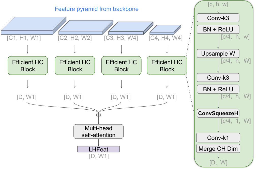
We propose an efficient height compression (EHC) module to extract the LHFeat $\mathbb{R}^{D\times W_{1}}$ from the backbone’s feature pyramid. We detail the EHC module in Sec. 3.2.

Predicting modalities.

We use $N$ in this work to denote the number of target channels for a task (e.g., $N$ is set to $1$ for depth estimation and is set to the number of classes for semantic segmentation). Given the LHFeat $\mathbb{R}^{D\times W_{1}}$ , we show how HoHoNet predicts 1D output $\mathbb{R}^{N\times W_{\mathrm{inp.}}}$ in Sec. 3.3. In Sec. 3.4, we propose the first method to yield 2D dense prediction $\mathbb{R}^{N\times H_{\mathrm{inp.}}\times W_{\mathrm{inp.}}}$ from the compact LHFeat, which widely extends the potential applications of the proposed efficient framework.

3.2 EHC module for LHFeat

The proposed efficient height compression (EHC) module is illustrated in Fig. 4. We first employ EHC blocks to squeeze the height of each 2D feature from the backbone’s pyramid. The resulting 1D features are then simply fused by summation. Within the EHC block, the input 2D features are first processed by a $\operatorname{Conv2D}$ block for channel reduction, and then the spatial width is upsampled to $W_{1}$ if needed, and finally, another $\operatorname{Conv2D}$ block refines the upsampled features. To efficiently reduce the feature height to $1$ , we design the $\operatorname{ConvSqueezeH}$ layer, a depthwise convolution layer with kernel size set to $(h,1)$ to cover full feature height without padding. Note that the parameter $h$ of each EHC block is automatically pre-computed given $H_{\mathrm{inp.}}$ . Finally, a $\operatorname{Conv2D}$ layer converts the number of channels to LHFeat’s latent size $D$ , and the height dimension is simply discarded as it is already reduced to $1$ by the $\operatorname{ConvSqueezeH}$ layer.

To further refine the initial LHFeat, the similar prior work SunHSC19 adopts bidirectional LSTM HochreiterS97 for horizontal prediction. We find the recurrent layer accounts for 22% of our deep net processing time, so we employ multi-head self-attention VaswaniSPUJGKP17 (MHSA) instead. Our results show that MHSA runs faster and improves accuracy more.

3.3 Predicting 1D per-column modalities

The target modality of some applications can be formulated into per-column prediction instead of the conventional per-pixel format. An example in this regard has been shown by Sun et al. SunHSC19 for layout estimation. To predict the 1D modalities, we first upsample the horizontal features from $\mathbb{R}^{D\times W_{1}}$ to $\mathbb{R}^{D\times W_{\mathrm{inp.}}}$ and apply three $\operatorname{Conv1D}$ layers of kernel size $3$ , $3$ , and $1$ respectively with $\operatorname{BN}$ , $\operatorname{ReLU}$ in between. The last layer yields the final prediction in $\mathbb{R}^{N\times W_{\mathrm{inp.}}}$ .

3.4 Predicting 2D per-pixel modalities

The strategy of shaping output space into per-column format does not apply to tasks that involve per-pixel modalities. Here we present the horizon-to-dense module of HoHoNet to derive dense prediction $\mathbb{R}^{N\times H_{\mathrm{inp.}}\times W_{\mathrm{inp.}}}$ from the compact LHFeat $\mathbb{R}^{D\times W_{1}}$ . This functionality opens the door to a more common scenario for various applications.

The trainable layers for 2D modality prediction are almost the same as the layers for 1D prediction introduced in Sec. 3.3 except that the number of channels in the output layer is augmented to $E=N\cdot r$ where $N$ is the number of target channels for a task and $r$ is the number of components shared by a image column. The produced prediction is then reshaped from $\mathbb{R}^{E\times W_{\mathrm{inp.}}}$ to $\mathbb{R}^{N\times r\times W_{\mathrm{inp.}}}$ . We present two different operations to recover $\mathbb{R}^{r}$ back to $\mathbb{R}^{H_{\mathrm{inp.}}}$ for each column depending on the physical meaning we assign to the $r$ predicted values.

Interpolation.

The simplest way is to view the latent dimension $r$ as the output height and apply linear interpolation to resize $r$ to $H_{\mathrm{inp.}}$ if $r<H_{\mathrm{inp.}}$ .

Inverse discrete cosine transform (IDCT).

Inspired by the application of the DCT in image compression for its energy compaction property, we view the $r$ predicted values as if they are in the DCT frequency domain with higher frequencies being truncated. In this case, we can apply IDCT to recover the low-pass signal back to the original signal. Let $x=[x_{n}]_{n=0}^{r-1}\in\mathbb{R}^{r}$ be the prediction; the final output $X=[X_{m}]_{m=0}^{H-1}\in\mathbb{R}^{H}$ can be recovered by

X_{m}=\frac{x_{0}}{2}+\sum_{n=1}^{r-1}x_{n}\cos\left[\frac{\pi}{H}n\left(m+\frac{1}{2}\right)\right].

(1)

A unified view.

We can put the two aforementioned operations into a unified view of matrix multiplication as $X=Mx$ where $x\in\mathbb{R}^{r}$ , $X\in\mathbb{R}^{H}$ , and $M\in\mathbb{R}^{H\times r}$ consisting of $r$ orthogonal column vectors. Depending on the choice of basis, this unified view can implement linear interpolation or IDCT, as shown in Fig. 5.

We find that IDCT constantly outperforms linear interpolation. We elaborate the intuition as follows. The LHFeat blends the spatial-row information (as described in Sec. 3.2), so training the last layers to disentangle the row-dependent dense modality from the flattened row-less LHFeat would pose a challenge. Conversely, learning to predict in the frequency domain can benefit from the well defined basis functions with meaningful spatial frequencies that characterize each column’s original row information as a whole, and therefore may alleviate the row-dependency problem.

4 Experiments

In Sec. 4.1, we first conduct ablation studies for the proposed components in HoHoNet. We then compare the performance of HoHoNet with state-of-the-art methods on dense depth estimation (Sec. 4.2), semantic segmentation (Sec. 4.3), and layout estimation (Sec. 4.4). Note that we train HoHoNet for each task separately and focus on showcasing the effectiveness of HoHoNet in learning a modality. In Sec. 4.5, we analyze the effect of non-gravity-aligned view. More quantitative and qualitative results are included in the supplementary material.

4.1 Ablation study

Table 1 summarizes the results of ablation experiments, where we compare different settings of HoHoNet for dense depth estimation. Detailed descriptions are as follows.

Ablation split for Matterport3D ChangDFHNSSZZ17.

Matterport3D is a large-scale real-world dataset of indoor panoramas. We prepare the ablation split by splitting the official 61 training houses into 41 and 20 houses (containing 4,921 and 2,908 panoramas) for training and validation during ablation study. We do not use the official validation split for ablation study as it will be used for state-of-the-art comparison later. The input ERPs are resized to $512\times 1024$ .

Training and evaluation.

We use Adam KingmaB14 to optimize the L1 loss for 40 epochs with batch-size of 4. The learning rate is set to 1e-4, and we apply polynomial learning rate decay with factor $0.9$ . Standard depth evaluation metric—MAE, RMSE, and $\delta^{1}$ —are used. We measure the average frame per second (FPS) for processing 50 individual $512\times 1024$ panoramas on a GeForce RTX 2080 Ti.

Architecture of LHFeat extraction.

Table 1(a) compares the proposed efficient height compression (EHC) module with the architecture used in the related work SunHSC19. In SunHSC19, a sequence of convolution layers gradually reduces the feature heights to form the initial LHFeat, which is then followed by a bidirectional LSTM (Bi-LSTM) for feature refinement. (Detailed architectures are in the supplementary material.) Table 1(a) shows that employing the proposed EHC module for initial LHFeat extraction achieves better speed and accuracy under different refinement configurations. We also find that using multi-head self-attention for feature refinement provides a better speed-accuracy tradeoff. Finally, our overall architecture for extracting the LHFeat is considerably better than SunHSC19’s—the depth MAE is improved from $0.3002$ to $0.2835$ with FPS from $38$ to $52$ . All experiments in Table 1(a) deploy ResNet-50 as backbone and use the IDCT with $r=64$ for dense prediction.

HC	Refine	MAE $\downarrow$	RMSE $\downarrow$	$\delta^{1}\uparrow$	FPS $\uparrow$
SunHSC19	-	0.3090	0.5238	0.8158	49
EHC	-	0.3022	0.5102	0.8204	54
SunHSC19	Bi-LSTM	0.3002	0.5147	0.8254	38
EHC	Bi-LSTM	0.2928	0.5036	0.8294	41
SunHSC19	MHSA	0.2915	0.5035	0.8331	47
EHC	MHSA	0.2835	0.4916	0.8389	52

(a) Comparison of the components for LHFeat extraction. The ‘HC’ column indicates the height compression block, which produces the initial LHFeat from the backbone features. We compare the results of ‘no feature refinement’, ‘refined by bidirectional LSTM’ HochreiterS97 (Bi-LSTM), and ‘refined by multi-head self-attention’ VaswaniSPUJGKP17 (MHSA). Refinement with MHSA achieves the most favorable results.

$r$	Basis	MAE $\downarrow$	RMSE $\downarrow$	$\delta^{1}\uparrow$	FPS $\uparrow$
32	Interp.	0.2886	0.5013	0.8356	52
32	IDCT	0.2847	0.4935	0.8369	52
64	Interp.	0.2880	0.4996	0.8351	52
64	IDCT	0.2835	0.4916	0.8389	52
128	Interp.	0.2926	0.5043	0.8308	52
128	IDCT	0.2850	0.4955	0.8405	52
256	Interp.	0.2937	0.5059	0.8260	52
256	IDCT	0.2903	0.5028	0.8334	52
512	Interp.	0.3045	0.5189	0.8227	52
512	IDCT	0.2913	0.5040	0.8341	52

(b) Comparison on the different settings of the proposed horizon-to-dense module. The parameter

r

denotes the number of components in a basis. We compare the two bases that implement the linear interpolation (Interp.) and the inverse discrete cosine transform (IDCT).

Backbone	MAE $\downarrow$	RMSE $\downarrow$	$\delta^{1}\uparrow$	FPS $\uparrow$
ResNet34	0.2854	0.4976	0.8397	110
ResNet50	0.2835	0.4916	0.8389	52

Table 1: Ablation study on depth modality using the ablation split of Matterport3D ChangDFHNSSZZ17. More details are in Sec. 4.1.

Hyperparameters of horizon-to-dense.

We compare the two operations—linear interpolation (spatial domain) and IDCT (frequency domain)—applied to dense prediction under different basis setups. As shown in Table 1(b), learning to predict in frequency domain (with IDCT) is consistently better than predicting in spatial domain (with linear interpolation) for dense depth estimation upon the compact LHFeat. Interestingly, the number of components $r$ is not monotonic to the resulting accuracy, and we find $r=64$ is the best setting for our model. As the compared operations introduce negligible computational cost, the FPSs are almost identical even if we increase $r$ . All experiments in Table 1(b) share the same deep net setting that consists of ResNet-50, the proposed EHC, and the MHSA.

Comparison of the backbones.

We compare the results of different backbones in Table 1(c), where we find that employing ResNet-34 can almost double the FPS with only a little drop in accuracy comparing to ResNet-50.

Dataset	Method	MRE	MAE	RMSE	RMSE (log)	$\delta^{1}$	$\delta^{2}$	$\delta^{3}$
Matterport3D	FCRN LainaRBTN16	0.2409	0.4008	0.6704	0.1244	0.7703	0.9174	0.9617
	OmniDepth (bn) ZioulisKZD18	0.2901	0.4838	0.7643	0.1450	0.6830	0.8794	0.9429
	Equi WangYSCT20	0.2074	0.3701	0.6536	0.1176	0.8302	0.9245	0.9577
	Cube WangYSCT20	0.2505	0.3929	0.6628	0.1281	0.7556	0.9135	0.9612
	BiFuse WangYSCT20	0.2048	0.3470	0.6259	0.1134	0.8452	0.9319	0.9632
	Ours	0.1488	0.2862	0.5138	0.0871	0.8786	0.9519	0.9771
Stanford2D3D	FCRN LainaRBTN16	0.1837	0.3428	0.5774	0.1100	0.7230	0.9207	0.9731
	OmniDepth (bn) ZioulisKZD18	0.1996	0.3743	0.6152	0.1212	0.6877	0.8891	0.9578
	Equi WangYSCT20	0.1428	0.2711	0.4637	0.0911	0.8261	0.9458	0.9800
	Cube WangYSCT20	0.1332	0.2588	0.4407	0.0844	0.8347	0.9523	0.9838
	BiFuse WangYSCT20	0.1209	0.2343	0.4142	0.0787	0.8660	0.9580	0.9860
	Ours	0.1014	0.2027	0.3834	0.0668	0.9054	0.9693	0.9886

Table 2: State-of-the-art comparison for depth estimation on real-world indoor 360 datasets—Matterport3D ChangDFHNSSZZ17 and Stanford2D3D ArmeniSZS17. The evaluation protocol follows WangYSCT20, where the depth is clipped to 10 meter without depth median alignment.

4.2 Depth estimation

4.2.1 State-of-the-art comparison using the protocol of Wang et al. WangYSCT20

Datasets and evaluation protocol.

We compare HoHoNet with state-of-the-art 360 depth estimation methods on real-world datasets following the testing protocol of WangYSCT20. Matterport3D ChangDFHNSSZZ17 has 10,800 panoramas, and its training split contains 61 houses, and the testing results are reported on the merged official validation and test split. Stanford2D3D ArmeniSZS17 contains 1,413 panoramas, and the fold-1 is used where the fifth area is for testing, and the other areas are for training. All the ERP images and depth maps are resized to $512\times 1024$ . Standard depth estimation evaluation metrics—MRE, MAE, RMSE, RMSE (log), and $\delta$ —are used. Depths are clipped to 10 meters without median alignment.

Implementation details.

We employ ResNet-50 as the backbone with the proposed EHC module for LHFeat extraction; the latent size $D$ of LHFeat is set to $256$ ; IDCT with $r=64$ components is applied to the model predictions. We use Adam KingmaB14 to optimize the L1 loss for $60$ epochs with a batch-size of $4$ . The learning rate is set to 1e-4, and we apply the polynomial learning rate decay with factor $0.9$ .

Results.

Table 2 shows the comparisons with prior arts. We demonstrate that the proposed HoHoNet outperforms the previous state-of-the-art, BiFuse WangYSCT20, by a large margin. Note also that BiFuse takes both ERP and cubemap as their model inputs and thus requires two backbone networks. HoHoNet has only one backbone and the compact LHFeat can achieve superior results, which shows the effectiveness of the proposed framework.

A qualitative comparison with BiFuse WangYSCT20 is provided in Fig. 6, where we download their code¹¹ 1 https://github.com/Yeh-yu-hsuan/BiFuse and the pre-trained weights for the comparison. We find that HoHoNet is good at capturing the overall structure of the scene. However, some drawbacks of HoHoNet are also observable through the visualization in Fig. 6.

4.2.2 State-of-the-art comparison using the protocol of Jin et al. JinXZZTXYG20

Dataset and evaluation protocol.

We also compare HoHoNet with another set of methods following the testing protocol of JinXZZTXYG20. A subset of the real-world Stanford2D3D ArmeniSZS17 dataset with extra layout annotation is used, where there are only $404$ and $113$ panoramas for training and testing. All the ERP images and depth maps are resized to $256\times 512$ . Standard evaluation metrics—RMSE, MRE, log10, and $\delta^{1}$ —for depth estimation are used. Neither depth clipping nor median alignment is applied during evaluation.

Implementation details.

The network and the training details are the same as in Sec. 4.2.1. However, we find the training strategy of JinXZZTXYG20 is very different from ours. For a fair comparison, we also report the results of training HoHoNet with the training protocol of JinXZZTXYG20—SGD optimizer with a batch-size of $8$ , learning rate of $0.01$ , and weight decay set to 5e-4.

Results.

The comparison on the Stanford2D3D subset is shown in Table 3(a). HoHoNet achieves the best accuracy under the same training protocol, and using Adam optimizer with our training setting can further improve the results. Note that GeoReg360 JinXZZTXYG20 employs a ResNet-50 and a ResNet-34, and the network is jointly trained with the additional layout and semantic annotation. Conversely, HoHoNet employs a single ResNet-50 and is only trained with depth modality, but still shows superior results, which further demonstrates the effectiveness of the proposed framework.

Method	RMSE	MRE	log10	$\delta^{1}$
FCRN LainaRBTN16	0.534	0.164	0.073	0.749
UResNet ZioulisKZD18	0.590	0.187	0.084	0.711
RectNet ZioulisKZD18	0.577	0.181	0.081	0.717
Sph. FCRN TatenoNT18	0.523	0.145	0.067	0.783
U-Net RonnebergerFB15	0.472	0.140	0.062	0.803
GeoReg360 JinXZZTXYG20†	0.421	0.118	0.053	0.851
Ours*	0.408	0.111	0.050	0.867
Ours	0.394	0.104	0.048	0.896
*Using JinXZZTXYG20 training protocol for a fair comparison.
†Using layout and semantic annotation.

(a) Quantitative comparison for dense depth on Stanford2D3D ArmeniSZS17 layout-available subset ZouCSH18. We strictly follow JinXZZTXYG20 evaluation protocol. See detail in Sec. 4.2.2.

$H\times W$	Input	Method	mIoU	mAcc
Simple backbone w/ low-resolution $360\degree$
$64\times 128$	RGB-D	Gauge Net CohenWKW19	39.4	55.9
	RGB-D	UGSCNN JiangHKPMN19	38.3	54.7
	RGB-D	HexRUNet ZhangLSC19	43.3	58.6
	RGB-D	TangentImg EderSLF20	37.5	50.2
	RGB-D	Ours	40.8	52.1
$256\times 512$	RGB-D	TangentImg EderSLF20	41.8	54.9
$256\times 512$	RGB-D	Ours	43.3	53.9
ResNet backbone w/ high-resolution $360\degree$
$2048\times 4096$	RGB	TangentImg EderSLF20	45.6	65.2
$1024\times 2048$	RGB	Ours	52.0	65.0
$2048\times 4096$	RGB-D	TangentImg EderSLF20	51.9	69.1
$1024\times 2048$	RGB-D	Ours	56.3	68.9

(b) Quantitative comparison for semantic segmentation on Stanford2D3D ArmeniSZS17. Results are averaged over the official 3 folds.

Method	Backbone	IoU		FPS
Method	Backbone	3D	2D	FPS
LayoutNet v2 ZouSPCSWCH19	ResNet-34	75.82	78.73	46
DuLa-Net v2 YangWPWSC19	ResNet-50	75.05	78.82	34
HorizonNet SunHSC19	ResNet-50	79.11	81.71	31
AtlantaNet PintoreAG20	ResNet-50	80.02	82.09	5
Ours	ResNet-34	79.88	82.32	110

Table 3: State-of-the-art comparison on various datasets and different modalities.

4.3 Semantic segmentation

Dataset and evaluation protocol.

We evaluate HoHoNet’s semantic segmentation performance on Stanford2D3D ArmeniSZS17 dataset. As previous work, we report the averaged results from the official 3-fold cross-validation splits, using standard semantic segmentation evaluation metrics—class-wise mIoU and class-wise mAcc.

Implementation detail.

The architecture setting of HoHoNet for semantic segmentation is almost the same as for depth estimation in Sec. 4.2.1 except the last layer has $E=Nr=13\cdot 64=832$ channels. To compare with methods using a simple backbone under low resolution, we follow EderSLF20; JiangHKPMN19; ZhangLSC19 to construct a shallow U-Net but purely with planar CNN. For results on high resolution, we use ResNet-101 as backbone. We use Adam KingmaB14 to optimize the cross-entropy loss for $60$ epochs with a batch-size of $4$ . The learning rate is 1e-4 with polynomial decay of factor $0.9$ .

Results.

Table 3(b) shows the comparison with previous methods. On the lowest resolution, HexRUNet ZhangLSC19, with a specially designed kernel on icosahedron representation, achieves the best result. Ours with purely planar CNNs and compact LHFeat is still competitive with the distortion mitigated methods under the low-resolution settings. When scaling to a high resolution, we achieve similar mACC with the recent state-of-the-art EderSLF20, while our mIoU is significantly better. Note that the results of EderSLF20 are obtained from a stronger FCN-ResNet101 backbone and a higher input resolution. Limited by our device and ERP projection, we can only train on a lower $1024\times 2048$ resolution but still obtain competitive performance with the current state-of-the-art on $360\degree$ semantic segmentation.

4.4 Room layout estimation

Dataset and evaluation protocol.

We use MatterportLayout ZouSPCSWCH19; WangYSCT20Layout dataset, which is a real-world 360 Manhattan layout dataset. The official evaluation function²² 2 https://github.com/zouchuhang/LayoutNetv2 for 2D IoU and 3D IoU is used directly, where the 2D IoU is measured by projecting floor corners to an aligned floor, while 3D IoU is for pop-up view considering both floor and ceiling corners.

Implementation details.

HoHoNet is compatible with the 1D layout representation proposed by HorizonNet SunHSC19. Since our main focus is not to design a new method for layout reconstruction, we use SunHSC19’s loss, training protocol, and post-processing algorithm directly. We find HoHoNet with ResNet-34 shows slightly better accuracy than ResNet-50 in validation, so we use the simpler ResNet-34 as backbone.

Results.

The comparison with previous methods on MatterportLayout is shown in Table 3(c). The FPSs are obtained using the official codes2³³ 3 https://github.com/SunDaDenny/DuLa-Net⁴⁴ 4 https://github.com/sunset1995/HorizonNet⁵⁵ 5 https://github.com/crs4/AtlantaNet and measured by the averaged feed-forward times of the models on a GeForce RTX 2080 Ti. The result of AtlantaNet PintoreAG20 is obtained from their official new pre-trained weights5 with aligned data split and re-evaluated by the official evaluation function2. Our result is on par with the state-of-the-art AtlantaNet but $22\times$ faster. HoHoNet also outperforms HorizonNet SunHSC19 by $+0.77$ 3D IoU and $+0.61$ 2D IoU, and is $3.5\times$ faster, which shows the effectiveness of the designed architecture.

4.5 Results on non-gravity-aligned views

In Fig. 2, we show that the structure signals of an image column suffer more losses in compression if the image’s $y$ -axis is not aligned with the gravity. Though the 360 data in all benchmarks we use are mostly well-aligned with gravity, the captured $360\degree$ views could be non-gravity-aligned in practice. In Table 4, we show the vulnerability of our model to heavy pitch or roll rotation (see Fig. 2(c) and Fig. 2(b) for visualization). The pre-trained model in our ablation study takes the rotated images directly as input, and the output depth maps are rotated back to the original view for a fair comparison. As expected, the pre-trained model performs poorly when input $360\degree$ views are not gravity-aligned. Introducing $10\degree$ of pitch or roll rotation increases MAE from $28.45$ cm to more than $44$ cm. A simple solution is to use the IMU sensor or 360 vanishing point detection algorithm ZhangSTX14; ZouCSH18 to ensure gravity alignment (the VP alignment is also a standard step in 360 layout benchmark WangYSCT20Layout; ZouCSH18; ZouSPCSWCH19).

We also show the results by training with $\mathcal{U}(-30\degree,30\degree)$ pitch/roll rotation as data augmentation, which makes the model much more robust against the non-canonical view but sacrifices the test-time performance when input $360\degree$ view are gravity-aligned (MAE $\uparrow$ from $28.35$ cm to $30.92$ cm).

Training Rot. Aug.	Testing Cam. Rot.	MAE (cm)
Training Rot. Aug.	Testing Cam. Rot.	$0\degree$	$10\degree$	$20\degree$	$30\degree$
	Pitch	28.35	44.88	62.77	75.79
✓	Pitch	30.92	31.30	31.80	32.97
	Roll	28.35	44.32	61.90	75.11
✓	Roll	30.92	31.32	31.80	32.90

Table 4: Vulnerability to non-gravity-aligned views.

5 Conclusion

This work presents a novel framework, HoHoNet, which is the first step to learning compact latent horizontal features for dense modalities modeling of omnidirectional images. HoHoNet is fast, versatile, and accurate for solving layout reconstruction, depth estimation, and semantic segmentation with accuracy on par with or better than the state-of-the-art.

Acknowledgements:

This work was supported in part by the MOST, Taiwan under Grants 110-2634-F-001-009 and 110-2634-F-007-016, MOST Joint Research Center for AI Technology and All Vista Healthcare. We thank National Center for High-performance Computing (NCHC) for providing computational and storage resources.

Supplementary material

A Network architecture diagram

We show the detailed architecture diagram in Fig. 7. The shape of each feature tensor is denoted as “# of channels, height, width” within the box. The height and width of the input panorama are assumed to be $512$ and $1024$ respectively. $D$ and $E$ are hyperparameters. The $\operatorname{ConvSqueezeH}$ layer is a depthwise convolution layer with kernel size set to the prior known input feature height without padding, which produces output feature height $1$ .

Figure 7: The detailed network architecture with ResNet50 HeZRS16 backbone.

B Comparing EHC block and HC block SunHSC19

The height compression block aims to squeeze a 2D feature from the backbone to produce a 1D horizontal feature. Fig. 8 shows the architecture of our Efficient Height Compression block (EHC block) and the one of HC block SunHSC19 for comparison. The HC block SunHSC19 employs a sequence of convolution layers to gradually reduce the number of channels and heights, while we first use a convolution layer for channel reduction and then use bilinear upsampling and $\operatorname{ConvSqueezeH}$ layer to produce the features in horizontal shape. We show in our ablation experiments that replacing the HC block SunHSC19 with the proposed ECH block leads to better speed and accuracy.

C Detailed semantic segmentation results

We show detailed per-class IoU and per-class Acc for semantic segmentation in Table 5. We achieve the best IoU on 10 out of 13 classes and superior overall mIoU; we achieve best Acc on 7 out of 13 classes and comparable overall mAcc.

Method	overall	beam	board	bookcase	ceiling	chair	clutter	column	door	floor	sofa	table	wall	window
Low-resolution RGB-D
UGSCNN JiangHKPMN19	38.3	8.7	32.7	33.4	82.2	42.0	25.6	10.1	41.6	87.0	7.6	41.7	61.7	23.5
HexRUNet ZhangLSC19	43.3	10.9	39.7	37.2	84.8	50.5	29.2	11.5	45.3	92.9	19.1	49.1	63.8	29.4
TangentImg EderSLF20	37.5	10.9	26.6	31.9	82.0	38.5	29.3	5.9	36.2	89.4	12.6	40.4	56.5	26.7
Ours	40.8	3.6	43.5	40.6	81.8	41.3	27.7	9.2	52.0	92.2	9.4	44.6	61.6	23.4
High-resolution RGB-D
TangentImg EderSLF20	51.9	4.5	49.9	50.3	85.5	71.5	42.4	11.7	50.0	94.3	32.1	61.4	70.5	50.0
Ours	56.3	7.4	62.3	55.5	87.0	66.4	44.3	19.2	66.5	96.1	43.3	60.1	72.9	51.4

(a) Per-class IoU (%).

Method	overall	beam	board	bookcase	ceiling	chair	clutter	column	door	floor	sofa	table	wall	window
Low-resolution RGB-D
UGSCNN JiangHKPMN19	54.7	19.6	48.6	49.6	93.6	63.8	43.1	28.0	63.2	96.4	21.0	70.0	74.6	39.0
HexRUNet ZhangLSC19	58.6	23.2	56.5	62.1	94.6	66.7	41.5	18.3	64.5	96.2	41.1	79.7	77.2	41.1
TangentImg EderSLF20	50.2	25.6	33.6	44.3	87.6	51.5	44.6	12.1	64.6	93.6	26.2	47.2	78.7	42.7
Ours	52.1	9.5	56.5	56.6	95.1	57.9	40.7	12.5	64.5	96.8	10.6	69.1	79.3	28.4
High-resolution RGB-D
TangentImg EderSLF20	69.1	22.6	62.0	70.0	90.3	84.7	55.5	41.4	76.7	96.9	70.3	73.9	80.1	74.3
Ours	68.9	16.7	79.0	71.8	96.4	79.2	59.7	26.9	77.7	98.2	58.0	79.6	85.9	66.3

(b) Per-class Acc (%).

Table 5: Detailed quantitative per-class results on Stanford2D3D ArmeniSZS17 with RGB-D as input.

D Detailed layout estimation results

We show detailed quantitative results for room layout under different numbers of ground truth 2D corners in Table 6. Our training protocol and layout formalization are identical to HorizonNet SunHSC19, while we observe improvements (except rooms with six corners) by using our network architecture. In comparison with the most recent state-of-the-art—AtlantaNet PintoreAG20, we show better results on scenes with fewer corners and similar accuracy on overall scenes; meanwhile, our model is $22\times$ faster than AtlantaNet PintoreAG20.

Method	Metric	# of corners
Method	Metric	overall	4	6	8	10+
LayoutNet v2 ZouSPCSWCH19	3D IoU (%)	75.82	81.35	72.33	67.45	63.00
DuLa-Net v2 YangWPWSC19		75.07	77.02	78.79	71.03	63.27
HorizonNet SunHSC19		79.11	81.88	82.26	71.78	68.32
AtlantaNet PintoreAG20		80.02	82.09	82.08	75.19	71.61
Ours		79.88	82.64	82.16	73.65	69.26
LayoutNet v2 ZouSPCSWCH19	2D IoU (%)	78.73	84.61	75.02	69.79	65.14
DuLa-Net v2 YangWPWSC19		78.82	81.12	82.69	74.00	66.12
HorizonNet SunHSC19		81.71	84.67	84.82	73.91	70.58
AtlantaNet PintoreAG20		82.09	84.42	83.85	76.97	73.18
Ours		82.32	85.26	84.81	75.59	70.98

Table 6: Detailed quantitative comparison for room layout estimation on MatterportLayout ZouSPCSWCH19 under different numbers of ground-truth corners.

E More qualitative comparisons for depth estimation

We show more qualitative comparisons with the prior art—BiFuse WangYSCT20—in Fig. 9. BiFuse’s results are obtained from their official released model trained on the real-world Matterport3D ChangDFHNSSZZ17 dataset.

F Qualitative results for semantic segmentation

Qualitative results for semantic segmentation on Stanford2D3D ArmeniSZS17 dataset are shown in Fig. 10. We fail to build the prior art EderSLF20 from their public release for semantic segmentation on high-resolution panorama, so we only show our results.

G Qualitative comparisons for layout estimation

We show qualitative comparisons for room layout estimation with the prior art—AtlantaNet PintoreAG20—in Fig. 11. The results of AtlantaNet are obtained from their official code and pre-trained weights. We use SunHSC19 post-processing algorithm to produce Manhattan layouts; AtlantaNet PintoreAG20’s algorithm generates less restrictive Atlanta layouts. Our model achieves promising results comparable to the most recent AtlantaNet PintoreAG20, while our model runs $22\times$ faster.

References

(1) Iro Armeni, Sasha Sax, Amir Roshan Zamir, and Silvio Savarese. Joint 2d-3d-semantic data for indoor scene understanding. CoRR, abs/1702.01105, 2017.
(2) Angel X. Chang, Angela Dai, Thomas A. Funkhouser, Maciej Halber, Matthias Nießner, Manolis Savva, Shuran Song, Andy Zeng, and Yinda Zhang. Matterport3d: Learning from RGB-D data in indoor environments. In 2017 International Conference on 3D Vision, 3DV 2017, Qingdao, China, October 10-12, 2017, pages 667–676. IEEE Computer Society, 2017.
(3) Devendra Singh Chaplot, Ruslan Salakhutdinov, Abhinav Gupta, and Saurabh Gupta. Neural topological SLAM for visual navigation. In 2020 IEEE/CVF Conference on Computer Vision and Pattern Recognition, CVPR 2020, Seattle, WA, USA, June 13-19, 2020, pages 12872–12881. IEEE, 2020.
(4) Hsien-Tzu Cheng, Chun-Hung Chao, Jin-Dong Dong, Hao-Kai Wen, Tyng-Luh Liu, and Min Sun. Cube padding for weakly-supervised saliency prediction in 360° videos. In 2018 IEEE Conference on Computer Vision and Pattern Recognition, CVPR 2018, Salt Lake City, UT, USA, June 18-22, 2018, pages 1420–1429. IEEE Computer Society, 2018.
(5) Taco Cohen, Maurice Weiler, Berkay Kicanaoglu, and Max Welling. Gauge equivariant convolutional networks and the icosahedral CNN. In Kamalika Chaudhuri and Ruslan Salakhutdinov, editors, Proceedings of the 36th International Conference on Machine Learning, ICML 2019, 9-15 June 2019, Long Beach, California, USA, volume 97 of Proceedings of Machine Learning Research, pages 1321–1330. PMLR, 2019.
(6) Taco S. Cohen, Mario Geiger, Jonas Köhler, and Max Welling. Spherical cnns. In 6th International Conference on Learning Representations, ICLR 2018, Vancouver, BC, Canada, April 30 - May 3, 2018, Conference Track Proceedings. OpenReview.net, 2018.
(7) Benjamin Coors, Alexandru Paul Condurache, and Andreas Geiger. Spherenet: Learning spherical representations for detection and classification in omnidirectional images. In Vittorio Ferrari, Martial Hebert, Cristian Sminchisescu, and Yair Weiss, editors, Computer Vision - ECCV 2018 - 15th European Conference, Munich, Germany, September 8-14, 2018, Proceedings, Part IX, volume 11213 of Lecture Notes in Computer Science, pages 525–541. Springer, 2018.
(8) Marc Eder, Pierre Moulon, and Li Guan. Pano popups: Indoor 3d reconstruction with a plane-aware network. In 2019 International Conference on 3D Vision, 3DV 2019, Québec City, QC, Canada, September 16-19, 2019, pages 76–84. IEEE, 2019.
(9) Marc Eder, Mykhailo Shvets, John Lim, and Jan-Michael Frahm. Tangent images for mitigating spherical distortion. In 2020 IEEE/CVF Conference on Computer Vision and Pattern Recognition, CVPR 2020, Seattle, WA, USA, June 13-19, 2020, pages 12423–12431. IEEE, 2020.
(10) Kaiming He, Xiangyu Zhang, Shaoqing Ren, and Jian Sun. Deep residual learning for image recognition. In 2016 IEEE Conference on Computer Vision and Pattern Recognition, CVPR 2016, Las Vegas, NV, USA, June 27-30, 2016, pages 770–778. IEEE Computer Society, 2016.
(11) Sepp Hochreiter and Jürgen Schmidhuber. Long short-term memory. Neural Comput., 9(8):1735–1780, 1997.
(12) Chiyu Max Jiang, Jingwei Huang, Karthik Kashinath, Prabhat, Philip Marcus, and Matthias Nießner. Spherical cnns on unstructured grids. In 7th International Conference on Learning Representations, ICLR 2019, New Orleans, LA, USA, May 6-9, 2019. OpenReview.net, 2019.
(13) Lei Jin, Yanyu Xu, Jia Zheng, Junfei Zhang, Rui Tang, Shugong Xu, Jingyi Yu, and Shenghua Gao. Geometric structure based and regularized depth estimation from 360 indoor imagery. In 2020 IEEE/CVF Conference on Computer Vision and Pattern Recognition, CVPR 2020, Seattle, WA, USA, June 13-19, 2020, pages 886–895. IEEE, 2020.
(14) Diederik P. Kingma and Jimmy Ba. Adam: A method for stochastic optimization. In Yoshua Bengio and Yann LeCun, editors, 3rd International Conference on Learning Representations, ICLR 2015, San Diego, CA, USA, May 7-9, 2015, Conference Track Proceedings, 2015.
(15) Iro Laina, Christian Rupprecht, Vasileios Belagiannis, Federico Tombari, and Nassir Navab. Deeper depth prediction with fully convolutional residual networks. In Fourth International Conference on 3D Vision, 3DV 2016, Stanford, CA, USA, October 25-28, 2016, pages 239–248. IEEE Computer Society, 2016.
(16) Yeon Kun Lee, Jaeseok Jeong, Jong Seob Yun, Wonjune Cho, and Kuk-Jin Yoon. Spherephd: Applying cnns on a spherical polyhedron representation of 360deg images. In IEEE Conference on Computer Vision and Pattern Recognition, CVPR 2019, Long Beach, CA, USA, June 16-20, 2019, pages 9181–9189. Computer Vision Foundation / IEEE, 2019.
(17) Giovanni Pintore, Marco Agus, and Enrico Gobbetti. Atlantanet: Inferring the 3D indoor layout from a single 360 image beyond the manhattan world assumption. In Proceedings of The European Conference on Computer Vision (ECCV), 2020.
(18) Olaf Ronneberger, Philipp Fischer, and Thomas Brox. U-net: Convolutional networks for biomedical image segmentation. In Nassir Navab, Joachim Hornegger, William M. Wells III, and Alejandro F. Frangi, editors, Medical Image Computing and Computer-Assisted Intervention - MICCAI 2015 - 18th International Conference Munich, Germany, October 5 - 9, 2015, Proceedings, Part III, volume 9351 of Lecture Notes in Computer Science, pages 234–241. Springer, 2015.
(19) Yu-Chuan Su and Kristen Grauman. Learning spherical convolution for fast features from 360° imagery. In Isabelle Guyon, Ulrike von Luxburg, Samy Bengio, Hanna M. Wallach, Rob Fergus, S. V. N. Vishwanathan, and Roman Garnett, editors, Advances in Neural Information Processing Systems 30: Annual Conference on Neural Information Processing Systems 2017, 4-9 December 2017, Long Beach, CA, USA, pages 529–539, 2017.
(20) Yu-Chuan Su and Kristen Grauman. Kernel transformer networks for compact spherical convolution. In IEEE Conference on Computer Vision and Pattern Recognition, CVPR 2019, Long Beach, CA, USA, June 16-20, 2019, pages 9442–9451. Computer Vision Foundation / IEEE, 2019.
(21) Cheng Sun, Chi-Wei Hsiao, Min Sun, and Hwann-Tzong Chen. HorizonNet: learning room layout with 1d representation and pano stretch data augmentation. In IEEE Conference on Computer Vision and Pattern Recognition, CVPR 2019, Long Beach, CA, USA, June 16-20, 2019, pages 1047–1056, 2019.
(22) Keisuke Tateno, Nassir Navab, and Federico Tombari. Distortion-aware convolutional filters for dense prediction in panoramic images. In Vittorio Ferrari, Martial Hebert, Cristian Sminchisescu, and Yair Weiss, editors, Computer Vision - ECCV 2018 - 15th European Conference, Munich, Germany, September 8-14, 2018, Proceedings, Part XVI, volume 11220 of Lecture Notes in Computer Science, pages 732–750. Springer, 2018.
(23) Ashish Vaswani, Noam Shazeer, Niki Parmar, Jakob Uszkoreit, Llion Jones, Aidan N. Gomez, Lukasz Kaiser, and Illia Polosukhin. Attention is all you need. In Isabelle Guyon, Ulrike von Luxburg, Samy Bengio, Hanna M. Wallach, Rob Fergus, S. V. N. Vishwanathan, and Roman Garnett, editors, Advances in Neural Information Processing Systems 30: Annual Conference on Neural Information Processing Systems 2017, 4-9 December 2017, Long Beach, CA, USA, pages 5998–6008, 2017.
(24) Fu-En Wang, Yu-Hsuan Yeh, Min Sun, Wei-Chen Chiu, and Yi-Hsuan Tsai. Bifuse: Monocular 360 depth estimation via bi-projection fusion. In 2020 IEEE/CVF Conference on Computer Vision and Pattern Recognition, CVPR 2020, Seattle, WA, USA, June 13-19, 2020, pages 459–468. IEEE, 2020.
(25) Fu-En Wang, Yu-Hsuan Yeh, Min Sun, Wei-Chen Chiu, and Yi-Hsuan Tsai. Layoutmp3d: Layout annotation of matterport3d. CoRR, abs/2003.13516, 2020.
(26) Shang-Ta Yang, Fu-En Wang, Chi-Han Peng, Peter Wonka, Min Sun, and Hung-Kuo Chu. Dula-net: A dual-projection network for estimating room layouts from a single RGB panorama. In IEEE Conference on Computer Vision and Pattern Recognition, CVPR 2019, Long Beach, CA, USA, June 16-20, 2019, pages 3363–3372. Computer Vision Foundation / IEEE, 2019.
(27) Wei Zeng, Sezer Karaoglu, and Theo Gevers. Joint 3d layout and depth prediction from a single indoor panorama image. In Andrea Vedaldi, Horst Bischof, Thomas Brox, and Jan-Michael Frahm, editors, Computer Vision - ECCV 2020 - 16th European Conference, Glasgow, UK, August 23-28, 2020, Proceedings, Part XVI, volume 12361 of Lecture Notes in Computer Science, pages 666–682. Springer, 2020.
(28) Chao Zhang, Stephan Liwicki, William Smith, and Roberto Cipolla. Orientation-aware semantic segmentation on icosahedron spheres. In 2019 IEEE/CVF International Conference on Computer Vision, ICCV 2019, Seoul, Korea (South), October 27 - November 2, 2019, pages 3532–3540. IEEE, 2019.
(29) Yinda Zhang, Shuran Song, Ping Tan, and Jianxiong Xiao. Panocontext: A whole-room 3d context model for panoramic scene understanding. In David J. Fleet, Tomás Pajdla, Bernt Schiele, and Tinne Tuytelaars, editors, Computer Vision - ECCV 2014 - 13th European Conference, Zurich, Switzerland, September 6-12, 2014, Proceedings, Part VI, volume 8694 of Lecture Notes in Computer Science, pages 668–686. Springer, 2014.
(30) Jia Zheng, Junfei Zhang, Jing Li, Rui Tang, Shenghua Gao, and Zihan Zhou. Structured3d: A large photo-realistic dataset for structured 3d modeling. In Proceedings of The European Conference on Computer Vision (ECCV), 2020.
(31) Nikolaos Zioulis, Antonis Karakottas, Dimitrios Zarpalas, and Petros Daras. Omnidepth: Dense depth estimation for indoors spherical panoramas. In Vittorio Ferrari, Martial Hebert, Cristian Sminchisescu, and Yair Weiss, editors, Computer Vision - ECCV 2018 - 15th European Conference, Munich, Germany, September 8-14, 2018, Proceedings, Part VI, volume 11210 of Lecture Notes in Computer Science, pages 453–471. Springer, 2018.
(32) Chuhang Zou, Alex Colburn, Qi Shan, and Derek Hoiem. Layoutnet: Reconstructing the 3d room layout from a single RGB image. In 2018 IEEE Conference on Computer Vision and Pattern Recognition, CVPR 2018, Salt Lake City, UT, USA, June 18-22, 2018, pages 2051–2059. IEEE Computer Society, 2018.
(33) Chuhang Zou, Jheng-Wei Su, Chi-Han Peng, Alex Colburn, Qi Shan, Peter Wonka, Hung-Kuo Chu, and Derek Hoiem. 3d manhattan room layout reconstruction from a single 360 image. CoRR, abs/1910.04099, 2019.