Optimal Power Control for DoS Attack over Fading Channel: A Game-Theoretic Approach

In a typical wireless communication channel the transmitted signal suffers attenuation and distortion resulted from interference, shadowing, process noise, and fading, and all these factors can frequently result in packet dropout [25].

The wireless communication network is generally time-varying. In an industrial setting this time-variant characteristic may be resulted from moving machines, buildings, obstacle, and so forth, the receptor or the sender built on a moving device can also result in the time-variable property of the channel. Hence, except for the propagation path loss, channels also suffer shadowing and small-scale fading.

The architecture of wireless communication channel is depicted in Fig. 2. All frequency elements of the communication packet suffer a analogical fading or damping. As a result, the obtained signal at the receptor is provided as

where $s_{t}$ denotes the channel input which has an average energy constraint $E[s^{2}_{t}]\leq P$. $r_{t}$ represents the channel output; ${\varpi_{t}}$ is an additive white Gaussian noise (AWGN) whose mean is zero and variance is $\sigma_{\varpi}^{2}$. Throughout the article, we will refer to the attenuation ${g_{t}}$ simply as the fading channel gain.

Considering that the main characteristics of fading channels is a correlated, time-varying stochastic process. Specifically, the wireless transmission channel is a dynamic system, and the fading channel gain ${g_{t}}$ is a random process that transforms over time. An easy-to-handle mathematical model is needed to precisely describe the dynamic characteristics of time-varying fading channel. In this paper, the common scheme such as finite state Markov chain (FSMC) is utilized to model wireless fading channels. It is assumed throughout the paper that the following assumption holds:

Finite state channel models (FSCM) have been widely accepted as an effective method to describe the related structure of the fading channel [22]. The FSCM is characterized by a deterministic or probabilistic function of a first-order Markov chain, where each element may be related to a particular channel state. The Markov state process is in general stationary, therefore, the state transition probability is time-independent. And the distribution of initial state is assumed to be $u=[\mu_{1},\mu_{2},...,\mu_{l}]$. This is a common assumption in a real communication scenario for channel statistics are not fast-changing over time [22].

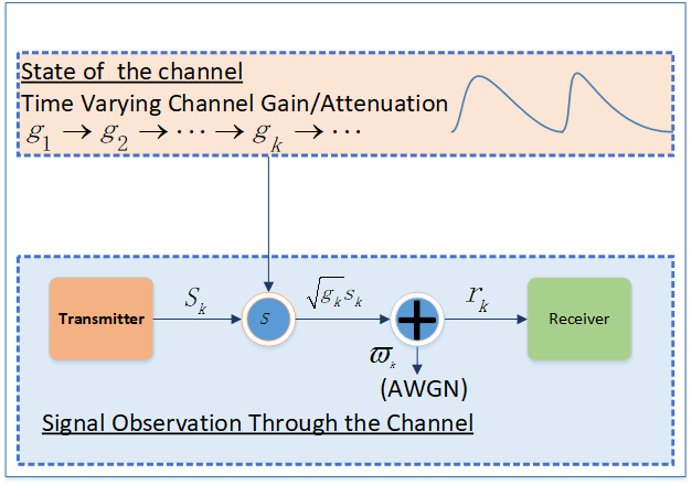
Random data packet dropout will take place due to fading and interference. To describe this scenario, we adopt an Additive White Gaussian Noise (AWGN) network, which chooses Quadrature Amplitude Modulation (QAM), to describe the communication between the transmitter and the receiver. After that, the symbol error rate (SER) is tightly connected with the signal to noise ratio (SNR) as $SER=2Q(\sqrt{\alpha SNR}),$ where $\alpha>0$ is a parameter and $Q(x)\triangleq\frac{1}{\sqrt{2\pi}}\int_{x}^{\infty}exp(-\eta^{2}/2)d\eta$. Consider a DoS attack congests the communication channel of the network. The corresponding SNR of the channel is transformed to SINR:

where $\Psi^{s}$ is the transmitted energy used by the sensor, $g^{s}$ represents the channel gain for sensors, $\Psi^{a}$ is the interfering energy from the attacker, $g^{a}$ represents the channel gain for attackers, and $\sigma^{2}$ represents the additive white Gaussian noise. Thus taking account of both fading and additive white Gaussian noise in the transmission, whether the signals transmitted by the sensor are successfully accepted by the remote center can be formulated as a binary random process ${\gamma_{k}},k\in\mathbb{N}$ (which indeed follows a Bernoulli distribution), in which $\gamma_{k}=0$ indicates that the packet has been lost.

Denote the energy levels of the sensor and the attacker, respectively, as:

The successful packet reception is not only statistically determined by the power levels but also by the channel gains of the sensor and the attacker.

This finite state fading channel model generates an error symbol based on the following probabilistic mechanism. At time $k$, the chain state of two player is $g^{s}_{k}$, $g^{a}_{k}$, respectively. It generates an output symbol $\gamma_{k}\in\{0,1\}$ with probability

where $\mathcal{P}_{s_{k}}\in\mathbb{P}_{\mathcal{S}}$, $\mathcal{P}_{a_{k}}\in\mathbb{P}_{\mathcal{A}}$, $g^{s}_{k}\in\Xi$ and $g^{a}_{k}\in\Xi$. Based on the state process and channel gains, the error symbol is memoryless, this is

To avoid trivial problems, we assume that the following equation holds: $\min_{\mathcal{P}_{s_{k}},g^{s}_{k},\mathcal{P}_{a_{k}},g^{a}_{k}}q(\mathcal{P}_{s_{k}},g^{s}_{k},\mathcal{P}_{a_{k}},g^{a}_{k})>1-\frac{1}{\rho(A)^{2}},$ where $A$ is the system matrix and $\rho(A)$ represents the spectral radius of $A$. Under the above sufficient condition, the expected estimation error covariance is bounded. While the above condition is not satisfied, the attacker would jam the channel with a certain interfering energy continuously to obtain an unbounded estimation error, that is to say, the attacker dominates the estimation process and thereby there exists no equilibrium for the attacker and sensor.

Denote $\hat{x}_{k}$ and $P_{k}$ as state estimate and corresponding error covariance of the system in the remote center side. According to the work [24], they can be obtained via the following procedure:

And $P_{k}$ is computed as follows:

where $\bar{P}$ represents the steady-state error covariance. Without loss of generality, we assume that the initial packet $\hat{x}^{s}_{0}$ is acquired by the remote center and hence $P_{0}=\bar{P}$.

In order to express succinctly, we define a random variable $\tau_{k}\in\mathbb{N}$ as the duration between two transmission:

which represents the distances between the time $k$ and the most recent time that the transmitted signal is acquired by the remote center. The estimation error covariance is associated with the holding time and the relationship is described as $P_{k}=h^{\tau_{k}}(\bar{P}),$ and the holding time updates as follows:

Note that the energy and channel gains of the two agents (the sensor and the attacker), i.e., $\mathcal{P}_{s_{k}},\mathcal{P}_{a_{k}},g^{s}_{k},g^{a}_{k}$ are given, and the sequence of stochastic variable $\tau_{k}$ forms a Markov chain with the transition probability matrix $\mathbb{T}$ given as follows:

where the elements of $\mathbb{T}$ represent the transition probability from the state $\tau_{k}=i$ to $\tau_{k+1}=j$, and the missing elements are $0$. And the probability $q=q(\mathcal{P}_{s_{k}},g^{s}_{k},\mathcal{P}_{a_{k}},g^{a}_{k})$ is given by (6). In the following subsection, we formulate the problem of interest.

Depending on the channel knowledge of sensors and attackers, we investigate how to adopt game theory to develop a transmission schedule for sensors and attackers under Nash equilibrium, where the choice of each player is the best response to the choice of other opponents. The sensor and the attacker are assumed to be rational and they will always adopt the behavior that offers the highest expected reward. Therefore, in this work, our goal is to find the optimal strategy for both sides such that no one obtains more through unilateral deviation. The complete information for the stochastic game is constructed as follows.

In this subsection, we first model the schedule of scheduling energy-efficient actions in an infinite time horizon. In other words, we investigate how to arrange the jamming power (or transmission energy) for the attacker (or the sensor) in a stochastic game framework. In this stochastic game framework, players decide action simultaneously. We assume that the state set and action set are discrete. The formal definition of this stochastic game is provided in the following:

In our problem, we provide the following specific content to describe the sensor-attacker game.

Player: We assume that the attacker and the sensor are all rational players. Denote by $\mathcal{I}^{1}$ the attacker and $\mathcal{I}^{2}$ the sensor. The attacker and the sensor decide the best action among all available choice for them in terms of their own goals.

State: The state space $\mathcal{S}$ can be expressed as $\mathcal{S}=\{(\tau_{k},g_{s},g_{a})\}$, where $\tau_{k}\in\mathbb{N}$, $g_{s}$ and $g_{a}$ are the channel gain of sensor and attacker, respectively. Notice that the holding time is tightly associated with the estimation error covariance $P_{k}$ as $P_{k}=h^{\tau_{k}}(\bar{P})$.

Action: Denote by $\mathcal{A}^{i}$ the action (or pure strategy) space for player $i$, $i=1,2$. At time $k$, the attacker decides the interfering energy $a_{k}\in\mathbb{P}_{\mathcal{A}}\triangleq[\mathcal{P}_{a_{1}},\cdots,\mathcal{P}_{a_{max}}]$, and the sensor selects the transmission energy $b_{k}\in\mathbb{P}_{\mathcal{S}}\triangleq[\mathcal{P}_{s_{1}},\cdots,\mathcal{P}_{s_{max}}].$ Denote by $(a_{k},b_{k})$ the joint action (or pure strategy) at time $k$.

Transition probability: Note that the holding time $\tau_{k}$ forms a Markov chain in which the transition matrix is presented in (14). And the transition probability is determined by the packet arrival probability in (6). From (15), $s_{k}$ has the Markov property. Denoted by $s_{k+1}=(\tau_{k+1},g_{s},g_{a}),s_{k}=(\tau_{k},g^{\prime}_{s},g^{\prime}_{a})\in\mathcal{S}$ and $a\in\mathbb{P}_{\mathcal{A}},b\in\mathbb{P}_{\mathcal{S}}$, $g_{s}=t$, $g^{\prime}_{s}=t^{\prime}$, $g_{a}=e$, $g^{\prime}_{a}=e^{\prime}$ where $t,e,t^{\prime},e^{\prime}\in\Xi$, then $\forall k\geq 0$, $Pr(s_{k+1}|s_{k},a_{k}=a,b_{k}=b)=$

where $u(g_{s}),u(g_{a})\in[0,1]$ stands for the stationary distribution probability of channel gain $g_{s}$ and $g_{a}$, respectively.

Reward function: Denote $r^{i}$ the immediate payoff function of player $i$ with $r^{i}:\mathbb{N}\times\mathcal{A}^{1}\times\mathcal{A}^{2}\rightarrow R$. The payoff function of attacker is provided as $r^{1}(m,a,b)=Tr[h^{m}(\bar{P})]+\alpha_{s}b-\alpha_{a}a.$ And the sensor’s immediate reward function is denoted as $r^{2}(m,a,b)=-r^{1}(m,a,b)$.

Defining the infinite time horizon discounted sum of rewards as follows:

where $v^{1}(s,\pi^{1},\pi^{2})$ and $v^{2}(s,\pi^{1},\pi^{2})$ represent the value for state $s$ under the circumstance when the attacker adopts the strategy $\pi^{1}$ and the sensor adopts strategy $\pi^{2}$. A strategy is a schedule for the players to take action. Here

for $i=1,2$ is defined on the whole process, where $\pi^{i}_{k}$ stands for the decision schedule. A decision schedule is a mapping $\pi^{i}_{k}:\boldsymbol{H}_{k}\longmapsto\Delta(A)$, where $\boldsymbol{H}_{k}$ represents the space of the history of the probability before time $k$, with each $H(k)\in\boldsymbol{H}_{k},H_{k}=(s_{0},a^{1}_{0},a^{2}_{0},...s_{k-1},a^{1}_{k-1},a^{2}_{k-1},s_{k})$, and $\Delta(A)$ stands for the set of probability distributions over the player’s actions.

The process of game is summarized as follows. When the process is in state $s_{k}$ at time $k>0$, they independently and simultaneously take action $(a_{k},b_{k})$ from the available action set on the basis of stochastic stationary policy that will be explained in the following subsection. Therefore, the attacker obtains an immediate reward $r^{1}(s_{k},a_{k},b_{k})$ (or cost $-r^{1}(s_{k},a_{k},b_{k})$ is generated for the sensor simultaneously); the process jumps to a new state $s_{k+1}$ with a conditional probability depended on $Pr(s_{k+1}|s_{k},a_{k},b_{k})$. The objective of the attacker (or the sensor) is to maximize its rewards in regard to the discounted sum standard $v^{1}(s,\pi^{1},\pi^{2})$, which is defined in (15).

Therefore, the attacker-sensor game is constructed to formulate the conflicting characteristics between the attacker and the sensor [26]. Besides, the specific description of game elements are provided. We present in the following subsection that the Nash equilibrium of attacker-sensor game is existed.

The strategy $\pi^{i}$ is referred to a stationary strategy if $\pi^{i}_{k}=\bar{\pi}$, i.e., the decision schedule is time-independent and determined only by the current state $s\in\mathcal{S}$. $\pi^{i}$ is called a behavior strategy if its decision schedule is determined by the previous information of game, $\pi^{i}_{k}=f(H_{k})$.

The Nash equilibrium is composed of a joint strategy where the attacker (the sensor) has a best response to the sensor (the attacker). For this attacker-sensor game, the attacker’s (or the sensor’s) schedule is defined in the infinite time horizon.

However, the strategy pair which forms a Nash equilibrium point may be a stationary strategy or a behavior strategy. We prove that an Nash equilibrium in stationary strategies is always existed as follows.

Throughout this work, we focus on stationary strategy. Non-stationary strategy, i.e., behavior strategy, which is based on the action history, are rather complicated, and relatively less research in the game framework. Though the existence of a stationary Nash equilibrium has been demonstrated, it is still hard to establish practically a look-up table about the optimal strategy. Thus, we provide the calculation method in the following.

In this subsection, we provide a modified Q-learning algorithm, which is called Nash Q-learning algorithm, to find the optimal solution $(\pi^{1}_{*},\pi^{2}_{*})$ for sensors and attackers. To adopt Q-learning to multi-players, we should recognize that it is necessary to investigate joint actions instead of only individual action. As to the attacker-sensor game, the Q-function of each player is $Q(s,a_{1},a_{2})$, instead of the single player Q-function $Q(s,a)$. Based on the extended form of Q-function and concept of Nash equilibrium, the Nash Q-value is defined as the expected sum of discounted reward when all players adopt the Nash equilibrium strategy from the next state of arrival. The above definition is different from the single player scenario in which the future rewards are depended only on the player’s personal optimal scheme. To be more precise, we define $Q^{i}_{*}$ as a Nash Q-function for player $i$.

In Nash Q-learning algorithm, the player makes an attempt to acquire its equilibrium Q-values, beginning with any initial state. For this purpose, the player keeps a record of opponent players’ Q-values and takes advantages of that message to calculate its own Q-values. The updating manner is depended on the fact that opponents adopt their equilibrium strategy in every state. Before designing the algorithm, we need the following definition.

Denote by $\pi^{-k}$ the product of strategies of all players except for $k$, $\pi^{-k}\triangleq\pi^{1}\cdots\pi^{k-1}\cdot\pi^{k+1}\cdots\pi^{n}$.

The baseline method for attacker-sensor game is to adopt the Nash equilibrium. In a Nash equilibrium point, each participant actually keeps a right expectation about the opponent players’ responses, and behaves reasonably according to this expectation.

The goal of this paper is to obtain a mixed strategy pair $\{\pi^{1}_{*},\pi^{2}_{*}\}$ at a Nash equilibrium, where $\pi^{1}_{*}=[\pi^{*}_{\mathcal{A}0},\cdots,\pi^{*}_{\mathcal{A}max}]$ and $\pi^{2}_{*}=[\pi^{*}_{\mathcal{S}0},\cdots,\pi^{*}_{\mathcal{S}max}]$. The optimal Q-value function for the attacker is defined as

where $\pi^{1}(a^{{}^{\prime}}_{1})$ and $\pi^{2}(a^{{}^{\prime}}_{2})$ are the probabilities of choosing $a^{{}^{\prime}}_{1}$ in strategy $\pi^{1}$ for the attacker and adopting $a^{{}^{\prime}}_{2}$ in strategy $\pi^{2}$ for the sensor, respectively. $Q^{1}_{*}(s,a_{1},a_{2})$ is thought as the expected payoff for attackers taking action $a_{1}$ and sensors executing $a_{2}$, and then they execute the optimal policy. While the optimal Q-value is acquired, we can easily find the optimal policies $\pi^{1}_{*}$.

Similarly, the Q-value for sensors is exactly the opposite in the zero-sum game, i.e., $Q^{1}_{*}(s,a_{1},a_{2})=-Q^{2}_{*}(s,a_{1},a_{2})$. More specifically, the participants will provide the initial values of $Q(s,a_{1},a_{2})$ for all $a_{1}\in\mathbb{P}_{\mathcal{A}}$, $a_{2}\in\mathbb{P}_{\mathcal{S}}$, and $s\in\mathcal{S}$. Without loss of generality, let $Q^{i}_{0}(s,a_{1},a_{2})=0$. At each step, player $i$ acquires the current state, and chooses its action. Then, it collects its own payoff, all opponent players’ action, opponents’ rewards, and the new state $s^{\prime}$. When an action is taken, $r^{1}$ and $r^{2}$ are obtained. The corresponding Q-values of attacker are calculated as follows:

where $\alpha_{k}\in[0,1)$ represents the learning rate and it decays over time. Notice that the attacker updating its Q-value can be represented in a general form:

where $a=(a_{1},a_{2})$ and

The corresponding Q-values of the sensor $Q^{2}_{*}(s,a_{1},a_{2})$ can be obtained in a similar way. Distinct means of choosing from all of the equilibrium points will generally cause different updates. Nash$Q^{i}_{k}(s^{\prime})$ stands for player $i$’s reward in state $s^{\prime}$ for the chosen equilibrium. Notice that $\pi^{1}(s^{\prime})\pi^{2}(s^{\prime})Q^{i}_{k}(s^{\prime})$ is a scalar. In our implementation, we find the Nash equilibria by using the Lemke-Howson method [28], which is rather efficient in reality in spite of exponential worst-case behavior. The Lemke-Howson method is based upon a simple pivoting strategy, which corresponding to following a path whose endpoints is a Nash equilibrium.

Player $i$ need to know $Q^{1}_{k}(s^{\prime})$ and $Q^{2}_{k}(s^{\prime})$ so as to compute the Nash equilibrium $(\pi^{1}(s^{\prime}),\pi^{2}(s^{\prime}))$. Note that information about other players’ Q-values is not known. Player $i$ makes guesses about those Q-functions at the initial moment of game, for instance, $Q^{i}_{0}(s,a_{1},a_{2})=0$ for all $i$, $s,a_{1},a_{2}$. With the proceeding of game, player $i$ collects other players’ immediate rewards and previous actions. Those information is utilized to update player $i$’s guesses on opponent players’ Q-functions. Player $i$ updates its conjectures about player $j$’s Q-function based on the same updating rule (18) it applied to itself,

Note that $\alpha_{k}=0$ for $(s,a_{1},a_{2})\neq(s_{k},a_{1}^{k},a_{2}^{k})$. It only updates the entry corresponding to the same state and actions selected by players. Such updating is referred to asynchronous updating. This learning algorithm is summarized in Algorithm 1.

We now prove $Q^{i}_{k}$ of the player $i$ converges to the optimal Q-value $Q^{i}_{*}$. The value of $Q^{i}_{*}$ is decided on the common strategy of all participants. This means that we need to demonstrate $(Q^{1}_{k},Q^{2}_{k})$ converges to $(Q^{1}_{*},Q^{2}_{*})$.

The convergence analysis of our algorithm is based on the following three basic assumptions which is connected with infinite sampling and decaying of learning rate [29]:

Assumption $2$ implies the decaying of the learning rate. In order to guarantee Assumption $2$ satisfied, the learning rate is scheduled to be a non-zero decreasing function and the current state-action pair. Assumption $3$ is satisfied with a great deal of update processes since the action set is finite.

Now, we prove that the process incurred by NashQ updates in (18) converges to Nash Q-values in the following theorem.

In this subsection, we aim at establishing the optimal Nash stationary strategies with special structure. The significance of conclusion in regard to the optimality of structured strategies consists in their attraction to deciders, their convenience in implementation, and their enabling efficient computation. For example, if we have proved that the optimal Nash stationary strategies are strictly increasing functions of state, which means that the higher the current states, the larger the optimal action in the subsequent period. The special structure of the optimal Nash stationary strategy is presented as follows.

In the discounted attacker-sensor stochastic game, each player aims at maximizing the the sum of discounted rewards. Player $i$ aims at maximizing

Note that we have defined the Equilibrium strategy in Definition 3. Based on the result in Lemma 1, we obtain that our sensor-attacker game owns at least one Nash equilibrium point in stationary strategies. Besides, we employ the Nash Q-learning algorithm to acquire this optimal strategy at the Nash equilibrium.

As to the attacker, the solution to the problem above is obtained by seeking a fixed point of the equation $v^{1}(s)=\max_{a_{1}}\min_{a_{2}}\{r^{1}(s,a_{1},a_{2})+\beta^{k}\sum_{s^{\prime}\in\mathcal{S}}Pr(s^{\prime}|s,a_{1},a_{2})v^{1}(s^{\prime})\}.$ Note that in Definition 4, we have defined the Nash Q-function as

To simplify notations, we ignore the optimal strategy of $v_{*}^{i}(s,\pi_{*}^{1},\pi_{*}^{2})$ and instead represent the optimal accumulated expected reward with the discounted criterion by $v_{*}^{i}(s)$ without ambiguity. It is not hard to find that

Our goal is to characterize the strictly increasing property of optimal strategy $(\pi^{1}_{*},\pi^{2}_{*})$. We first prove that $Q^{i}_{i}(s,a_{1},a_{2})$ is strictly supermodular. Formally, we give the definition of the partially-ordered set as follows:

Here, operators $\vee$ and $\wedge$ are referred to $join$ and $meet$, respectively. Note that, $a\vee b$ stands for the smallest upper bound for $\{a,b\}$. Similarly, $a\wedge b$ represents the greatest lower bound for $\{a,b\}$ in the sense that $a\succ a\wedge b,b\succ a\wedge b$, and if $a\succ c$ and $b\succ c$, it is easily to acquire that $a\wedge b\succ c$.

References

- [1] K. H. Johansson, G. J. Pappas, P. Tabuada and C. J. Tomlin, “Guest editorial special issue on control of cyber-physical systems,” IEEE Transactions on Automatic Control, vol. 59, no. 12, pp. 3120–3121, 2014.
- [2] P. Hovareshti, V. Gupta, and J. S. Baras, “Sensor scheduling using smart sensors,” 46th IEEE Conference on Decision and Control, New Orleans, LA, USA, 2007, pp. 494–499.
- [3] R. Poovendran, K. Sampigethaya, S. K. S. Gupta, I. Lee, K. V. Prasad, D. Corman, and J. Paunicka, “Special issue on cyber-physical systems,” Proceedings of the IEEE, vol. 100, no. 1, pp. 6–12, 2012.
- [4] A. A. Cardenas, S. Amin, and S. Sastry, “Secure control: Towards survivable cyber-physical systems,” The 28th International Conference on Distributed Computing Systems Workshops, IEEE, Beijing, China, 2008, pp. 495–500.
- [5] H. Fawzi, P. Tabuada, and S. Diggavi, “Secure estimation and control for cyber-physical systems under adversarial attacks,” IEEE Transactions on Automatic Control, vol. 59, no. 6, pp. 1454–1467, 2014.
- [6] A. Cardenas, S. Amin, and S. Sastry, “Research challenges for the security of control systems,” in Proceedings of the 3rd conference on Hot topics in security, CA, USA, 2008, pp. 1–6.
- [7] D. Ding, Z. Wang, Q. Han, and G. Wei, “Security control for discrete-time stochastic nonlinear systems subject to deception attacks,” IEEE Transactions on Systems, Man, and Cybernetics: Systems, vol. 48, no. 5, pp. 779–789, 2018.
- [8] G. Befekadu, V. Gupta, and P. Antsaklis, “Risk-sensitive control under Markov modulated denial-of-service (DoS) attack strategies,” IEEE Transactions on Automatic Control, vol. 60, no. 12, pp. 3299–3304, 2015.
- [9] J. Chen, C. Dou, L. Xiao, and Z. Wang, “Fusion state estimation for power systems under DoS attacks: A switched system approach,” IEEE Transactions on Systems, Man, and Cybernetics: Systems, vol. 49, no. 8, pp. 1679–1687, 2019.
- [10] C. D. Peris and P. Tesi, “Input-to-state stabilizing control under denial-of-service,” IEEE Transactions on Automatic Control, vol. 60, no. 11, pp. 2930–2944, 2015.
- [11] J. Qin, M. Li, L. Shi, and X. Yu, “Optimal denial-of-service attack scheduling with energy constraint over packet-dropping networks,” IEEE Transactions on Automatic Control, vol. 63, no. 6, pp. 1648–1663, 2018.
- [12] W. Chen, D. Ding, H. Dong, and G. Wei, “Distributed resilient filtering for power systems subject to denial-of-service attacks,” IEEE Transactions on Systems, Man, and Cybernetics: Systems, vol. 49, no. 8, pp. 1688–1697, 2019.
- [13] A. S. Leong, S. Dey, G. N. Nair, and P. Sharma, “Power allocation for outage minimization in state estimation over fading channels,” IEEE Transactions on Signal Processing, vol. 59, no. 7, pp. 3382–3397, 2011.
- [14] M. Adibi and V. T. Vakili, “Comparison of cooperative and noncooperative game schemes for SINR-constrained power allocation in multiple antenna cdma communication systems,” In Proceedings of IEEE International Conference on Signal Processing and Communications, Dubai, United Arab Emirates, 2007, pp. 1151–1154.
- [15] K. Ding, S. Dey, D. E. Quevedo, and L. Shi, “Stochastic game in remote estimation under DoS attacks,” IEEE control systems letters, vol. 1, no. 1, pp. 146–151, 2017.
- [16] J. Qin, M. Li, J. Wang, L. Ling, Y. Kang, and W. X. Zheng, “Optimal denial-of-service attack energy management against state estimation over an SINR-based network,” Automatica, https://doi.org/10.1016/j.automatica.2020.109090.
- [17] H. Zhang, P. Cheng, L. Shi, and J. Chen, “Optimal denial-of-service attack scheduling with energy constraint,” IEEE Transactions on Automatic Control, vol. 60, no. 11, pp. 3023–3028, 2015.
- [18] H. Zhang, Y. Qi, J. Wu, L. Fu, and L. He, “DoS attack energy management against remote state estimation,” IEEE Transactions on Control of Network Systems vol. 5, no. 1, pp. 383–394, 2018.
- [19] A. Agah, S. K. Das, and K. Basu, “A game theory based approach for security in wireless sensor networks,” in Proceedings of IEEE International Conference on Performance, Computing, and Communications, Phoenix, AZ, USA, 2004, pp. 259–263.
- [20] Y. Li, D. E. Quevedo, S. Dey, and L. Shi, “SINR-based DoS attack on remote state estimation: A game-theoretic approach,” IEEE Transactions on Control of Network Systems, vol. 4, no. 3, pp. 632–642, 2016.
- [21] H. Liu, “SINR-based multi-channel power schedule under DoS attacks: A Stackelberg game approach with incomplete information,” Automatica, vol. 100, pp. 274–280, 2019.
- [22] P. Sadeghi, R. A. Kennedy, P. B. Rapajic, and R. Shams, “Finite-state Markov modeling of fading channels: a survey of principles and applications,” IEEE Signal Processing Magazine, vol. 25, no. 5, pp. 57–80, 2008.
- [23] G. Caire and S. Shamai, “On the capacity of some channels with channel state information,” IEEE Transactions on Information Theory, vol. 45, no. 6, pp. 2007–2019, 1999.
- [24] B. Sinopoli, L. Schenato, M. Franceschetti, K. Poolla, M. I. Jordan, and S. S. Sastry, “Kalman filtering with intermittent observations,” IEEE Transactions on Automatic Control, vol. 49, no. 9, pp. 1453–1464, 2004.
- [25] S. Wu, X. Ren, Q. Jia, K. H. Johansson, and L. Shi, “Learning optimal scheduling policy for remote state estimation under uncertain channel condition,” IEEE Transactions on Control of Network Systems, vol. 7, no. 2, pp. 579–591, 2020.
- [26] J. Filar and K. Vrieze, “ Competitive Markov Decision Processes,” New York, NY, USA: Springer–Verlag, 1997.
- [27] A. M. Fink, Equilibrium in a stochastic n-person game, Journal of Science in Hiroshima University, Series A-I, 1964.
- [28] R. W. Cottle, J. S. Pang, and R. E. Stone, The Linear Complementarity Problem, Academic Press, New York, 1992.
- [29] J. Hu and M. P. Wellman, “Multiagent reinforcement learning: Theoretical framework and an algorithm,” in Proceedings of the 15th International Conference on Machine Learning, San Francisco, CA, USA, 1998, pp. 242–250.
- [30] K. G. Vamvoudakis, “Non-zero sum Nash Q-learning for unknown deterministic continuous-time linear systems,” Automatica, vol. 61, pp. 274–281, 2015.
- [31] X. Liang, J. Xu, and H. Zhang, “Optimal control and stabilization for networked control systems with asymmetric information,” IEEE Transactions on Control of Network Systems, vol. 7, no. 3, pp. 1355–1365, 2020.
Appendix A
Proof of Theorem 2: Before proceeding, we provide an important lemma which presents a pseudo-contraction mapping for the convergence analysis of Q-learning algorithm. Denote as the set of all functions.
Lemma A.1 (cf. [19])
Assume that the mapping satisfies the following condition if there exists a number and a sequence converging to zero with probability 1 such that for all and , then the update defined by converges to with probability provided that satisfies Assumption 2.
For this attacker-sensor zero-sum game, the mapping is defined as follows. Let , where for , and . is a function from the to , , where