Interpreting Super-Resolution Networks with Local Attribution Maps
Abstract
Image super-resolution (SR) techniques have been developing rapidly, benefiting from the invention of deep networks and its successive breakthroughs. However, it is acknowledged that deep learning and deep neural networks are difficult to interpret. SR networks inherit this mysterious nature and little works make attempt to understand them. In this paper, we perform attribution analysis of SR networks, which aims at finding the input pixels that strongly influence the SR results. We propose a novel attribution approach called local attribution map (LAM), which inherits the integral gradient method yet with two unique features. One is to use the blurred image as the baseline input, and the other is to adopt the progressive blurring function as the path function. Based on LAM, we show that: (1) SR networks with a wider range of involved input pixels could achieve better performance. (2) Attention networks and non-local networks extract features from a wider range of input pixels. (3) Comparing with the range that actually contributes, the receptive field is large enough for most deep networks. (4) For SR networks, textures with regular stripes or grids are more likely to be noticed, while complex semantics are difficult to utilize. Our work opens new directions for designing SR networks and interpreting low-level vision deep models.
1 Introduction
Deep learning has recently shown an explosive popularity in the field of image super-resolution (SR) due to its superior performance and flexibility. ††footnotetext: Code, more visualization results, and an online demo are available at the project page https://x-lowlevel-vision.github.io/lam.html. Various SR networks have been proposed to learn effective and abstract representations for SR, expecting to continuously improve the SR performance. Despite their success, these SR networks remain mysterious because what has been learned and how it contributes to their performance remain unclear. For example, whether larger receptive fields and multi-scale structures are effective for SR networks? Why the attention and non-local schemes can help improve the SR results? How could different network architectures affect the information usage and the final performance? We lack a systematic understanding, and even research tools, towards these open questions.

In this paper, we propose to conduct attribution analysis of SR networks, aiming at finding input features that strongly influence the network outputs. The results are often visualized in the attribution maps where the most important pixels are highlighted. In this manner, we can analyze the pattern of information usage for SR networks, and evaluate whether a SR network could extract high-level semantic information. We show some representative results in Figure 1. In contrast to the attribution methods that are widely studied in classification networks, the SR networks have not witnessed the development and application of attribution techniques. As the first work that tries to build attribution method for SR networks, we need to introduce several auxiliary principles. First, we argue that the attribution should be conducted in local patches rather than global images. Second, we should analyze patches that are difficult to reconstruct. Third, we propose to interpret the existence of specific features instead of pixel intensities. With these preliminaries, we present a new Local Attribution Map (LAM) to interpret SR networks. LAM employs path integral gradients to conduct attribution analysis. We use the blurred image as the baseline input and propose a novel progressively blurring function as the path function. These two strategies are specially designed for SR networks.
Using the proposed LAM method, we draw the following observations: (1) The range of pixels involved in the SR process has significant impact to the final SR performance. SR networks with a wider range of involved pixels could achieve better performance. Thus deepening or widening the SR network could lead to better performance (under sufficient training). (2) Attention and non-local schemes could help SR networks extract features from a wider range of input pixels. (3) For most deep networks, the receptive field is much larger than the pixel range that actually contributes to the SR. Simply expanding the receptive field will not involve more influential pixels. (4) For existing SR networks, textures with regular stripes or grids are more likely to be extracted, while complex semantics are difficult to extract and utilize.
The above observations are beneficial to SR research both scientifically and practically. The reasons are at least threefold, with the value of diagnostic for SR networks being the first. Understanding the mechanism that underlies these SR networks would intuitively tell us the effectiveness of the proposed method. Second, it would also have direct consequences on designing more efficient architectures. Third, studying the interpretability of SR networks would also advance the science of deep learning applied to low-level vision tasks. In light of the above discussion, we hope our work can serve as a stepping stone towards a more formal understanding of SR networks.
2 Related Work
SR networks. Since Dong et al. srcnn2014 introduce the first SR network, plenty of deep learning based SR methods have been proposed, including deeper networks fsrcnn2016; vdsr2016; espcn2016, residual architectures srgan2017; wang2018esrgan, recurrent architectures drcn2016; drrn2017, and attention mechanism rcan2018; san2019. Recently, non-local operations wang2018non are also introduced to SR networks nonRecurrent; nonResidual; crossNonlocal, expecting to capture long-range information in the image and utilize self-similarity prior of natural images. The whirlwind of progress in deep learning has delivered remarkable performance in SR field. Research on SR networks focuses on measuring the difference in performance, lacking a formal understanding of their underlying mechanisms.
Network interpretation. Our work is also closely related to network interpretation. Since the deep networks were applied to computer vision, network interpretation follows a long line of works on understanding the predictions given by the models. Some works attempt to explore inside the deep network and visualize the learned knowledge, such as natural pre-image mahendran2016visualizing and network dissection zhou2018interpreting. Another straightforward idea, which is more related to our work, is to visualize what part of the input is responsible for the model’s prediction. These visualization results are called attribution maps. In recent years, various attribution methods have been proposed simonyan2013deep; springenberg2015striving; sundararajan2017axiomatic; shrikumar2017learning; lundberg2017unified, aiming at obtaining human-understandable representations for attribution. Some methods employ networks’ interior activations to localize the discriminative image regions zhou2016learning; selvaraju2017grad. While the above works require the mathematical details of the model, there are works that treat deep models as black-boxes. These methods usually localize the discriminative image regions by performing perturbation to the input fong2017interpretable; fong2019understanding. In addition, there are also works on interpreting generation networks, e.g., Bau et al. bau2018gan propose a framework for visualizing and understanding the structure learned by a generative network, and Shen et al. shen2020interpreting describe that a well-trained generative network learns a disentangled representation.
Difference from the previous interpretation research. Despite the above works on explaining both discriminative and generative networks, to the best of our knowledge, the SR networks have not witnessed the effort of explanation and visualization. Interpreting SR networks is different from previous works in both perspectives and approaches. First, the concerns of security and human-interactable are the key motivations behind the research of classification network interpretation. However, the motivation of interpreting SR networks lies in pursuing better understanding of the existing models’ success and obtaining insights to break performance bottlenecks. Second, the characteristics of the SR network make the existing interpretation research invalid for SR networks. New principles and approaches for interpretation need to be established, which is the primal goal of this paper.
3 Method
Before diving into the specific method, we first introduce several important auxiliary principles for SR network interpretation in Sec 3.1. We then briefly describe some prior works of attribution methods in Sec 3.2. In Sec 3.3, we propose the Local Attribution Map to interpret SR networks. At last, we provide supplementary discussions in Sec 3.4.
3.1 Auxiliary Principles of Interpretation
Interpreting local not global. Different from classification networks that output predicted labels w.r.t. the whole image, SR networks output the SR image that are spatially corresponding to the input image. The independence of SR in different locations poses challenges for interpreting SR networks globally. We propose to interpret the SR networks in a local manor for specific locations and surroundings. This is consistent with the commonly-used qualitative evaluation strategy, which focuses on the reconstruction of edges and textures. We aim to find the input pixels that effectively contribute to the reconstruction of a certain location/area in the output image. This process can tell us what information has been utilized by the SR network.
Interpreting hard not simple. The flat areas and simple edges are relatively easy to reconstruct in SR. The interpretation of these areas is of limited help in understanding SR networks. What we really care about is the areas that limit the development of SR. In these areas, the low-resolution (LR) image usually contains limited information, and different SR networks have distinguishable performance. Understanding how these SR networks utilize information to obtain different performances could provide useful insights for designing better algorithms.
Interpreting features not pixels. When conducting attribution analysis of classification networks, the gradients are usually calculated directly on the predicted probabilities of labels. However, the outputs of SR networks are pixel intensities, which are strongly correlated with the pixel intensities of the corresponding location in the LR image. The direct attribution results will also be correlated with the pixel intensities, as they provide the main gradients. But the intensities, ranging from 0 to 255, could provide little help for network interpretation. In contrast, we propose to detect the existence of specific local features, such as edges and textures. We convert the problem of attribution into whether there exists edges/textures or not, instead of why these pixels have such intensities. In this manner, the attribution results are robust to the brightness changes.
3.2 Investigating Attribution Methods
Before introducing our method, we briefly summarize the recent progress of attribution methods in classification networks. Consider an input image and a classification model , an attribution method provides attribution maps for that are of the same size as the inputs and present the importance for each dimension. As the most intuitive idea, the gradient for an input quantifies how much a change in each input dimension would change the output in a small neighborhood around the input simonyan2013deep; baehrens2010explain. However, the gradient method suffers from the “saturation” issue sundararajan2017axiomatic; sturmfels2020visualizing, which could lead to the problem – the gradients have small magnitudes and fail to indicate important features. The element-wise product of the input and the gradient is proposed to address the saturation problem and reduce visual diffusion shrikumar2016not. Sundararajan et al. sundararajan2017axiomatic also propose Integrated Gradients (IG) to alleviate gradient saturation, which is formulated as , where is the baseline input that represents the absence of important features. The idea of introducing baseline inputs is also revealed in many prior works shrikumar2016not; binder2016layer. When we assign blame to a certain cause, we implicitly consider the absence of the cause as a baseline for comparison. In addition to the above attribution methods, Guided Backpropagation springenberg2015striving and Smooth Gradient smilkov2017smoothgrad are also widely used in visualizing classification networks. More information about these methods and their relationship to our work can be found in Appendix A.
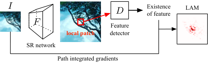

3.3 Local Attribution Maps
In this section, we describe the proposed Local Attribution Maps (LAM), which is based on the integrated gradients method sundararajan2017axiomatic. Let be an SR network with the upscaling factor . As stated before, we interpret by attributing the existence of certain features of local patches in the output image, instead of the pixel intensities. We quantify the existence of a specific feature in an patch located in with a detector . Here, is implemented by simple operators or filters, which can be easily understood, to avoid introducing additional difficulty to the interpretation. In this work, we mainly use the gradient detector to quantify the existence of edges and textures, as
| (1) |
where the subscript indicates the location coordinates. In the following text, we omit the subscripts for convenience without loss of generality. Given as the input LR image, conducting attribution analysis of an SR network also requires a baseline input image , which satisfies that absent certain features existed in . A simple example of is a black image with all zero-value pixels. Accordingly, will show large numerical advantage compared to .
To obtain the attribution map for , we calculate the path integrated gradient along the gradually changing path from to . We represent the path by a smooth path function , where and . Then, the th dimension of the local attribution map is defined as follows:
| (2) |
Obviously, for different baselines and path functions, we obtain different attribution maps. When the baseline inputs are black images and the path function is linear interpolation, Eq (2) degrades to the standard formulation of IG sundararajan2017axiomatic. However, as revealed in sturmfels2020visualizing, the choice of baseline and path function may greatly affect the final attribution results. In this work, we carefully design the baseline inputs and the path function specially for SR networks.
As stated above, a baseline input is meant to represent the “absence” of some input features. In SR, the low-frequency components of the LR image (e.g., color and brightness) contribute less to the final SR performance. In contrast, the high-frequency components (e.g., edges and textures) are of great importance to achieve good SR results. In this work, we design the baseline input by eliminating the high-frequency components. In implementation, we set it as the blurred version of the LR image, denoted as , where represents convolution operation and is the Gaussian blur kernel parameterized by the kernel width . The kernel degrades to the impulse response when equals to 0.
Then we introduce the new path function according to the above baseline input. IG employs linear interpolation function as the path function. However, the linear interpolated images show artifacts and do not follow the prior distribution of natural images. To address this problem, we propose the progressive blurring path function , which achieves a smooth transformation from to through progressively changing the blur kernel:
| (3) |
Obviously, we have and .
In practice, we calculate the gradients at points sampled uniformly along the path and then approximate Eq (2) with a summation:
| (4) | ||||
where is the number of steps in the approximation of the integral. Here, we approximate by calculating the difference after discretization. The calculation of gradients in Eq (4) can be directly implemented using computational graph frameworks, e.g., PyTorch pytorch and Tensorflow tensorflow. Experimentally, a step number of 100 is enough to approximate the integral. One can check the accuracy of the approximation according to the proposition sundararajan2017axiomatic; friedman2004paths that .

3.4 Discussion
Why using integrated gradient. It is counter-intuitive to use the path integrated gradients instead of the vanilla gradients, as the latter one directly indicates the direction of the maximum increase of the detected feature existence. However, the vanilla gradients usually have small magnitudes and fail to indicate important features. This is also called the “gradient saturation”. We illustrate the saturation by plotting the curve of along with the change of . As shown in Figure 3.f, saturation can be triggered when the curve shows a flat trend, where a small shift of along with the gradients does not significantly change the value of . On the contrary, the path integrated gradients shows how changes from small to large and its attribution map indicates the pixels that contribute most significantly to when changing alone the path. We illustrate this process by decomposing Eq (2) into two parts: the gradients at the interpolated images and the gradients of , where the latter one could be viewed as weights for the gradients at different interpolations. As shown in Figure 3.f, the change of is not linear. It experiences a sharp increase in the range marked by the green dashed line. Meanwhile, the magnitudes of also have large values in this range, which makes these gradients provide greater contribution to the final attribution map. We also show the curve of the cumulative gradients over in Figure 3.h. Notice that high magnitude gradients accumulate at the same range where the increases sharply and also where the magnitudes of have large values. These experiments show the rationality of using the path integral gradient instead of the vanilla gradient.
The choice of baseline and path function. Although Sundararajan et al. sundararajan2017axiomatic suggest to use black image as baseline and linear interpolation as the path function, Sturmfels et al. sturmfels2020visualizing argue that it may not be the best choice. We experimentally show its disadvantages in Figure 3. As can be seen, the linear interpolated images of black baseline image does not present the “absence” of important features, although the feature detection output of the baseline image is reduced. It reduces by reducing the intensity of all the pixels, resulting in saturation for the gradients of all these interpolations. On the other hand, is equal to for all in linear path function, which provides all gradients the same weights. For these reasons, the black baseline image and linear path function are not suitable for interpreting the SR networks. Alternative choices are proposed in this work for SR networks. We use a blurred image as baseline to represent the missing high-frequency components. The the progressively blurring function is presented as a natural choice of path function. With the mathematical characteristics of path integral gradients, the proposed method can provide reasonable attribution results for SR networks.


4 Experiments
4.1 Collection of Test Set and Visualization Method
Following the principle of interpreting hard cases, we collect 150 images that are challenging for SR networks as the test set for the following analysis. We first sample more than 30,000 sub-images of size from DIV2K validation set div2k and Urban100 huang2015single and then obtain their SR results using different SR networks. We select the sub-images that have low average PSNR performance and high variance between different SR networks and then manually remove images with duplicate and unidentifiable content. In practice, we only perform attribution analysis to the local patch in the center of the image, so we manually adjust the image to make the content in the center meaningful. In our test set, the average PSNR value is only 20.87dB. Compared with 28.59dB and 24.12dB (the average PSNR values of DIV2K validation set and Urban100), our test images are challenging for SR networks. When selecting metrics for quantitative evaluation, we follow the suggestion of Gu et al. gu2020pipal and employ both PSNR and the LPIPS perceptual similarity zhang2018unreasonable. For the visualization of the attribution results, we first normalize the maps to the range and then take the absolute values. Although the normalization only keeps the relative values without signs, we contend that such properties will not affect the perception of the output visualization. Similar visualization methods are also used in some previous work adebayo2018sanity. In the visualization results, a darker pixel (larger intensity) indicates a larger influence w.r.t. the SR results. In the following texts, the heat maps of distributions are obtained using kernel density estimation kde1.
4.2 Diffusion Index for Quantitative Analysis
As stated above, LAM highlights the pixels which have the greatest impact to the SR results. Theoretically, for the same local patch, if the LAM map involves more pixels or a larger range, it can be considered that the SR network has utilized information from more pixels. For quantitative analysis, we employ the Gini coefficient Gini to indicate the range of involved pixels, denoted as
| (5) |
where represents the absolute value of the th dimension of the attribution map, is the mean value and . Gini coefficient is originally a measure of statistical dispersion intended to represent the income inequality. In our case, the inequality of pixels’ contribution to the attribution result also reflects the range of involved pixels. If a few pixels contribute a large proportion in the total attribution result, its Gini coefficient is relatively high, otherwise, a low Gini coefficient indicates the attribution result involves more pixels. In practice, we rescale the Gini coefficient and propose the diffusion index (DI) to facilitate analysis, denoted as
| (6) |
Notice that in this setting, a larger DI indicates more pixels are involved. We illustrate the Gini and diffusion coefficient in Figure 4 with examples.
4.3 Attribution Results
We show some LAM results of different SR networks in Figure 5. We can have the following observations. First, the early network FSRCNN fsrcnn2016 and shallow network CARN carn2018 have relatively small receptive fields and can only perform SR based on limited surrounding pixels. Deep residual networks, i.e., EDSR edsr2017, RRDBNet wang2018esrgan, RCAN rcan2018 and DRLN drln2020, have deeper architectures and bigger receptive fields. Their LAM results show that these networks are interested in a wider range of pixels in the LR images with similar patterns, e.g., the regular stripes that appear on skyscrapers. Although the textures in these areas are heavily aliased in the LR image, which may mislead the SR process, some networks still reconstruct accurate textures and they, according to the LAM results, take notice of a wider range of unaliased areas. Second, non-local and channel-wise attention modules are introduced to SR networks in recent years, expecting to utilize long-term and global information to assist the SR. Representative network designs include RNAN nonResidual, RCAN and SAN san2019. The proposed LAM method can also be applied to diagnose and visualize that whether global and long-term information is used by these networks. As can be observed from Figure 5, they all extract information from non-local pixels. This experiment demonstrates the value of LAM as a research aid. Third, it’s worth noting that some networks also take a wider range of pixels into account but still reconstruct wrong textures, e.g., SAN and DRLN in the second example. In these models, the information from more pixels is not effectively used for accurate reconstruction.
We then visualize the similarities and differences of LAM results for different SR networks in Figure 6. The heat maps in the third row show the areas of interest for different SR networks. The information carried in the red areas can be used for the most preliminary level of SR, while the blue areas show the potential informative areas that can further improve SR. How to extract and use the information in blue areas is the key factor for a SR network to distinguish with others. To empirically analyze the patterns of information utilization, we find that they are more likely to notice areas with self-similar properties and regular textures. For instance, in the 6th, 7th, and 8th examples of Figure 6, the attention of the SR networks is distributed along the direction of texture extension; and in the 9th example, the SR networks notice the similar-shaped windows around the target patch. We include more results in Appendix C.
| Model | Recpt. Field | PSNR | DI | Remark |
|---|---|---|---|---|
| FSRCNN | 1717 | 20.30 | 0.797 | Fully convolution network. |
| CARN | 4545 | 21.27 | 1.807 | Residual network. |
| EDSR | 7575 | 20.96 | 2.977 | Residual network. |
| MSRN | 107107 | 21.39 | 3.194 | Residual network. |
| RRDBNet | 703703 | 20.96 | 13.417 | Residual network. |
| IMDN | global | 21.23 | 14.643 | Global pooling. |
| RFDN | global | 21.40 | 13.208 | Global pooling. |
| RCAN | global | 22.20 | 16.596 | Global pooling. |
| RNAN | global | 21.91 | 13.243 | Non-local attention. |
| SAN | global | 22.55 | 18.642 | Non-local attention. |
4.4 Exploration with LAM
In this section, we use LAM as a tool to explore SR networks. We study the relationship between the diffusion index of LAM results and several indicators of SR networks, e.g., performance, scales and receptive fields. In our experiment, totally 48 SR networks are collected for analysis, consisting of 18 networks from the literature and 30 networks with different network scales. For networks from the literature, we select: SRCNN srcnn2014, FSRCNN, EDSR, LapSRN lapsrn2017, SRResNet srgan2017, DDBPN ddbpn2018, RDN rdn2018, MSRN msrn2018, RCAN, RRDBNet, CARN, SAN, IMDN imdn2019, RNAN nonResidual, RFDN rfdn2020, PAN pan2020, DRLN, and CSNLN crossNonlocal. For networks with different network scales, we collect networks for two representative architectures, i.e., FSRCNN fsrcnn2016 as a representative of the fully convolution networks and EDSR edsr2017 as a representative of the residual networks. For FSRCNN, the range of width is selected to be and the range of depth is , with 15 models in total. For EDSR, the range of width is selected to be and the range of residual blocks is , with 15 models in total. All the models are trained with the same setting. More details about model collection can be found in Appendix B.
Diffusion Index vs. Network Performances. The question that we are most interested in is “can we get better SR performance by utilizing information from more pixels?” We establish this relationship with linear regression fitting, where the x-axis represents the log number of DI and the y-axis represents the SR performance. We illustrate the results in Figure 7.a and Figure 7.b. The high pearson correlation and spearman correlation (both larger than 0.8) indicate that the extraction of information from a wider range of pixels and SR performance are highly correlated, the two-tailed p-test results for both experiments are lower than . Finding ways to capture the benefits from a wider range of pixels is an important direction for future work.
Diffusion Index vs. Receptive Field. A result of network deepening is the increase of the receptive field, and some networks also propose to increase the receptive field on purpose to promote SR. We are curious whether the increase in the receptive field directly promotes the use of information from a wider range of pixels. In Table 1 we show the receptive fields, PSNR and DI performances for some representative SR networks. As the number of convolution layers increases, the receptive field steadily increases, and the area and pixels that the network can perceive also increase. In addition to adding more convolution layers, channel-wise attention with global pooling layers and non-local operations are also introduced, which can theoretically increase the receptive field to cover the whole image. Compared with RRDBNet (whose receptive field is already larger than the size of the test images), IMDN, RFDN and RNAN with the above global operations do not significantly utilize the information from more pixels. However, they are more efficient in the use of information, which is reflected in their better PSNR performance. Besides, RCAN employs not only global operations but also more than 400 convolution layers that can support a very large effective receptive field, and SAN employs multiple non-local operations and also global-wised attentions. They all achieve higher DI values and also better performances. We argue that the receptive field of the existing networks is large enough, and the effect of simply increasing the receptive field is limited. How to effectively utilize the information within the receptive area pixels is critical.
Diffusion Index vs. Network Scales. SR networks have grown deeper and wider in the quest for higher reconstruction accuracy. We now investigate the relationship between the attribution results and different SR network scales (width and depth). The results are shown in Figure 7.c. As one can observe, with the increase of both depth and width, FSRCNN is able to extract information from more pixels and also achieves better PSNR performance. For EDSR, the increase of the number of convolution layers directly increases the receptive field and leads to better DI values and PSNR performance, however, the increase of the number of feature maps in each layer does not achieve the corresponding improvement. This is because, under the same training condition, networks with larger parameters are difficult to optimize effectively.

Diffusion Index vs. Image Content. We have also observed significant differences in LAM results on images with different content. We first sort the images with highest DI values and the results are shown in Figure 8. As can be observed, the network’s perception of different image contents is also different. In some images, even for the SR network with a large receptive field and good learning capacity, the area of noticing is still narrow. It indicates that these networks believe the semantics or features in a wider area have little help to the SR of the current patch. On the contrary, for some other images, these networks can extract features from a wider surrounding area. We illustrate these two image categories in Figure 8. As can be observed, images with regular stripe and grid textures are very likely to be detected by SR networks, while the complex high-level semantics, such as human and animal, can not be effectively used. The results of LAM actually point out that for SR networks, the extracted and used abstract semantics are different from what people usually understand. It is an open question that whether the use of complex high-level semantics can help SR.
5 Conclusion
In this paper, we propose local attribution map (LAM) to visualize and understand SR networks. We experimentally demonstrate the potential of LAM as a research tool and reveal some interesting conclusions about what information is used by SR networks and how this information affect performance. Our work opens new directions for designing SR networks and interpreting low-level vision deep models.
References
- (1) Martín Abadi, Paul Barham, Jianmin Chen, Zhifeng Chen, Andy Davis, Jeffrey Dean, Matthieu Devin, Sanjay Ghemawat, Geoffrey Irving, Michael Isard, et al. Tensorflow: A system for large-scale machine learning. In 12th USENIX symposium on operating systems design and implementation (OSDI 16), pages 265–283, 2016.
- (2) Julius Adebayo, Justin Gilmer, Ian Goodfellow, and Been Kim. Local explanation methods for deep neural networks lack sensitivity to parameter values. arXiv preprint arXiv:1810.03307, 2018.
- (3) Julius Adebayo, Justin Gilmer, Michael Muelly, Ian Goodfellow, Moritz Hardt, and Been Kim. Sanity checks for saliency maps. In Advances in Neural Information Processing Systems, pages 9505–9515, 2018.
- (4) Eirikur Agustsson and Radu Timofte. Ntire 2017 challenge on single image super-resolution: Dataset and study. In Proceedings of the IEEE Conference on Computer Vision and Pattern Recognition Workshops, pages 126–135, 2017.
- (5) Namhyuk Ahn, Byungkon Kang, and Kyung-Ah Sohn. Fast, accurate, and lightweight super-resolution with cascading residual network. In Proceedings of the European Conference on Computer Vision (ECCV), pages 252–268, 2018.
- (6) Marco Ancona, Enea Ceolini, Cengiz Öztireli, and Markus Gross. Towards better understanding of gradient-based attribution methods for deep neural networks. In International Conference on Learning Representations, 2018.
- (7) Saeed Anwar and Nick Barnes. Densely residual laplacian super-resolution. IEEE Transactions on Pattern Analysis and Machine Intelligence, 2020.
- (8) André Araujo, Wade Norris, and Jack Sim. Computing receptive fields of convolutional neural networks. Distill, 4(11):e21, 2019.
- (9) Sebastian Bach, Alexander Binder, Grégoire Montavon, Frederick Klauschen, Klaus-Robert Müller, and Wojciech Samek. On pixel-wise explanations for non-linear classifier decisions by layer-wise relevance propagation. PloS one, 10(7):e0130140, 2015.
- (10) David Baehrens, Timon Schroeter, Stefan Harmeling, Motoaki Kawanabe, Katja Hansen, and Klaus-Robert Müller. How to explain individual classification decisions. The Journal of Machine Learning Research, 11:1803–1831, 2010.
- (11) David Bau, Jun-Yan Zhu, Hendrik Strobelt, Bolei Zhou, Joshua B Tenenbaum, William T Freeman, and Antonio Torralba. Gan dissection: Visualizing and understanding generative adversarial networks. In International Conference on Learning Representations, 2018.
- (12) Alexander Binder, Grégoire Montavon, Sebastian Lapuschkin, Klaus-Robert Müller, and Wojciech Samek. Layer-wise relevance propagation for neural networks with local renormalization layers. In International Conference on Artificial Neural Networks, pages 63–71. Springer, 2016.
- (13) Tao Dai, Jianrui Cai, Yongbing Zhang, Shu-Tao Xia, and Lei Zhang. Second-order attention network for single image super-resolution. In Proceedings of the IEEE conference on computer vision and pattern recognition, pages 11065–11074, 2019.
- (14) Chao Dong, Chen Change Loy, Kaiming He, and Xiaoou Tang. Image super-resolution using deep convolutional networks. IEEE transactions on pattern analysis and machine intelligence, 38(2):295–307, 2015.
- (15) Chao Dong, Chen Change Loy, and Xiaoou Tang. Accelerating the super-resolution convolutional neural network. In European conference on computer vision, pages 391–407. Springer, 2016.
- (16) Ruth Fong, Mandela Patrick, and Andrea Vedaldi. Understanding deep networks via extremal perturbations and smooth masks. In Proceedings of the IEEE International Conference on Computer Vision, pages 2950–2958, 2019.
- (17) Ruth C Fong and Andrea Vedaldi. Interpretable explanations of black boxes by meaningful perturbation. In Proceedings of the IEEE International Conference on Computer Vision, pages 3429–3437, 2017.
- (18) Eric J Friedman. Paths and consistency in additive cost sharing. International Journal of Game Theory, 32(4):501–518, 2004.
- (19) Jinjin Gu, Haoming Cai, Haoyu Chen, Xiaoxing Ye, Jimmy Ren, and Chao Dong. Pipal: a large-scale image quality assessment dataset for perceptual image restoration. In European conference on computer vision. Springer, 2020.
- (20) Jinjin Gu, Hannan Lu, Wangmeng Zuo, and Chao Dong. Blind super-resolution with iterative kernel correction. In Proceedings of the IEEE Conference on Computer Vision and Pattern Recognition, pages 1604–1613, 2019.
- (21) Muhammad Haris, Gregory Shakhnarovich, and Norimichi Ukita. Deep back-projection networks for super-resolution. In Proceedings of the IEEE conference on computer vision and pattern recognition, pages 1664–1673, 2018.
- (22) Kaiming He, Xiangyu Zhang, Shaoqing Ren, and Jian Sun. Deep residual learning for image recognition. In Proceedings of the IEEE conference on computer vision and pattern recognition, pages 770–778, 2016.
- (23) Gao Huang, Zhuang Liu, Laurens Van Der Maaten, and Kilian Q Weinberger. Densely connected convolutional networks. In Proceedings of the IEEE conference on computer vision and pattern recognition, pages 4700–4708, 2017.
- (24) Jia-Bin Huang, Abhishek Singh, and Narendra Ahuja. Single image super-resolution from transformed self-exemplars. In Proceedings of the IEEE conference on computer vision and pattern recognition, pages 5197–5206, 2015.
- (25) Zheng Hui, Xinbo Gao, Yunchu Yang, and Xiumei Wang. Lightweight image super-resolution with information multi-distillation network. In Proceedings of the 27th ACM International Conference on Multimedia, pages 2024–2032, 2019.
- (26) Jiwon Kim, Jung Kwon Lee, and Kyoung Mu Lee. Accurate image super-resolution using very deep convolutional networks. In Proceedings of the IEEE conference on computer vision and pattern recognition, pages 1646–1654, 2016.
- (27) Jiwon Kim, Jung Kwon Lee, and Kyoung Mu Lee. Deeply-recursive convolutional network for image super-resolution. In Proceedings of the IEEE conference on computer vision and pattern recognition, pages 1637–1645, 2016.
- (28) Diederik P Kingma and Jimmy Ba. Adam: A method for stochastic optimization. arXiv preprint arXiv:1412.6980, 2014.
- (29) Wei-Sheng Lai, Jia-Bin Huang, Narendra Ahuja, and Ming-Hsuan Yang. Deep laplacian pyramid networks for fast and accurate super-resolution. In Proceedings of the IEEE conference on computer vision and pattern recognition, pages 624–632, 2017.
- (30) Christian Ledig, Lucas Theis, Ferenc Huszár, Jose Caballero, Andrew Cunningham, Alejandro Acosta, Andrew Aitken, Alykhan Tejani, Johannes Totz, Zehan Wang, et al. Photo-realistic single image super-resolution using a generative adversarial network. In Proceedings of the IEEE conference on computer vision and pattern recognition, pages 4681–4690, 2017.
- (31) Juncheng Li, Faming Fang, Kangfu Mei, and Guixu Zhang. Multi-scale residual network for image super-resolution. In Proceedings of the European Conference on Computer Vision (ECCV), pages 517–532, 2018.
- (32) Bee Lim, Sanghyun Son, Heewon Kim, Seungjun Nah, and Kyoung Mu Lee. Enhanced deep residual networks for single image super-resolution. In Proceedings of the IEEE conference on computer vision and pattern recognition workshops, pages 136–144, 2017.
- (33) Ding Liu, Bihan Wen, Yuchen Fan, Chen Change Loy, and Thomas S Huang. Non-local recurrent network for image restoration. In Advances in Neural Information Processing Systems, pages 1673–1682, 2018.
- (34) Jie Liu, Jie Tang, and Gangshan Wu. Residual feature distillation network for lightweight image super-resolution. In European Conference on Computer Vision Workshop (ECCVW). Springer, 2020.
- (35) Scott M Lundberg and Su-In Lee. A unified approach to interpreting model predictions. In Advances in neural information processing systems, pages 4765–4774, 2017.
- (36) Aravindh Mahendran and Andrea Vedaldi. Visualizing deep convolutional neural networks using natural pre-images. International Journal of Computer Vision, 120(3):233–255, 2016.
- (37) Yiqun Mei, Yuchen Fan, Yuqian Zhou, Lichao Huang, Thomas S Huang, and Honghui Shi. Image super-resolution with cross-scale non-local attention and exhaustive self-exemplars mining. In Proceedings of the IEEE/CVF Conference on Computer Vision and Pattern Recognition, pages 5690–5699, 2020.
- (38) Emanuel Parzen. On estimation of a probability density function and mode. The annals of mathematical statistics, 33(3):1065–1076, 1962.
- (39) Adam Paszke, Sam Gross, Francisco Massa, Adam Lerer, James Bradbury, Gregory Chanan, Trevor Killeen, Zeming Lin, Natalia Gimelshein, Luca Antiga, et al. Pytorch: An imperative style, high-performance deep learning library. In Advances in neural information processing systems, pages 8026–8037, 2019.
- (40) Guocheng Qian, Jinjin Gu, Jimmy S Ren, Chao Dong, Furong Zhao, and Juan Lin. Trinity of pixel enhancement: a joint solution for demosaicking, denoising and super-resolution. arXiv preprint arXiv:1905.02538, 2019.
- (41) Ramprasaath R Selvaraju, Michael Cogswell, Abhishek Das, Ramakrishna Vedantam, Devi Parikh, and Dhruv Batra. Grad-cam: Visual explanations from deep networks via gradient-based localization. In Proceedings of the IEEE international conference on computer vision, pages 618–626, 2017.
- (42) Junghoon Seo, Jeongyeol Choe, Jamyoung Koo, Seunghyeon Jeon, Beomsu Kim, and Taegyun Jeon. Noise-adding methods of saliency map as series of higher order partial derivative. arXiv preprint arXiv:1806.03000, 2018.
- (43) Yujun Shen, Jinjin Gu, Xiaoou Tang, and Bolei Zhou. Interpreting the latent space of gans for semantic face editing. In Proceedings of the IEEE/CVF Conference on Computer Vision and Pattern Recognition, pages 9243–9252, 2020.
- (44) Wenzhe Shi, Jose Caballero, Ferenc Huszár, Johannes Totz, Andrew P Aitken, Rob Bishop, Daniel Rueckert, and Zehan Wang. Real-time single image and video super-resolution using an efficient sub-pixel convolutional neural network. In Proceedings of the IEEE conference on computer vision and pattern recognition, pages 1874–1883, 2016.
- (45) Avanti Shrikumar, Peyton Greenside, and Anshul Kundaje. Learning important features through propagating activation differences. In International Conference on Machine Learning, pages 3145–3153, 2017.
- (46) Avanti Shrikumar, Peyton Greenside, Anna Shcherbina, and Anshul Kundaje. Not just a black box: Learning important features through propagating activation differences. arXiv preprint arXiv:1605.01713, 2016.
- (47) Karen Simonyan, Andrea Vedaldi, and Andrew Zisserman. Deep inside convolutional networks: Visualising image classification models and saliency maps. arXiv preprint arXiv:1312.6034, 2013.
- (48) Daniel Smilkov, Nikhil Thorat, Been Kim, Fernanda Viégas, and Martin Wattenberg. Smoothgrad: removing noise by adding noise. arXiv preprint arXiv:1706.03825, 2017.
- (49) J Springenberg, Alexey Dosovitskiy, Thomas Brox, and M Riedmiller. Striving for simplicity: The all convolutional net. In ICLR (workshop track), 2015.
- (50) Pascal Sturmfels, Scott Lundberg, and Su-In Lee. Visualizing the impact of feature attribution baselines. Distill, 5(1):e22, 2020.
- (51) Mukund Sundararajan, Ankur Taly, and Qiqi Yan. Axiomatic attribution for deep networks. In International Conference on Machine Learning, pages 3319–3328, 2017.
- (52) Ying Tai, Jian Yang, and Xiaoming Liu. Image super-resolution via deep recursive residual network. In Proceedings of the IEEE conference on computer vision and pattern recognition, pages 3147–3155, 2017.
- (53) Tong Tong, Gen Li, Xiejie Liu, and Qinquan Gao. Image super-resolution using dense skip connections. In Proceedings of the IEEE International Conference on Computer Vision, pages 4799–4807, 2017.
- (54) Xiaolong Wang, Ross Girshick, Abhinav Gupta, and Kaiming He. Non-local neural networks. In Proceedings of the IEEE conference on computer vision and pattern recognition, pages 7794–7803, 2018.
- (55) Xintao Wang, Ke Yu, Chao Dong, and Chen Change Loy. Recovering realistic texture in image super-resolution by deep spatial feature transform. In Proceedings of the IEEE Conference on Computer Vision and Pattern Recognition, pages 606–615, 2018.
- (56) Xintao Wang, Ke Yu, Shixiang Wu, Jinjin Gu, Yihao Liu, Chao Dong, Yu Qiao, and Chen Change Loy. Esrgan: Enhanced super-resolution generative adversarial networks. In European Conference on Computer Vision, pages 63–79. Springer, 2018.
- (57) Shlomo Yitzhaki. Relative deprivation and the gini coefficient. The quarterly journal of economics, pages 321–324, 1979.
- (58) Richard Zhang, Phillip Isola, Alexei A Efros, Eli Shechtman, and Oliver Wang. The unreasonable effectiveness of deep features as a perceptual metric. In Proceedings of the IEEE Conference on Computer Vision and Pattern Recognition, pages 586–595, 2018.
- (59) Yulun Zhang, Kunpeng Li, Kai Li, Lichen Wang, Bineng Zhong, and Yun Fu. Image super-resolution using very deep residual channel attention networks. In Proceedings of the European Conference on Computer Vision (ECCV), pages 286–301, 2018.
- (60) Yulun Zhang, Kunpeng Li, Kai Li, Bineng Zhong, and Yun Fu. Residual non-local attention networks for image restoration. arXiv preprint arXiv:1903.10082, 2019.
- (61) Yulun Zhang, Yapeng Tian, Yu Kong, Bineng Zhong, and Yun Fu. Residual dense network for image super-resolution. In Proceedings of the IEEE conference on computer vision and pattern recognition, pages 2472–2481, 2018.
- (62) Hengyuan Zhao, Xiangtao Kong, Jingwen He, Yu Qiao, and Chao Dong. Efficient image super-resolution using pixel attention. In European Conference on Computer Vision Workshop (ECCVW). Springer, 2020.
- (63) Bolei Zhou, David Bau, Aude Oliva, and Antonio Torralba. Interpreting deep visual representations via network dissection. IEEE transactions on pattern analysis and machine intelligence, 41(9):2131–2145, 2018.
- (64) Bolei Zhou, Aditya Khosla, Agata Lapedriza, Aude Oliva, and Antonio Torralba. Learning deep features for discriminative localization. In Proceedings of the IEEE conference on computer vision and pattern recognition, pages 2921–2929, 2016.
Appendix
Appendix A Review of Attribution Methods
In this section, we provide a review of attribution methods in the literature that are used for interpreting classification networks. We also discuss their relationship with the interpretation of super-resolution (SR) networks. Given an input image and a model that outputs the probability of belongs to a certain class, an attribution method provides attribution maps for that are of the same size as the inputs. Each dimension of these attribution maps corresponds to the “relevance” or “importance” of that dimension to the final output, which is often a class-specific score in classification networks.
Gradient w.r.t. . This method employs the gradient of the predicted probability w.r.t. to the input simonyan2013deep; baehrens2010explain.
| (7) |
However, the vanilla gradient method suffers from the “saturation” problem that the magnitude of this gradient tends to be small. A little movement toward the direction of the gradient will not change the predicted probability significantly sturmfels2020visualizing. In Sec 3.4, we show that for the interpretation of SR networks, the “saturation” problem also exist. Thus the vanilla gradient method is not appropriate for interpreting SR networks.
The element-wise product of Gradient and the input. This method was proposed to address the saturation problem and reduce visual diffusion shrikumar2016not, denoted as
| (8) |
Ancona et al. ancona2018towards show that, for a network with only ReLU activation function and no additive biases, this input gradient product is equivalent to DeepLift shrikumar2016not, and -LRP bach2015pixel. For the interpretation of SR networks, the pixel intensity should not be part of the attribution as the textures and edges may not change when the pixel intensity changes. Directly calculate the product of the input intensity and the gradient will introduce interference factors.
Guided Backpropagation (GBP). This method specifies a change in how to calculate gradients for ReLU activations. Let be the feature maps obtained during the forward process by a deep neural network , and be the representation obtained during the backward process. Springenberg et al. springenberg2015striving propose GBP that aims to zero out negative gradients during the computation of . The map is computed as:
| (9) |
where represents keeping only the positive gradients and indicates keeping only the positive activations. The usage scenarios of this method are relatively limited. For residual networks that are widely used in SR, this method is not valid.
Integrated Gradients (IG). Most relevant to the method proposed in this paper, IG also employs path integration friedman2004paths, but uses a black image as baseline image and linear interpolation as the path function. IG is defined as:
| (10) |
where is the baseline black image and is the parameter of the interpolation. In Sec 3.4, we discuss the differences between the proposed local attribution maps for SR networks and IG.
SmoothGrad and VarGrad. SmoothGrad smilkov2017smoothgrad and VarGrad adebayo2018local are proposed to relieve the situation where the attribution graph is full of noise. The SmoothGrad is defined as:
| (11) |
where are the noise vectors and are sampled from a Gaussian distribution. Similar to SmoothGrad, a variance analog of SmoothGrad can be defined as:
| (12) |
where represents to the variance. Seo et al. seo2018noise theoretically analyze VarGrad showing that it is independent of the gradient, and captures higher order partial derivatives. For SR networks, adding noise to the input is destructive to the output image qian2019trinity; gu2019blind. Thus both SmoothGrad and VarGrad can not be used to interpret SR networks. On the other hand, SmoothGrad and VarGrad also face the challenge of gradient saturation.
CAM, GradCAM and Guided GradCAM. Different from the aforementioned gradient-based attribution methods, Class Activation Mapping (CAM) zhou2016learning generates class activation maps using the global average pooling in convolution neural networks. A CAM map for a particular category indicates the discriminative image regions used by the network to identify that category. Combining gradient-based methods and CAM, Selvaraju et al. selvaraju2017grad further propose GradCAM that corresponds to the gradient of the class score w.r.t. the feature map of the last convolution unit. For pixel level granularity, GradCAM can be combined with Guided Backpropagation through an element-wise product. Since CAM is specially designed for high-level vision networks with global pooling layers, it cannot be easily adapted to low-level vision models such as SR networks.
Perturbation-Based Methods. Different from the above works that require the mathematical details of the model, there are works that treat deep models as black-boxes. These methods usually localize the discriminative image regions by performing perturbation to the input. For instance, Fong and Vedaldi fong2017interpretable propose to explain neural networks that are based on learning the minimal deletion to an image that changes the model prediction. Similar to SmoothGrad and VarGrad, the sensitivity of SR networks to disturbances and perturbation makes it difficult to use these approach to explain.
Appendix B Collection of Models
In this section, we first describe the training settings in our experiments and then briefly review the used SR networks. We use DIV2K training set div2k for training and the size of LR image is . For optimization, we use Adam kingma2014adam with the default settings that and . The learning rate is initialized as and decayed linearly at every updates. The size of minibatch is set to 16. We next briefly review the used SR networks.
Early methods with fully convolutional architectures. These methods include SRCNN srcnn2014, FSRCNN fsrcnn2016 and ESPCN espcn2016. What they have in common is that they only use stacked convolution layers without residual or other deep modules. SRCNN is the first deep SR network that consists of only three convolution layers without upsampling layer – it takes the bicubic interpolation result as input. FSRCNN consists of eight convolution layers and uses deconvolution layer as the upsampling layer. In ESPCN, pixel shuffle is used innovatively as an upsampling operation, and this operation is used on a large scale by subsequent SR networks. In addition to the above networks, DDBPN ddbpn2018 and LapSRN lapsrn2017 are also in the form of fully convolution networks with different convolution strategies. LapSRN is a network with progressive upsampling operations that super-resolves low-resolution images in a coarse-to-fine laplacian pyramid framework. DDBPN exploits iterative up- and downsampling layers, aiming at providing an error feedback mechanism for projection errors at each stage.
Networks with residual and dense connections. These methods date back to SRResNet srgan2017 that first introduce residual connections he2016deep to deep SR networks. Some methods are proposed to improve the residual structure such as EDSR edsr2017, CARN carn2018 and MSRN msrn2018. Spatial feature transformation blocks are also introduced to SR networks sftgan2018; gu2019blind to achieve interactive SR. Inspired by dense connection network huang2017densely, RDN rdn2018 and SRDenseNet srdense2017 with dense architecture was proposed. Combining residual blocks and dense connections, residual-in-residual dense net (RRBDNet) wang2018esrgan was proposed. Recently, DRLN drln2020 employs cascading residual on the residual structure to allow the flow of low-frequency information to focus on learning high and mid-level features.
Networks with attention modules. In addition to innovations in various short connections, attention modules are also used to improve the performance of SR networks. Zhang et al. rcan2018 propose channel attention that compute attention weights w.r.t. the whole channel. Zhao et al. pan2020 propose pixel attention that compute attention weights using convolution for each pixel. Non-local operation is also introduced in the form of attention module in nonResidual; nonRecurrent. SAN san2019 utilizes both non-local attention modules and second-order channel attention. Recently, CSNLN crossNonlocal employs cross-scale non-Local attention module with integration into a recurrent neural network to learn cross-scale feature correlation.
Appendix C More Results
In this section, we exhibit more results. We first show more examples of the “area of interest”. In Figure 6, we have shown the five images with the smallest area of interest and also five images with the largest area of interest. In Figure 9, we show more images with their area of interest and the rank indices are also marked. In Figure 10, Figure 11, Figure 12, and Figure 13, we show more LAM results.
Appendix D Change Log
v1 initial pre-print release.
v2 We correct a typo that there should not be a at the end of Eq (4). There is no such problem with the code. The conclusions of this paper are not affected.


