Tunable Tradeoff between Quantum and Classical Computation via Nonunitary Zeno-like Dynamics

Quantum measurement has been proven to be a powerful tool that not only allows us to learn about a quantum system but also to control its state. It plays a fundamental role in quantum information with applications, among many other things, ranging from quantum communications to quantum algorithms. The quantum Zeno effect (QZE) is a widely-employed technique for quantum control, which is based on repeated frequent measurements of the entire system or part of it Facchi and Pascazio 2008a. A number of studies have employed the QZE or similar techniques for various flavours of search problems Rudolph and Grover 2002; Childs et al. 2002; Hosten et al. 2006, to establish remarkable relations between the efficiency of quantum and associated classical algorithms Lin and Lin 2015, as well as singular value transformations Gilyén et al. 2019. The Zeno dynamics of a closed quantum system induced by projective measurement will yield unitary dynamics, but the evolution due to observation may be more general. Measurement-induced nonunitary dynamics have been considered in the literature both as primitives Knill et al. 2001; Terashima and Ueda 2005; Kendon and Sanders 2005; Kendon and Maloyer 2008; Usher et al. 2017, or as essential ingredients of specific protocols Nakazato et al. 2003; Wu et al. 2004; Li et al. 2011; Pyshkin et al. 2016; Pyshkin et al. 2021; Luchnikov and Filippov 2017; Streltsov et al. 2011; Gilyén et al. 2015; Coles and Piani 2014; Torres et al. 2017; Pyshkin et al. 2017; Grimaudo et al. 2020. Another source of nonunitary evolution may be a special coupling with environment Amin et al. 2008; Luo et al. 2015; Novo et al. 2018.

In this paper, we consider an algorithm that is a variant of the continuous search algorithm introduced by Farhi and Gutmann Farhi and Gutmann 1998. This algorithm follows a scheme based on the combination of time-dependent measurement and Hamiltonian evolution of the system Nakazato et al. 2003, admitting a nonunitary description and exhibiting a non-periodic time dependence of the target fidelity. Our approach is based on repeated measurements and post-selection, therefore the survival probability associated with successfully completing the desired number of steps may be less than one, in addition to the usual probability related to the target fidelity. We show that in the case of a detuned oracle, the target fidelity can be increased up to unity at the expense of the survival probability, which makes it a favourable choice in situations where the correctness of the obtained result cannot be easily verified. While the algorithm is interesting in its own right, it is remarkable that our measurement-based algorithm is robust and self-protected against a certain class of noises Wu and Byrd 2008; Lidar and Wu 2003. This robustness can be attributed to the noise suppression of the repeated measurements. The algorithm provides a framework for studying the trade-off between quantum and classical computation, where the quantum speedup is related to the unitary operations while measurements lead to the appearance of classical probabilities for different outcomes. Thus, in order to combine classical and quantum computations in a single process, one can consider unitary dynamics interrupted by selective measurements.

We start from the continuous-time Grover search algorithm described by the Hamiltonian in the Hilbert space $\mathcal{H}_{N}$ ($\dim\mathcal{H}_{N}=N$),

where $\ket{s}=\sum_{n}^{N}\ket{n}/\sqrt{N}$ and $\ket{w}$ denotes the marked element in the database. Taking $\ket{\psi(0)}=\ket{s}$ as the initial state the evolution remains in a two-dimensional subspace of the total Hilbert space spanned by the basis vectors $\{\ket{w},\ket{r}\}$, where $\ket{r}=(\ket{s}-x\ket{w})/\sqrt{1-x^{2}}$, and $x=1/\sqrt{N}$. The evolution of the initial state is given by Farhi and Gutmann 1998

where we have taken $\hbar=1$ for convenience. As follows from (2) the probability to have the system in the target state $\ket{w}$ oscillates in time, with maxima at $T_{j}=\pi x^{-1}(1/2+j)\propto\sqrt{N}$, where $j=0,1,2,\dots$. This periodic behavior is a consequence of the unitarity of the evolution. We stress here that issue of this periodic behaviour can also be tacked by adiabatic quantum search algorithms Farhi et al. 2000; Roland and Cerf 2002, as well as sophisticated time-dependent protocols Pérez and Romanelli 2007; Li et al. 2018.

It is well known that the nonunitary dynamics of quantum systems can have an asymptotic steady state instead of non-damping oscillations (see e.g. Ref. Wu et al. 2004; Li et al. 2011; Luchnikov and Filippov 2017; Pyshkin et al. 2021). We have designed a modification of this algorithm so that $\ket{w}$ becomes such a steady-state.

Let us introduce our nonunitary protocol. We add a qubit ancilla to our system and extend its Hamiltonian to

with $\mathcal{I}$ and $\sigma_{z}$ being the identity and Z-Pauli matrices acting in a space $\mathcal{H}_{A}=\{\ket{\uparrow},\ket{\downarrow}\}$ of the ancilla qubit. Thus the joint Hilbert space now is $\mathcal{H}_{A}\otimes\mathcal{H}_{N}$. We underline here that the interaction between oracle and ancilla “does not know” about $\ket{w}$ state.

We consider the continuous evolution interrupted by projective measurements. The $n$-th step of the protocol of nonunitary evolution is the following:

1. 1)

   The initial state of joint system is $\ket{q_{n-1}}\otimes\ket{\psi_{n-1}}$, where ancilla state $\ket{q_{n-1}}=\cos\theta_{n-1}\ket{\uparrow}+\sin\theta_{n-1}\ket{\downarrow}$

2. 2)

   The joint system evolves time $\delta t$ driven by Hamiltonian (3). It is worth noting that $\delta t$ is not necessarily small, but we assume $\delta t\ll T_{0}$.

3. 3)

   One performs projection measurement $\ket{q_{n}}\bra{q_{n}}$ on the ancilla, where $\ket{q_{n}}=\cos(\theta_{n-1}+\delta\theta)\ket{\uparrow}+\sin(\theta_{n-1}+\delta\theta)\ket{\downarrow}$, where $\delta\theta=\alpha x\delta t\ll 1$, with $\alpha$ being a tunable parameter.

4. 4)

   A successful outcome occurs with probability $p_{n}$, and one leaves the state of joint system in the state $\ket{q_{n}}\otimes\ket{\psi_{n}}$. Otherwise, an unsuccessful outcome indicates that this run of the algorithm must be aborted.

5. 5)

   Let $\theta_{n}=\theta_{n-1}+\delta\theta$

See Fig. 1 for a circuit diagram representation of the complete algorithm. We would like to point out that the algorithm does not require reinitialization of the ancilla qubit after each measurement to some initial state, and this can be considered an advantage.

The Hamiltonian in Eq. (3) can describe single charged spin-$1/2$ particle on a complete graph Salerno 1995 with unconstrained and spin-dependent hopping Jacko et al. 2017, with $w$ corresponding to some unknown vertex where the electrostatic gate is applied (see Fig. 2). In such case, Eq. (3) can be rewritten as $H=-c^{\dagger}_{w\uparrow}c_{w\uparrow}-c^{\dagger}_{w\downarrow}c_{w\downarrow}-\sum_{i\neq j}(c^{\dagger}_{i\uparrow}c_{j\uparrow}-c^{\dagger}_{i\downarrow}c_{j\downarrow})$, where $c_{i\uparrow(\downarrow)}$ is annihilation operator for the particle on site $i$ with spin $\uparrow(\downarrow)$. In this setting, the spin degree of freedom acts as ancilla.

Another way to implement the Hamiltonian (3) (at least as a proof of concept) with the common quantum circuit model is to use a Trotterization technique Lloyd 1996; Wu et al. 2002; Smith et al. 2019; Tacchino et al. 2020. In this approach we can use the Trotter formula

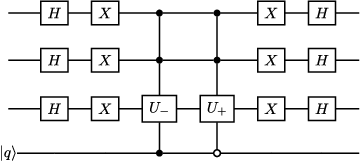
For real simulations, one should use some finite value of $m$ in (4). In order to implement the unitary operation for the first multiplier in the round brackets (oracle) in (4) one can use the algorithm depicted in Fig. 3, while for the second one (diffusion operator) one can use the algorithm depicted in Fig. 4.

The stroboscopic dynamics described above corresponds to a transformation of the initial state $\ket{s}$ by a nonunitary operator $V(n)$ via

where

Note, that the terms in the above product are ordered from right to left. The survival probability $P(n)$ of $n$ first steps is hence given by $P(n)=p_{1}p_{2}\dots p_{n}=\braket{s|V(n)^{\dagger}V(n)|s}$. Equations (5) and (6) can be considered as a set of POVM measurements in the Hilbert space of the oracle. One can add operators $V^{\prime}_{j}=\braket{q^{\perp}_{j}|e^{-iH\delta t}|q_{j-1}}$ with $\ket{q^{\perp}_{j}}=\sin(\theta_{j})\ket{\uparrow}-\cos(\theta_{j})\ket{\downarrow}$ to have a full set of POVM operators for each step $\{V_{j}^{\dagger}V_{j},V^{\prime\dagger}_{j}V^{\prime}_{j}\}$. It is easy to check $V_{j}^{\dagger}V_{j}+V^{\prime\dagger}_{j}V^{\prime}_{j}=\mathbb{I}$. We define the target fidelity at step $n$ as $f(n)=|\braket{w|\psi_{n}}|^{2}$. Together with survival probability $P(n)$ these are the main characteristics of our nonunitary process.

Exact analytic calculation of $V(n)$ in (6) is difficult, however, at first we can note that Hamiltonian (3) has a block-diagonal structure and the calculation of a single $\delta t$ step is an easy task. Taking $\theta_{0}=0$ we obtain the expression

with $C_{j}=\cos((j-1)\delta\theta)\cos(j\delta\theta)$ and $S_{j}=\sin((j-1)\delta\theta)\sin(j\delta\theta)$.

Assuming $x\rightarrow 0$ and $x\delta t\ll 1$ (but finite $\delta t$) we can write, up to a global phase,

Further we consider $\delta\theta\ll 1$. There are special values of $\delta t$ corresponding to $\exp(-2i\delta t)=1$

when each term $V_{j}$ can be approximated by a rescaled unitary, hence the same will hold for the whole process $V(n)$.

As a measure of (non-)unitarity we use the distance

employing the Frobenius norm. We can use this measure to track the trade-off between the unitarity (i.e. quantum computation) and non-unitarity (i.e. classical computation) of the process.

To illustrate the analytical result (9) we plot in Fig. 5 the dependence of $d(V)$ of the resulting transformation $V(n_{G})$ (with $n_{G}=\lfloor\pi\sqrt{N}/(2\delta t)\rfloor$) for various values of $\delta t$ with $N=10^{10}$ and $\delta\theta/\delta t=3\times 10^{-6}$. The minima can be determined from Eq. (9), which involves neither the parameter $\delta\theta$, nor the index $j$.

For further analysis let us define a non-hermitian effective Hamiltonian $H_{\mathrm{eff}}(t)$ by taking the formula

for each $j$, and extending $H_{\mathrm{eff}}(t)$ as piecewise constant on the intervals $((j-1)\delta t,j\delta t]$. The resulting time-dependent (non-hermitian) Hamiltonian provides an equivalent description of the search algorithm.

Introducing the parameter $\tau$ which describes the level of non-unitarity as $\delta t=\pi k+\tau$, for some integer $k$, and assuming $|\tau|\ll 1$ we can approximate the piecewise constant non-hermitian Hamiltonian by the continuous expression

where $\alpha x=\delta\theta/\delta t$. We note that when $\tau=0$ the right hand side becomes hermitian, thus the formal expression $V(n)\approx\mathcal{T}\exp(-i\int_{0}^{n\delta t}H_{\mathrm{eff}}(t^{\prime})dt^{\prime})$ permits an approximation by purely unitary dynamics,

Note, that in the limit $\delta\theta\rightarrow 0$ we have $A(n)=xn\delta t$, yielding the standard continuous Grover algorithm with $f(n)=\sin^{2}(xn\delta t)$. The first maximum occurs at time $T_{0}=n_{G}\delta t=\pi\sqrt{N}/2$, while for $\delta\theta/\delta t=x$ the first maximum is reached at time $\pi\sqrt{N}$. In Fig. 6 we plot some numerical examples.

At non-zero values of $\tau$ we expect the non-hermitian component to drive the system to a steady-state. Of particular interest is the emergence of an asymptotic dynamics consisting of the target state $\ket{w}$ alone, manifesting in the saturation of the target fidelity at the value of $1$. A heuristic analysis of the Hamiltonian (12) shows that in order to achieve saturation dynamics of the fidelity, the relation $\sqrt{x\delta t}\ll\tau\ll 1$ must hold between control parameters (see Appendix for details).

It’s worth pointing out that in our algorithm, when we choose $\theta_{0}=\pi/4$ and $\delta t=\pi/2+\pi k$, $k=0,1,2,\dots$, the first iteration of our algorithm may be approximately described via $V_{1}\approx\ket{w}\bra{w}$ (up to corrections of order $x\delta t\ll 1$). In this situation we would have a classical search regime, i.e. we can organize projection onto the unknown state $\ket{w}$, and the probability of a successful outcome of the ancilla measurement for initial state $\ket{s}$ is $\braket{s|V_{1}^{\dagger}V_{1}|s}\approx 1/N$, which corresponds to the efficiency of the classical search $O(N)$. This example demonstrates the possibility of a classical computation regime which is the opposite of the quantum limit discussed after Eq. (13). Thus we have shown that the proposed algorithm contains quantum, classical and intermediate regimes depending on the parameters chosen.

To study the scaling properties of our nonunitary dynamics we investigate the following transformation of the Hamiltonian (12): $xt=t^{\prime}$, $H^{\prime}(t^{\prime})=H(t)/x$ while keeping $x\delta t$ and $\tau$ constant, and assuming $x\delta t\ll 1$. The last condition here can be approximately satisfied by properly choosing both $N\gg 1$ and an integer $k$. If we have $V(n)$ for some $N=N_{1}$ and $\delta t_{1}=k_{1}\pi+\tau$, then we can find $N_{2}>N_{1}$ and $\delta t_{2}=k_{2}\pi+\tau$ which corresponds to approximately the same operator $V(n)$ when $k_{2}$ is an integer such that

This means that we have almost the same number of steps of the protocol for different $N$, and the duration $\delta t$ of each step is proportional to $\sqrt{N}$. As can be seen, the needed relative accuracy of timing $\tau/\delta t\propto 1/\sqrt{N}$ grows with $N$.

The recurrence relation Eq. (14) can be used to characterize the scaling properties of the algorithm. Assume that we have a certain process with fidelity $f_{1}(t)$, survival probability $P_{1}(t)$, and this process is characterized by $N_{1}$, $\delta t_{1}$, and $\delta\theta_{1}$. We argue that for any requested database size $N_{r}\gg N_{1}$ we can find database size $N_{2}\geq N_{r}$ with corresponding parameters $\delta t_{2}$, $\delta\theta_{2}$ to have another process with $f_{2}(t)$ and $P_{2}(t)$ which is an approximately time scaled copy of the first process with $\delta t_{2}\approx\delta t_{1}\sqrt{N_{2}/N_{1}}$:

and as can be seen $N_{2}/N_{r}\rightarrow 1$ with $N_{r}/N_{1}\rightarrow\infty$.

For a numerical example we chose $N=10^{6}$ and $\alpha=0.3$, $\tau=0.2$, $k=1$, $\delta t=k\pi+\tau$ as a reference process which gives desired $V(n)$. Using (17) we find larger database size ( $N_{r}=10^{18}$), and corresponding integer value of the parameter $k$ which gives the same $V(n_{G})$ as our reference process ($n_{G}=\lfloor\pi\sqrt{N}/(2\delta t)\rfloor$ is the number of steps corresponing to $T_{0}$). The resulting processes are depicted in Fig. 7. Note, the expression (14) is not satisfied exactly for the process (b) in Fig. 7. For requested $N_{r}=10^{18}$ we have $N_{2}=1.000000162505052417\times 10^{18}$, and from (14) we have $k_{2}=1063662.0000000002$, however we can see that $k_{2}-\lfloor k_{2}\rfloor\ll 1$, and for our particular choice we have $k_{2}-\lfloor k_{2}\rfloor\ll\tau$. Processes depicted in Fig. 7 have almost the same survival probability $P(n_{G})\approx 0.27$ and $f(n_{G})\approx 0.98$. At last, the chosen numerical parameters satisfy the condition for saturation dynamics which is discussed in the previous section: $\sqrt{x\delta t}\ll\tau\ll 1$ (as well as $0.06\ll 0.2\ll 1$), and we can see from Fig. 7 that our nonunitary process shows saturation and has an attractor $\ket{w}$.

To provide some insight into the the features observed in Fig. 7, we have plotted the success probabilities $p_{n}$ for each step $n$ in Fig. 8. We emphasize that at the beginning of the evolution, the success probabilities are relatively far below unity, which indicates that this process cannot be categorized as a standard QZE. However, in the saturation regime, we obtain $p_{n}\rightarrow 1$, hence the process becomes more Zeno-like.

The continuous time search algorithm requires a high level of accuracy. For instance, if we have a detuned oracle Shenvi et al. 2003 described by

then the fidelity of the output state $f(t)=|\braket{w|U(t)|s}|^{2}$ can be low even for $|\varepsilon|\ll 1$ (see e.g. Ref. Shenvi et al. 2003; Novo et al. 2018).

This section is dedicated to the study of the performance of the nonunitary algorithm under the effect of two kinds of detuning errors. In both scenarios, we consider the procedure of stopping the evolution (calculation) at time $T_{0}$ or step $n_{G}$, for the Hamiltonian and the nonunitary algorithms, respectively, which would yield optimal search performances if the systems were free of errors.

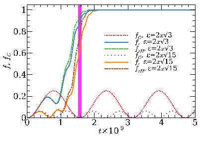
Our first study concerns the static detuning of the oracle Hamiltonian, i.e. when $\varepsilon$ has some fixed unknown value. It has been shown that stopping the evolution after the Grover time $T_{0}$ completely fails if the error parameter satisfies a “resonance condition” $\varepsilon=\pm 2x\sqrt{4m^{2}-1},$ for integer $m$ Novo et al. 2018, and behaves unfavourably in the neighbourhoods of these points. We carried out numerical simulations of both the original and the nonunitary search algorithm with parameters corresponding to panel (b) in Fig. 7 and using two different values of $\varepsilon$ satisfying the “resonance condition:” $\varepsilon=2x\sqrt{3}$ and $\varepsilon=2x\sqrt{15}$. For comparison, in Fig. 9 we have plotted the fidelity given by the original search Hamiltonian ($f_{G}$), the target fidelity of our nonunitary algorithm ($f$), as well as the target fidelity $f_{\mathrm{eff}}$ given by the approximate effective non-hermitian Hamiltonian description. The latter case corresponds to extending the Hamiltonian in Eq. (12) by an additional term corresponding to the oracle error: $H_{\mathrm{eff}}(t)\rightarrow H_{\mathrm{eff}}(t)-\varepsilon\ket{w}\bra{w}$. The thick vertical line in Fig. 9 indicates the readout step $n_{G}$ chosen obliviously to the error parameter $\varepsilon$. We have $P(n_{G})\approx 0.08$, $f(n_{G})\approx 0.88$ for $m=1$, and $P(n_{G})\approx 0.018$, $f(n_{G})\approx 0.63$ for $m=2$.

In order to compare the performance of our nonunitary protocol with continuous Grover search, let us introduce the “quality factor” $Q=f(n_{G})P(n_{G})/f_{G}(\pi/2x)$. As can be seen, $Q>1$ ($Q<1$) corresponds to the case when our proposed nonunitary algorithm is better (worse) than the standard Grover algorithm (we assume that measurements are instantaneous). In Fig. 10 we show the dependence of $Q$ as a function of the systematic oracle error $\varepsilon$. As can be seen, there is a set of intervals of $\varepsilon$ values where our nonunitary algorithm fares clearly better than the standard continuous search algorithm.

Now we turn to the analysis of the time-dependent detuning of the oracle, or a noisy driving of the Hamiltonian. In particular instead of Eq. (3) we consider the following Hamiltonian

where the noise function $f(t)$ has a mean value of $\overline{f(t)}=1$. Our numerical results for the $Q$ value are displayed in Fig. 11 we plot the $Q$ value for the case of noisy control with $f(t)$ modeled as a biased white noise (see inset of Fig. 11). As can be seen, the improvement in robustness is similar to that of constant detuning, shown in Fig. 10.

While our algorithm resembles the standard quantum Zeno-effect in that frequent measurements are carried out on the dynamical system and the continuation of the evolution is conditioned upon a correct measurement outcome Facchi and Pascazio 2008b, there are significant differences. The quantum Zeno effect can be observed when the survival probability at each measurement can be engineered to be arbitrarily close to unity, yielding a process that shares many features with adiabatic processes Burgarth et al. 2019. As a consequence, given a unitary evolution and projective measurements, the resulting Zeno dynamics in a restricted subspace becomes unitary as well. The quantum Zeno effect in quantum computing has found applications such as error correction Paz-Silva et al. 2012 and algorithm design Rudolph and Grover 2002; Hosten et al. 2006; Lin and Lin 2015. Common to these algorithmic applications is that the database registers are measured to induce the Zeno dynamics, while our algorithm uses measurements of the ancilla only. The quantum circuits studied in Refs. Rudolph and Grover 2002; Lin and Lin 2015 operate in the regime where the survival probability at each iteration is kept arbitrarily close to unity, thereby operating in the standard quantum Zeno regime.

The notion of bomb query complexity introduced by Lin et al. Lin and Lin 2015 showed a remarkable relation between Zeno dynamics and quantum query complexity, namely that the former is quadratically worse than the latter. However, since observation can lead to more complex dynamics Burgarth et al. 2014, this result appears to be specific to the simple measurement scheme and coupling between the ancilla and the oracle operation. As an example, we have shown here that our algorithm can retain the scaling of the quantum search algorithm.

Closest in spirit to our algorithm is the reported quantum search algorithm based on counterfactual quantum computing Hosten et al. 2006. Both approaches start with less than 1 survival probabilities in the initial iterations and quickly converge to a regime where the required measurement outcome is obtained with almost certainty, while exhibiting robustness against certain errors. The counterfactual search, however, suffers from a conceptual Mitchison and Jozsa 2006 and several technical drawbacks that our approach avoids. Namely, it requires the implementation of both the oracle and its adjoint, and it might be strongly affected by systematic errors in the oracle. In addition, no scalable analysis is presented in the paper, therefore it is not clear how the non-unit survival probability scales with the database size.

Finally, while the algorithm combining adiabatic quantum search by measurement employs a rather similar idea of coupling to an ancilla Childs et al. 2002, it uses a term $H_{o}\otimes p$ which is physically very non-trivial. In contrast, our coupling term is completely oblivious to the marked node.

In the case without detuning of the oracle, both the success probability of each step and the target fidelity are approaching 1 (see solid lines in Fig.7 and Fig.8). The saturation of the success probability makes the algorithm ideal for applications where verification queries to the classical database are impossible or come at a high cost. While the algorithm carries strong similarities with the quantum Zeno effect Misra and Sudarshan 1977; Exner 1985, and is based on the approach and techniques of Zeno-like dynamics in specific physical systems Nakazato et al. 2003; Li et al. 2011; Pyshkin et al. 2021 it employs a time-dependent sequence of projections (via parameter $\theta_{n}$). The protocol therefore shows similarities also with the proposal of von Neumann to transform quantum states by measurement von Neumann 1955, but in our protocol the final state is selected by the oracle Hamiltonian.

The synergy of quantum and classical computation in our algorithm is the result of selective measurements of the ancilla. The classical contribution in the efficiency $Q$ defined above is determined by the probability $P\leq 1$ (in pure quantum case $P=1$). The quantum/classical ratio of the algorithm can be tuned by properly choosing time intervals $\delta t$ between subsequent measurements. We note that our algorithm involves only a single quantum process, differing from studies considering the combined application of quantum and classical computers Bravyi et al. 2016.

In summary, we have presented a resource-efficient and robust nonunitary modification of the continuous version of Grover’s search based on measurements and conditional evolution. We have shown that this dynamics can be accurately described by a non-hermitian effective Hamiltonian in the Hilbert space $\mathcal{H}_{N}$, and determined its scaling properties under ideal conditions.

There are many possible directions for further development of similar protocols. For instance, the driven part of Hamiltonian, the parameters $\delta t$ and $\delta\theta$ can be made time-dependent (see e.g. Wilczek et al. 2020). We believe that the presented protocol will serve for a better understanding of controllable nonunitary processes and their scaling properties.

P. V. P. and A. G. are supported by the National Research, Development and Innovation Office of Hungary (NKFIH) Project No. K124351; P. V. P. by NKFIH through the Projects No. K115624, No. PD120975, No. 2017-1.2.1-NKP-2017-00001; and A. G. by MŠMT RVO 14000. P. V. P. and L. A. W. are supported by Grant No. PGC2018-101355-B-I00 funded by MCIN/AEI/10.13039/501100011033 and by “ERDF A way of making Europe”. L. A. W. is supported by the Grant No. PID2021-126273NB-I00 funded by MCIN/AEI/10.13039/501100011033, and the Basque Government through Grant No. IT1470-22. J. Q. Y. is supported by the National Natural Science Foundation of China (Grant No. 11934010). P. V. P. thanks Olga Masko for her support.

*

References

- Facchi and Pascazio (2008a) P. Facchi and S. Pascazio, Quantum zeno dynamics: mathematical and physical aspects, Journal of Physics A: Mathematical and Theoretical 41, 493001 (2008a).
- Rudolph and Grover (2002) T. Rudolph and L. Grover, Quantum searching a classical database (or how we learned to stop worrying and love the bomb), ArXiv quant-ph/0206066v (2002).
- Childs et al. (2002) A. M. Childs, E. Deotto, E. Farhi, J. Goldstone, S. Gutmann, and A. J. Landahl, Quantum search by measurement, Phys. Rev. A 66, 032314 (2002).
- Hosten et al. (2006) O. Hosten, M. T. Rakher, J. T. Barreiro, N. A. Peters, and P. G. Kwiat, Counterfactual quantum computation through quantum interrogation, Nature 439, 949 (2006).
- Lin and Lin (2015) C. Y.-Y. Lin and H.-H. Lin, Upper Bounds on Quantum Query Complexity Inspired by the Elitzur-Vaidman Bomb Tester, in 30th Conference on Computational Complexity (CCC 2015), Leibniz International Proceedings in Informatics (LIPIcs), Vol. 33, edited by D. Zuckerman (Schloss Dagstuhl–Leibniz-Zentrum fuer Informatik, Dagstuhl, Germany, 2015) pp. 537–566.
- Gilyén et al. (2019) A. Gilyén, Y. Su, G. H. Low, and N. Wiebe, Quantum singular value transformation and beyond: Exponential improvements for quantum matrix arithmetics, in Proceedings of the 51st Annual ACM SIGACT Symposium on Theory of Computing, STOC 2019 (Association for Computing Machinery, Phoenix, AZ, USA, 2019) pp. 193–204.
- Knill et al. (2001) E. Knill, R. Laflamme, and G. J. Milburn, A scheme for efficient quantum computation with linear optics, Nature 409, 46 (2001).
- Terashima and Ueda (2005) H. Terashima and M. Ueda, Nonunitary quantum circuit, International Journal of Quantum Information 03, 633 (2005).
- Kendon and Sanders (2005) V. Kendon and B. C. Sanders, Complementarity and quantum walks, Phys. Rev. A 71, 022307 (2005).
- Kendon and Maloyer (2008) V. Kendon and O. Maloyer, Optimal computation with non-unitary quantum walks, Theoretical Computer Science 394, 187 (2008), from Gödel to Einstein: Computability between Logic and Physics.
- Usher et al. (2017) N. Usher, M. J. Hoban, and D. E. Browne, Nonunitary quantum computation in the ground space of local hamiltonians, Phys. Rev. A 96, 032321 (2017).
- Nakazato et al. (2003) H. Nakazato, T. Takazawa, and K. Yuasa, Purification through zeno-like measurements, Phys. Rev. Lett. 90, 060401 (2003).
- Wu et al. (2004) L.-A. Wu, D. A. Lidar, and S. Schneider, Long-range entanglement generation via frequent measurements, Phys. Rev. A 70, 032322 (2004).
- Li et al. (2011) Y. Li, L.-A. Wu, Y.-D. Wang, and L.-P. Yang, Nondeterministic ultrafast ground-state cooling of a mechanical resonator, Phys. Rev. B 84, 094502 (2011).
- Pyshkin et al. (2016) P. V. Pyshkin, D.-W. Luo, J. Q. You, and L.-A. Wu, Ground-state cooling of quantum systems via a one-shot measurement, Phys. Rev. A 93, 032120 (2016).
- Pyshkin et al. (2021) P. V. Pyshkin, E. Y. Sherman, and L.-A. Wu, Polaron formation in a spin chain by measurement-induced imaginary zeeman field, Phys. Rev. B 104, 075136 (2021).
- Luchnikov and Filippov (2017) I. A. Luchnikov and S. N. Filippov, Quantum evolution in the stroboscopic limit of repeated measurements, Phys. Rev. A 95, 022113 (2017).
- Streltsov et al. (2011) A. Streltsov, H. Kampermann, and D. Bruß, Linking quantum discord to entanglement in a measurement, Phys. Rev. Lett. 106, 160401 (2011).
- Gilyén et al. (2015) A. Gilyén, T. Kiss, and I. Jex, Exponential sensitivity and its cost in quantum physics, Sci. Rep. 6, 20076 (2015).
- Coles and Piani (2014) P. J. Coles and M. Piani, Complementary sequential measurements generate entanglement, Phys. Rev. A 89, 010302(R) (2014).
- Torres et al. (2017) J. M. Torres, J. Z. Bernád, G. Alber, O. Kálmán, and T. Kiss, Measurement-induced chaos and quantum state discrimination in an iterated tavis-cummings scheme, Phys. Rev. A 95, 023828 (2017).
- Pyshkin et al. (2017) P. V. Pyshkin, D.-W. Luo, J. Q. You, and L.-A. Wu, Nondeterministic quantum computation via ground state cooling and ultrafast Grover algorithm, ArXiv (2017), arXiv:1704.01467 .
- Grimaudo et al. (2020) R. Grimaudo, A. Messina, A. Sergi, N. V. Vitanov, and S. N. Filippov, Two-qubit entanglement generation through non-hermitian hamiltonians induced by repeated measurements on an ancilla, Entropy 22, 1184 (2020).
- Amin et al. (2008) M. H. S. Amin, P. J. Love, and C. J. S. Truncik, Thermally assisted adiabatic quantum computation, Phys. Rev. Lett. 100, 060503 (2008).
- Luo et al. (2015) D.-W. Luo, P. V. Pyshkin, C.-H. Lam, T. Yu, H.-Q. Lin, J. Q. You, and L.-A. Wu, Dynamical invariants in a non-markovian quantum-state-diffusion equation, Phys. Rev. A 92, 062127 (2015).
- Novo et al. (2018) L. Novo, S. Chakraborty, M. Mohseni, and Y. Omar, Environment-assisted analog quantum search, Phys. Rev. A 98, 022316 (2018).
- Farhi and Gutmann (1998) E. Farhi and S. Gutmann, Analog analogue of a digital quantum computation, Phys. Rev. A 57, 2403 (1998).
- Wu and Byrd (2008) L.-A. Wu and M. S. Byrd, Self-protected quantum algorithms based on quantum state tomography, Quantum Information Processing 8, 1 (2008).
- Lidar and Wu (2003) D. A. Lidar and L.-A. Wu, Encoded recoupling and decoupling: An alternative to quantum error-correcting codes applied to trapped-ion quantum computation, Phys. Rev. A 67, 032313 (2003).
- Farhi et al. (2000) E. Farhi, J. Goldstone, S. Gutmann, and M. Sipser, Quantum Computation by Adiabatic Evolution, eprint arXiv:quant-ph/0001106 (2000), quant-ph/0001106 .
- Roland and Cerf (2002) J. Roland and N. J. Cerf, Quantum search by local adiabatic evolution, Phys. Rev. A 65, 042308 (2002).
- Pérez and Romanelli (2007) A. Pérez and A. Romanelli, Nonadiabatic quantum search algorithms, Phys. Rev. A 76, 052318 (2007).
- Li et al. (2018) F.-G. Li, W.-S. Bao, T. Li, H. liang Huang, S. Zhang, and X.-Q. Fu, Nonadiabatic quantum search algorithm with analytical success rate, International Journal of Theoretical Physics 58, 939 (2018).
- Salerno (1995) M. Salerno, The hubbard model on a complete graph: exact analytical results, Zeitschrift für Physik B Condensed Matter 99, 469 (1995).
- Jacko et al. (2017) A. C. Jacko, A. L. Khosla, J. Merino, and B. J. Powell, Spin-orbit coupling in , Phys. Rev. B 95, 155120 (2017).
- Lloyd (1996) S. Lloyd, Universal quantum simulators, Science 273, 1073 (1996).
- Wu et al. (2002) L.-A. Wu, M. S. Byrd, and D. A. Lidar, Polynomial-time simulation of pairing models on a quantum computer, Physical Review Letters 89, 057904 (2002).
- Smith et al. (2019) A. Smith, M. S. Kim, F. Pollmann, and J. Knolle, Simulating quantum many-body dynamics on a current digital quantum computer, npj Quantum Information 5, 106 (2019).
- Tacchino et al. (2020) F. Tacchino, A. Chiesa, S. Carretta, and D. Gerace, Quantum computers as universal quantum simulators: State‐of‐the‐art and perspectives, Advanced Quantum Technologies 3, 1900052 (2020).
- Shenvi et al. (2003) N. Shenvi, K. R. Brown, and K. B. Whaley, Effects of a random noisy oracle on search algorithm complexity, Phys. Rev. A 68, 052313 (2003).
- Facchi and Pascazio (2008b) P. Facchi and S. Pascazio, Quantum Zeno dynamics: Mathematical and physical aspects, J. Phys. A: Math. Theor. 41, 493001 (2008b).
- Burgarth et al. (2019) D. Burgarth, P. Facchi, H. Nakazato, S. Pascazio, and K. Yuasa, Generalized Adiabatic Theorem and Strong-Coupling Limits, Quantum 3, 152 (2019).
- Paz-Silva et al. (2012) G. A. Paz-Silva, A. T. Rezakhani, J. M. Dominy, and D. A. Lidar, Zeno Effect for Quantum Computation and Control, Phys. Rev. Lett. 108, 080501 (2012).
- Burgarth et al. (2014) D. K. Burgarth, P. Facchi, V. Giovannetti, H. Nakazato, S. Pascazio, and K. Yuasa, Exponential rise of dynamical complexity in quantum computing through projections, Nat Commun 5, 5173 (2014).
- Mitchison and Jozsa (2006) G. Mitchison and R. Jozsa, The limits of counterfactual computation, ArXiv quant-ph/0606092v3 (2006).
- Misra and Sudarshan (1977) B. Misra and E. C. G. Sudarshan, The Zeno’s paradox in quantum theory, Journal of Mathematical Physics 18, 756 (1977).
- Exner (1985) P. Exner, Open Quantum Systems and Feynman Integrals, Fundamental Theories of Physics (Springer Netherlands, 1985).
- von Neumann (1955) J. von Neumann, Mathematical Foundations of Quantum Mechanics (Princeton Univ Press, Princeton, 1955) pp. 365–367.
- Bravyi et al. (2016) S. Bravyi, G. Smith, and J. A. Smolin, Trading classical and quantum computational resources, Phys. Rev. X 6, 021043 (2016).
- Wilczek et al. (2020) F. Wilczek, H.-Y. Hu, and B. Wu, Resonant quantum search with monitor qubits, Chinese Physics Letters 37, 050304 (2020).
- Dattoli et al. (1990) G. Dattoli, A. Torre, and R. Mignani, Non-hermitian evolution of two-level quantum systems, Phys. Rev. A 42, 1467 (1990).
- Bagchi (2018) B. Bagchi, Evolution operator for time-dependent non-hermitian hami ltonians, Letters in High Energy Physics 1, 4 (2018).