Quantum Sequential Hypothesis Testing
Abstract
We introduce sequential analysis in quantum information processing, by focusing on the fundamental task of quantum hypothesis testing. In particular our goal is to discriminate between two arbitrary quantum states with a prescribed error threshold, , when copies of the states can be required on demand. We obtain ultimate lower bounds on the average number of copies needed to accomplish the task. We give a block-sampling strategy that allows to achieve the lower bound for some classes of states. The bound is optimal in both the symmetric as well as the asymmetric setting in the sense that it requires the least mean number of copies out of all other procedures, including the ones that fix the number of copies ahead of time. For qubit states we derive explicit expressions for the minimum average number of copies and show that a sequential strategy based on fixed local measurements outperforms the best collective measurement on a predetermined number of copies. Whereas for general states the number of copies increases as , for pure states sequential strategies require a finite average number of samples even in the case of perfect discrimination, i.e., .
Introduction.
Statistical inference permeates almost every human endeavor, from science and engineering all the way through to economics, finance, and medicine. The perennial dictum in such inference tasks has been to optimize performance—often quantified by suitable cost functions—given a fixed number, , of relevant resources Lehmann and Casella 2006; Helstrom 1976. This approach often entails the practical drawback that all resources need to be batch-processed before a good inference can be made. Fixing the number of resources ahead of time does not reflect the situation that one encounters in many real-life applications that might require an online, early, inference–such as change-point detection Tartakovsky et al. 2014; Sentís et al. 2016; Sentís et al. 2017; Sentís et al. 2018, or where additional data may be obtained on demand if the required performance thresholds are not met.
Sequential analysis Wald 1973 is a statistical inference framework designed to address these shortcomings. Resources are processed on-the-fly, and with each new measured unit a decision to stop the experiment is made depending on whether prescribed tolerable error rates (or other cost functions) are met; the processing is continued otherwise. Since the decision to stop is solely based on previous measurement outcomes, the size of the experiment is not predetermined but is, instead, a random variable. A sequential protocol is deemed optimal if it requires the least average number of resources among all statistical tests that guarantee the same performance thresholds. For many classical statistical inference tasks it is known that sequential methods can attain the required thresholds with substantially lower average number of samples than any statistical test based on a predetermined number of samples Wald 1973. The ensuing savings in resources, and the ability to take actions in real-time, have found applications in a wide range of fields Leung Lai 2001; Tartakovsky et al. 2014. Extending sequential analysis to the quantum setting is of fundamental interest, and with near-term quantum technologies on the verge of impacting the global market, the versatility and resource efficiency that sequential protocols provide for quantum information processing is highly desirable.
In this paper we consider the discrimination of two arbitrary finite dimensional quantum states Bae and Kwek 2015, (corresponding to the null hypothesis ) and (corresponding to the alternative hypothesis ), in a setting where a large number of copies can be used in order to meet a desired error threshold . A first step in this direction was taken in Ref. Slussarenko et al. 2017, which considers the particular case where and are pure states and restricts the analysis to specific local measurement strategies. Here, we address the problem in full generality, including arbitrary states, weak and collective measurements. For collective strategies involving a large fixed number of copies the relation between this number and the error is 11 1 By we mean asymptotic equivalence , where the rate depends on the pair of hypotheses and on the precise setting as we explain shortly. We show that one can significantly reduce the expected number of copies, , by considering sequential strategies where copies are provided on demand. We give the ultimate lower-bounds as a single-letter expression of the form,
| (1) |
for , where is the mean number of copies given the true hypothesis is and is the quantum relative entropy. In addition, we provide upper bounds which, for the worst case , are achievable for some families of states.
Specifically, we consider quantum hypothesis testing in a scenario where one can guarantee that for each realization of the test the conditional probability of correctly identifying each of the hypotheses is above a given threshold. This scenario, first introduced in Slussarenko et al. 2017, can be considered genuinely sequential since such strong error conditions cannot be generally met in a deterministic setting. The proof method can be easily extended to the more common asymptotic symmetric and asymmetric scenarios involving the usual type I (or false positive) and type II (or false negative) errors. We give the optimal scaling of the mean number of copies when the thresholds for either one or both types of errors are asymptotically small.
Before proceeding, let us briefly review these fundamental hypothesis testing scenarios, which come about from the relative importance one places between type I error—the error of guessing the state to be when the true state is whose probability we denote by —and type II error—the error of guessing when the state is whose probability is . Often, the two types of errors are put on equal footing (symmetric scenario) and one seeks to minimise the mean probability of error with the prior probabilities for each hypothesis. The mean error decays exponentially with the number of copies with an optimal rate given by the Chernoff distance Audenaert et al. 2007; Nussbaum and Szkoła 2009, .
Yet, there are asymmetric instances, e.g., in medical trials, where the effect of approving an ineffective treatment (type-II) is far worse than discarding a potentially good one (type-I). In such cases it is imperative to minimise the type II error whilst maintaining a finite probability of successfully identifying the null hypothesis, i.e., . The corresponding optimal error rate for quantum hypotheses is given by quantum Stein’s lemma Hiai and Petz 1991; Ogawa and Nagaoka 2000, where is the quantum relative entropy. If, on the other hand, we require the type I error to decay exponentially, i.e., for some rate , then the optimal rate is given by the quantum Hoeffding bound Hayashi 2007; Nagaoka 2006. These optimal error rates for strategies with fixed number of copies have found applications in quantum Shannon theory Wilde 2017, quantum illumination Lloyd 2008, and provide operational meaning to abstract information measures Audenaert et al. 2008; Calsamiglia et al. 2008; Berta et al. 2017.
What the above results also show is that for fixed there is a trade-off between the probabilities of committing either error. The advantage of sequential analysis is that it provides strategies capable of minimising the average number of copies when both errors are bounded, and yields higher asymptotic rates in each of the settings described above.
Fixed local measurements.
We begin by considering the case when each quantum system is measured with the same measurement apparatus , giving rise to identically distributed samples of a classical probability distribution. This strategy has the advantage of being easily implementable, and that it lets us introduce the classical sequential analysis framework. Specifically, the optimal classical sequential test, for both the strong error as well as the symmetric and asymmetric setting, is known to be the Sequential Probability Ratio Test (SPRT)Wald and Wolfowitz 1948 which we now review.
After measurements have been performed, we have a string of outcomes , where each element has been sampled effectively from a probability distribution determined by the POVM and the true state of the system, i.e., either , or . For given error thresholds , the strong condition demands that for each conclusive sequence the conditional probabilities obey either
| (2) | ||||
| (3) |
where since the copies are identical and independent (the same holds for ). If neither condition is met, a new copy needs to be requested and we continue measuring. That is, starting at at every step we check whether
- 1.
, then STOP and accept , with guaranteed probability of success .
- 2.
, then STOP and accept , with guaranteed probability of success .
- 3.
If neither 1 nor 2 hold, continue sampling.
Using (2) and (3), the condition to continue sampling can be written in terms of a single sample statistic, the log-likelihood ratio
| (4) |
as , where , .

It is convenient to interpret as a random walk (see Fig. 1) that at every instance performs a step of length with probability , if holds, or with probability , if holds. Under the mean position of the walker at step is given by where is the relative entropy; while for , . That is, under the walker has a drift towards the positive axis, while under it drifts towards the negative axis. We define as the stopping time the first instance in which the walker steps out of the region , i.e., , and note that it is a stochastic variable that only depends on the current as well as the past measurement record. The stochastic variable is the position of the walker at . The mean value of this position can be related to the mean number of steps by Wald’s identity Mitzenmacher and Upfal 2005,
| (5) |
under hypothesis , and likewise . In order to estimate from (5) we need to provide a good estimate for . For this purpose let us first define as the set of strings such that for all and , and as the set of strings such that for all and . Then, the following relations hold:
| (6) | ||||
where in the first (second) inequality we used that for strings in ( for strings in ), and in the last equality we have used that Wald and Wolfowitz 1948, i.e. the walker eventually stops. The above equations are an instance of so-called Wald’s likelihood ratio identity Lai 2004. We note that the above inequalities can be taken to be approximate equalities if we assume that the process ends close to the prescribed boundary, i.e. there is no overshooting. In particular, this will be valid in our asymptotically small error settings where the boundaries are far relative to the (finite) step size . This allows us to establish a one-to-one correspondence between the thresholds and the type I & II errors: and . Gendra et al. 2012; Audenaert and Eisert 2005 Neglecting the overshooting also allows us to consider as a stochastic variable that takes two values . Under hypothesis , occurs with probability and with ; while under hypothesis , and occur with probabilities and . So,
| (7) |
Making use of (5) one can now write a closed expression for and in terms of and the priors. A remarkable property of the SPRT with error probabilities and is that it minimizes both and among all tests (sequential or otherwise) with bounded type I and type II errors. This optimality result due to Wald and Wolfowitz Wald and Wolfowitz 1948 allows us to extend the above results to the asymmetric scenario. For the symmetric scenario, the SPRT has also been shown Simons 1976 to be optimal among all tests respecting a bounded mean error . In the asymptotic limit of small error bounds, , the threshold values are and , which correspond to and , yielding
| (8) |
The same expressions hold at leading order in the asymmetric scenario when the type I & II errors are vanishingly small, replacing and by and respectively—and in the symmetric scenario replacing both quantities by . If one of the error thresholds, say , is kept finite while the second is made vanishingly small , remains finite, while the other conditional mean scales as .
In the supplemental material SM we apply these results to the discrimination of qubit states using projective measurements and give closed expressions for the optimal Bayesian mean number of copies . Figure 2 shows that in the symmetric setting these restricted sequential strategies already require on average between 25-50% less resources than the best deterministic strategy that uses a fixed number of copies Calsamiglia et al. 2008; Audenaert et al. 2007, and requires non-trivial collective measurements Calsamiglia et al. 2010.

Ultimate quantum limit.
Quantum mechanics allows for much more sophisticated strategies. For a start, performing a non-projective generalized measurement already gives important advantages (see below). One can also adapt the measurements depending on the previous measurement outcomes and, importantly, measurements may be weak so that each new measurement acts on a fresh copy but also on the preceding, already measured, copies. Without loss of generality we can assume that at every step we perform a measurement with three outcomes : the first two must fulfill conditions (2) and (3) and trigger the corresponding guess ( or respectively), while the third outcome signals to continue measuring having an additional fresh copy available. The measurement at step is characterized by a quantum instrument , and the sequential strategy is given by a sequence of instruments . With this, given hypothesis , the probability of getting outcome at step can be written as
| (9) |
where we have used that in order to arrive to step a “continue” outcome must be triggered in all previous steps, and in the last equality we have defined the effective POVM . Making use of the indicator function , the mean number of steps under hypothesis can be computed as
| (10) |
where is the probability that the sequence does not stop at step , which from (9) is given by . Optimizing over all quantum sequential strategies is daunting, as all terms are strongly interrelated through the intricate structure of . However, a lower bound to each can be found by relaxing such structure and only imposing minimal requirements on the effective POVM; namely the error bounds (6), positivity and completeness:
| (11) | ||||
This semi-definite program, which can be considered a two-sided version of the quantum Neyman-Pearson test Audenaert et al. 2008, is an interesting open problem in its own right. Our focus, however, is the asymptotic regime of small error bounds. In these asymptotic scenarios we are able to show, exploiting some recent strong converse results in hypothesis testing Cooney et al. 2016; Beigi et al. 2020, that for all , for some SM, which leads to the desired bound:
| (12) |
An analogous bound holds for . The bounds for asymmetric (symmetric) scenarios (see SM) take the same form, replacing by () and by (). In the asymmetric scenario where or is kept finite, it also holds that and is given by the appropriate version of (12).
Attainability and upper bounds.
Consider a sequential strategy that involves a fixed, collective measurement , acting on consecutive blocks of copies, yielding two possible distributions . Using the classical SPRT we get that
| (13) |
where is the number of blocks used at the stopping time. In the last relation of (13) we have used the fact that we are in the asymptotic setting where and therefore we can take arbitrarily long block lengths . We also exploit the following property of the measured relative entropy Hiai and Petz 1991; Hayashi 2001: .
Notice, however, that for arbitrary states and block sampling can attain either or , but it is unknown whether one can attain in general both bounds simultaneously, i.e., whether a measurement achieving the supremum of can also attain the supremum of . For instance, if we wish to optimize the Bayesian mean number of copies , we can use block sampling to attain
| (14) |
However, this strategy might be sub-optimal and hence it only provides an upper bound to the optimal Bayesian mean . This notwithstanding, there are at least two cases when this upper bound coincides with the lower bound provided by (12): when and commute, and when the two states do not have common support. If, say, , one can use block-sampling to attain (12) for and always detect with a finite number of copies—note that since , the lower bound is also attained.
We can also give achievable lower bounds for a worst-case type figure of merit . If, say, , then in SM we give some instances of qubit pairs where a specific block-sampling strategy Hayashi 2001 saturates (12) for , while at the same time , and hence (12) provides the ultimate attainable limit for . In Fig. 2 we compare with for several pairs of states, highlighting the achievable cases, and show a consistent advantage of sequential protocols over deterministic ones 22 2 Note that the comparison with is unfavorable to sequential strategies. Substituting and by in Eq. (12) implies that each type of error is independently constrained, whereas refers to a deterministic (symmetric) protocol where the mean error is and thus to a weaker version of the problem. In spite of this, the sequential scenario displays a significant advantage..
Finally, we note that, in an asymmetric scenario where is finite and the value of achieves the lower bound (12), sequential protocols provide a strict advantage over Stein’s limit for deterministic protocols by a factor .
The curious case of pure states.
If the two states are pure, the behavior of changes drastically: it is possible to reach a decision with guaranteed zero error using a finite average number of copies. To see this, consider again Eq. (18). Under a zero-error condition, the minimal (unrestricted) is achieved by a global unambiguous three-outcome POVM Ivanovic 1987; Dieks 1988; Peres 1988 on copies, which identifies the true state with zero error when the first or the second outcome occurs —at the expense of having a third, inconclusive outcome. For a single-copy POVM over pure states, the probabilities of the inconclusive outcome under are subject to the tradeoff relation Sentís et al. 2018, where equality can always be attained by suitable POVM that maximizes the probability of a successful identification. Likewise, for a global measurement on copies we have . Now, it is evident that a sequence of locally optimal unambiguous POVMs applied on every copy, for which , also fulfills the global optimality condition. Hence, we have
| (15) |
This shows that, for pure states, it suffices to perform local unambiguous measurements to attain the optimal (finite) average number of copies with zero error under hypothesis . Note that because of the tradeoff one cannot attain the minimal values of and for general states , simultaneously. For instance, one can reach the minimal value for one hypothesis, but then having a maximal value for the second; or choose the optimal symmetric setting, , that achieves the minimum value of both the worst-case and the Bayesian mean with equal priors (see SM). This is in stark contrast with the behavior found in Slussarenko et al. 2017, where all strategies considered were based on two-outcome projective measurements, for which the average number of copies scaled as .
Acknowledgments.
We acknowledge financial support from the Spanish Agencia Estatal de Investigación, project PID2019-107609GB-I00, from Secretaria d’Universitats i Recerca del Departament d’Empresa i Coneixement de la Generalitat de Catalunya, co-funded by the European Union Regional Development Fund within the ERDF Operational Program of Catalunya (project QuantumCat, ref. 001-P-001644), and Generalitat de Catalunya CIRIT 2017-SGR-1127. CH acknowledge financial support from the European Research Council (ERC Grant Agreement No. 81876), VILLUM FONDEN via the QMATH Centre of Excellence (Grant No.10059) and the QuantERA ERA-NET Cofund in Quantum Technologies implemented within the European Union Horizon 2020 Programme (QuantAlgo project) via Innovation Fund Denmark, JC acknowledges from the QuantERA grant C’MON-QSENS!, via Spanish MICINN PCI2019-111869-2, EMV thanks financial support from CONACYT. JC also acknowledges support from ICREA Academia award.
References
- Lehmann and Casella (2006) E. L. Lehmann and G. Casella, Theory of point estimation, 2nd ed. (Springer Science & Business Media, 2006).
- Helstrom (1976) C. W. Helstrom, Quantum Detection and Estimation Theory (Academic Press, 1976).
- Tartakovsky et al. (2014) A. G. Tartakovsky, I. V. Nikiforov, and M. Basseville, Sequential Analysis: hypothesis testing and changepoint detection, edited by F. Bunea, V. Isham, N. Keiding, T. Louis, R. L. Smith, and H. Tong (CRC Press, Taylor and Francis, 2014).
- Sentís et al. (2016) G. Sentís, E. Bagan, J. Calsamiglia, G. Chiribella, and R. Muñoz Tapia, Phys. Rev. Lett. 117, 150502 (2016).
- Sentís et al. (2017) G. Sentís, J. Calsamiglia, and R. Muñoz Tapia, Phys. Rev. Lett. 119, 140506 (2017).
- Sentís et al. (2018) G. Sentís, E. Martínez-Vargas, and R. Muñoz Tapia, Phys. Rev. A 98, 052305 (2018).
- Wald (1973) A. Wald, Sequential Analysis, Dover books on advanced mathematics (Dover Publications, 1973).
- Leung Lai (2001) T. Leung Lai, Statistica Sinica 11, 303 (2001).
- Bae and Kwek (2015) J. Bae and L.-C. Kwek, Journal of Physics A: Mathematical and Theoretical 48, 083001 (2015).
- Slussarenko et al. (2017) S. Slussarenko, M. M. Weston, J.-G. Li, N. Campbell, H. M. Wiseman, and G. J. Pryde, Physical Review Letters 118, 030502 (2017).
- (11) By we mean asymptotic equivalence .
- Audenaert et al. (2007) K. M. R. Audenaert, J. Calsamiglia, R. Muñoz-Tapia, E. Bagan, L. Masanes, A. Acín, and F. Verstraete, Physical Review Letters 98, 160501 (2007).
- Nussbaum and Szkoła (2009) M. Nussbaum and A. Szkoła, Annals of Statistics 37, 1040 (2009).
- Hiai and Petz (1991) F. Hiai and D. Petz, Communications in Mathematical Physics 143, 99 (1991).
- Ogawa and Nagaoka (2000) T. Ogawa and H. Nagaoka, IEEE Transactions on Information Theory 46, 2428 (2000).
- Hayashi (2007) M. Hayashi, Physical Review A 76, 062301 (2007).
- Nagaoka (2006) H. Nagaoka, arXiv:quant-ph/0611289 (2006).
- Wilde (2017) M. M. Wilde, Quantum Information Theory, 2nd ed. (Cambridge University Press, 2017).
- Lloyd (2008) S. Lloyd, Science 321, 1463 (2008).
- Audenaert et al. (2008) K. M. R. Audenaert, M. Nussbaum, A. Szkola, and F. Verstraete, Communications in Mathematical Physics 279, 251 (2008).
- Calsamiglia et al. (2008) J. Calsamiglia, R. Muñoz-Tapia, L. Masanes, A. Acin, and E. Bagan, Physical Review A 77, 032311 (2008).
- Berta et al. (2017) M. Berta, F. G. Brandao, and C. Hirche, arXiv:1709.07268 (2017).
- Wald and Wolfowitz (1948) A. Wald and J. Wolfowitz, The Annals of Mathematical Statistics 19, 326 (1948).
- Mitzenmacher and Upfal (2005) M. Mitzenmacher and E. Upfal, Probability and Computing: Randomized Algorithms and Probabilistic Analysis (Cambridge University Press, 2005).
- Lai (2004) T. L. Lai, Sequential Analysis 23, 467 (2004).
- Simons (1976) G. Simons, The Annals of Statistics 4, 1240 (1976).
- (27) See Supplemental Material [url] where we provide the proof of the lower bound for the mean number of copies under each hypothesis, we apply our general results to the case of qubit states, we compute the exact optimal mean number of copies (worst-case and Bayesian) required for the perfect discrimination of pure states, and which includes Mosonyi and Ogawa 2015; Müller-Lennert et al. 2013; Wilde et al. 2014; Beigi et al. 2020; Acín et al. 2005; Gendra et al. 2012; Audenaert and Eisert 2005.
- Mosonyi and Ogawa (2015) M. Mosonyi and T. Ogawa, Communications in Mathematical Physics 334, 1617 (2015).
- Müller-Lennert et al. (2013) M. Müller-Lennert, F. Dupuis, O. Szehr, S. Fehr, and M. Tomamichel, Journal of Mathematical Physics 54, 122203 (2013).
- Wilde et al. (2014) M. M. Wilde, A. Winter, and D. Yang, Communications in Mathematical Physics 331, 593 (2014).
- Beigi et al. (2020) S. Beigi, N. Datta, and C. Rouzé, Communications in Mathematical Physics 376, 753 (2020).
- Acín et al. (2005) A. Acín, E. Bagan, M. Baig, L. Masanes, and R. Muñoz-Tapia, Physical Review A 71, 032338 (2005).
- Gendra et al. (2012) B. Gendra, E. Ronco-Bonvehi, J. Calsamiglia, R. Muñoz-Tapia, and E. Bagan, New Journal of Physics 14, 105015 (2012).
- Audenaert and Eisert (2005) K. M. Audenaert and J. Eisert, Journal of Mathematical Physics 46, 102104 (2005).
- Calsamiglia et al. (2010) J. Calsamiglia, J. I. de Vicente, R. Muñoz-Tapia, and E. Bagan, Physical Review Letters 105, 080504 (2010).
- Cooney et al. (2016) T. Cooney, M. Mosonyi, and M. M. Wilde, Communications in Mathematical Physics 344, 797 (2016).
- Hayashi (2001) M. Hayashi, Journal of Physics A: Mathematical and General 34, 3413 (2001).
- (38) Note that the comparison with is unfavorable to sequential strategies. Substituting and by in Eq. (12) implies that each type of error is independently constrained, whereas refers to a deterministic (symmetric) protocol where the mean error is and thus to a weaker version of the problem. In spite of this, the sequential scenario displays a significant advantage.
- Ivanovic (1987) I. Ivanovic, Physics Letters A 123, 257 (1987).
- Dieks (1988) D. Dieks, Physics Letters A 126, 303 (1988).
- Peres (1988) A. Peres, Physics Letters A 128, 19 (1988).
I Supplemental Material
This supplemental material contains some technical details as well as some extensions for the interested reader. In Sec. II we state and prove a theorem that provides the lower bounds for the average number of copies, Eq. (12) in the main text. In Sec. III explicit expressions for the optimal sequential test and attainability regions of the worst case bound are provided for the qubit case. In Sec. IV we present a second theorem that provides a general lower bound for the deviation of the measured entropy from its maximum value for arbitrary finite dimensions. Finally, in Sec. V we give the optimality proof for the zero-error protocol for pure states.
II Converse proof
Our aim here is to prove that if one of the two error bounds is vanishingly small, say under the strong error condition, or in the asymmetric scenario (see main text for the definitions), then the mean number of copies under hypothesis is always lower-bounded by
| (16) | ||||
| (17) |
respectively. Analogous bounds also hold for when or , replacing , , , and . We will first provide the proof for the strong error condition and indicate how to adapt it to the other hypothesis testing scenarios considered here.
In the main text (MT) we have shown that under hypothesis the mean number of sampled copies is given by
| (18) |
where the last inequality holds for all values of since . The th term in sum, , is the probability of getting a “continue” outcome at step , corresponding to the POVM element implicitly defined in (12) in MT. The continue probability at a particular step obeys a lower bound given by the following semidefinite program (SDP)
| (19) |
The conditions in 0) have to hold for any valid POVM, while the second and third conditions are an alternative way of writing the strong errors conditions, (1) and (2) in the MT, as SDP constrains. For small error bounds (i.e. ) the solution of the SDP program in (19) has a characteristic dependence on as illustrated in Figure 3.
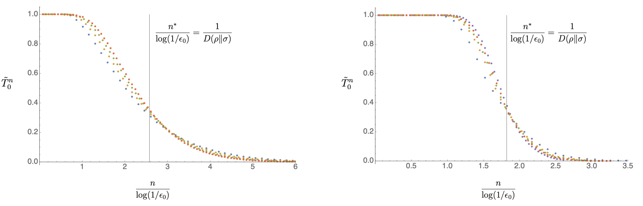
When the number of sampled copies is small it is not possible to meet the low error bound and the probability of getting a “continue” outcome is . This probability remains constant as increases until it approaches the critical point , at which point it rapidly drops to zero. Note that this drop becomes more abrupt as decreases. These observations suggest that is a very tight lower bound to (area under the curve in Figure 3) and is given to a very good approximation by .
With this at hand we can now carry on with the formal presentation and proof of the lower bound.
Theorem 1.
Given two finite-dimensional states, () and (), occurring with prior probabilities and respectively, the most general quantum sequential strategy that satisfies the strong error conditions and , where is the output of the measurement at the stopping time , necessarily fulfills the following asymptotic lower bound for the mean number of sampled copies when :
| (20) |
Similarly, the most general quantum sequential strategy that satisfies the (weak) error conditions and , where and are the events of accepting hypothesis 0 and 1 respectively, necessarily fulfills the following asymptotic lower bound for the mean number of sampled copies when :
| (21) |
Proof.
We start by noting that the strong error conditions [see (19)] imply
| (22) | |||||
| (23) |
Next we form a two-outcome POVM by binning two outcomes of the effective POVM at step , as defined in (12) in MT, . This measurement can be used to discriminate between and and the associated type-I and type-II errors will be denoted by and . From (23) and the above definitions it follows that . In addition, using (23) we find that the probability of continuing at step when holds satisfies
| (24) |
Now we use Lemma 1 stated below, which uses the recently developed methods for strong converse exponents Cooney et al. 2016 in order to establish a lower bound on when the type-II error is bounded by and when is below a critical threshold . In particular, applying Lemma 1 to the test defined by above, with type-I & II errors and , we have that (24) reads
| (25) |
where . The proof for the strong error conditions ends by inserting this lower bound in (18).
For the weak form of error bounds one can follow the same steps as above by writing the type-I and type-II errors of the sequential strategy as and . Since , the error bound translates to , and similarly . The former is directly of the form required for Lemma 1, while the latter can be used instead of (22), i.e., , hence in (20) becomes in (21).
∎
Lemma 1.
Let and be finite-dimensional density operators associated to hypotheses and , respectively. For any quantum hypothesis testing strategy that uses copies of the states and that respects the type-II error bound , with , the type-I error will converge to one at least as
| (26) |
where is given by
| (27) |
where is the strong converse exponent (Mosonyi and Ogawa 2015) and where the sandwiched Renyi relative entropy Müller-Lennert et al. 2013; Wilde et al. 2014 is given by
| (28) |
taking when .
Proof.
The proof makes use of the following strong converse result by Mosonyi and Ogawa Mosonyi and Ogawa 2015 that relates the type I and type II errors for an arbitary by means of the sandwiched Renyi relative entropy:
| (29) |
Note that in order to avoid confusion with the type-I error, here we use instead of the traditional used in the Renyi entropies. Among the number of properties that make the sandwiched Renyi relative entropy such a formidable quantity, here we will use two: i) it increases monotonically with , and ii) .
Since ,
| (30) |
Observe that we can define such that
| (31) |
Using this parametrization of in (30), we have
| (32) |
Hence, if we define the supremum of the exponent
| (33) |
we arrive to the desired result
| (34) |
Taking into account that for all , that for , and from conditions i) and ii) above that , it follows that there will always be an realizing the supremum in (33) such that , and therefore . ∎
An alternative way to arrive to the result in Lemma 1 is provided in Beigi et al. Beigi et al. 2020 where, using quantum reverse hypercontractivity, a second order strong converse result on hypothesis testing is derived.
We finally note that Lemma 1 assures that, below , the continue probability is . On the other hand, from Stein’s Lemma we know that, for fixed (large) , the optimal type-II error rate is given by the relative entropy, i.e., . This explains why one does not need to continue measuring after , and (see Fig. 3), and why we may expect the lower bound to be tight, in the sense that we are not dropping significant contributions by truncanting the sum in (18). Of course, this still does not imply the attainability of the lower bound, and even less the simultaneous attainability of the bound for and the analogous bound for .
III Sequential hypothesis testing for Qubits
In this section we study the discrimination of qubit states using sequential methodologies, deriving explicit formulae for the mean number of copies using different measurement strategies.
III.1 Optimal sequential test for fixed projective measurements
We will first study the optimal performance under the simplest type of measurement apparatus, i.e. a fixed Stern-Gerlach-type measurement. The main purpose of this section is to show that using sequential strategies a simple projective measurement can determine the correct hypothesis with guaranteed bounded error requiring an expected number of copies significantly lower than the most general collective measurement acting on a fixed number of copies. In addition, we provide closed expressions for the optimal asymptotic performance.
Without loss of generality we characterize the two hypotheses by
| (35) |
where , , and the (fixed) local measurement as and , with , and . With these parametrizations, the probabilities of obtaining outcome are and , depending on which hypothesis is true. For simplicity we take equal priors and study the Bayesian mean number of copies under the same strong error bounds . In the main text we show that the optimal test for a given choice of measurement angle is given by Wald’s SPRT strategy, which according to (11) in MT leads to
| (36) |

In Figure 4 we show the Bayesian mean number of copies required to have a guaranteed, asymptotically small bounded error for all outcomes of the experiment. For pure states (), we observe that the optimal angle is a singular point located at , that corresponds to the fully biased measurement for which outcome 1 can only occur under hypothesis while . Hence, is detected with certainty after a small number of steps (independent of the error bound ), and therefore the leading contribution to the expected number of copies when hypothesis is true is
| (37) |
Note that this is exactly half of the number of copies that the most general collective deterministic strategy would require to attain this error bound, since . This error bound can be attained with local adaptive measurements for finite Acín et al. 2005 and fixed local measurements for asymptotically large . The result in (37) is in agreement with that derived in Slussarenko et al. 2017 for the fully biased strategy, which we have shown to be optimal in the limit of small error bounds (among fixed local measurement strategies). In Figure 4 we also note that a small change around the optimal value produces a very rapid increase of the effective number of copies while the local minimum at , which corresponds to the fully unbiased measurement, is much more shallow and hence more robust to a possible measurement misalignment.
We now proceed to study what happens in the presence of noise, when both states are mixed, in particular when . As shown in the inset of Figure 4, the presence of noise makes the two states more indistinguishable and a higher number of samples are required to meet the error bound. It is also apparent that in presence of noise the fully unbiased measurement, , becomes optimal (except for extremely high values of the purity for which fully biased performs slightly better). The unbiased measurement is straightforward to compute:
| (38) |
We can again compare reached by the local measurements (38)with the sample size, , required by the optimal deterministic protocol using a predetermined number of copies to achieve the same error . When is large, i.e. is small, this can be obtained from the asymptotic error exponent in the quantum Chernoff bound Calsamiglia et al. 2008; Audenaert et al. 2007. We find
| (39) |
In Figure 2 in MT we compare Eqs. (38) and (39) and observe a reduction of the required number of copies of at least 50% on average if we employ the sequential test instead of the deterministic one. The reduction goes up to 75% if and are very mixed.

For illustration purposes, in Figure 5 we show explicitly the results of several runs of a SPRT using unbiased local measurements. We observe how the mean trajectories that the cummulative log-likelihood ratio follows point upwards or downwards depending on the underlying hypothesis. In this simulation, the state , corresponding to , is identified quicker than (the decision boundary is closer than ), despite being more mixed. A histogram of stopping times under each hypothesis shows us that the distributions of are well-centered around their empirical mean, with right tails that are slightly longer; this is also apparent on the left figure from the cross-sections of the trajectories with the decision boundaries. Finally, we observe that the mean number of copies increases linearly with for , as predicted.
III.2 Block-sampling and irrep projection
Here we study the mean number of copies under both hypotheses using a block-sampling strategy where the same collective measurement is repeated on batches of copies. In particular we will consider a collective measurement for which Hayashi Hayashi 2001 showed that the (classical) relative entropy of the distributions that arise from it, attains the quantum relative entropy when the block length is large. Denoting by such collective POVM and by the probability distributions of the outcomes, i.e., and , in Ref. Hayashi 2001 it is shown that
| (40) |
where is the dimension of the underlying Hilbert space, from where
| (41) |
Quite remarkably, the measurement in Eq. (40) depends solely on state .
As explained in the MT such a strategy allows one to attain the lower bound for one of the hypotheses, say for the strong error bounds [cf. Eq. (15) in MT], or
| (42) |
for the asymmetric setting.
In what follows we compute the (sub-optimal) performance of this very same measurement under the other hypothesis, i.e., .
For qubit systems, the POVM that achieves the quantum relative entropy Hayashi 2001 corresponds to the simultaneous measurement of the total angular momentum (eigenspaces labeled by ) and its component along the axis (eigenspaces labeled by ), where is picked to be the axis along which the state points, i.e., . The quantum number labels the irreducible representations (irreps), and since it is invariant under the action of any rigid rotation it will only provide information about the spectra of or —which we denote for respectively. The second measurement is clearly not invariant and provides information about relative angle between both hypotheses, and additional information on their spectrum.
Due to the permutational invariance of the copies it is possible to write the states in a block-diagonal form in terms of the quantum numbers (see e.g. Gendra et al. 2012):
| (43) |
where are projectors over the subspaces of dimension that host the irreps of the permutation group (i.e. multiplicity space of spin ), for even ( for odd) and
| (44) | |||||
| (45) |
are normalized probability distributions.
Under hypothesis the state has exactly the same structure except for a global rotation around the axis by an angle ,
| (46) |
where and take the form of (44) and (45) replacing and by and .
The outcomes of the and measurements lead to probability distributions
| (47) | ||||
| (48) |
whose relative entropy can be written as
| (49) |
where we have used the fact that for , is strongly peaked at and decays exponentially, and hence it is peaked at . In addition we note that
| (50) |
where we used the general decomposition of (46), and is short-hand notation for . Inserting this expression in (49) and using the definitions in (44) and (45) we finally arrive at
| (51) |
where the symbol recalls that we have chosen as a measurement over the eigenbasis of , which maximizes the relative entropy , and
| (52) |
is the relative entropy between the spectra of and . Hence, the second term in (51) can be associated to the distinguishability caused by the different orientation (non-commutativity) of the states.
On the other hand, from (41) it follows
| (53) |
From the above results we conclude that applying the measurement that reaches the ultimate bound for one hypothesis
| (54) |
will result in a sub-optimal value
| (55) |
for the other hypothesis, with given in (51).
We observe that, as expected, when the states commute we can reach the ultimate bound for both . We also note that, when is pure, one can also preserve asymptotic optimality for both means, since when , diverges and the leading contribution in vanishes, while reaches the optimal value. These results hold for the block-sampling strategy that uses blocks of large length , so one needs to find other ways to compute the finite contribution to , as we shall show next.
We have already shown [see (18) in MT] that when both states are pure we can detect both hypotheses with a finite mean number of copies. If only one of the states is pure, say , it is easy to notice that the measurement alone guarantees a constant value for : lies in the fully symmetric space (with ) and therefore any measurement outcome will unambiguously identify . The above block-sampling might have an important overhead when is large. A way of reducing this overhead can be devised by leveraging the fact that the measurement of on copies commutes with the measurement of on for all : starting at , we measure sequentially on all available copies until we get an outcome , at which moment we stop and accept . Note that each step of this sequence uses the already measured copies, increasing the number of jointly-measured systems by one. Since the probability of not detecting at step (continue measuring) is given by , we can write
| (56) |
Note, however, that measuring sequentially is on its own not enough to reach the optimal mean number of copies also under hypothesis , . For this reason, after every batch of copies, (), we interrupt the sequence of measurements with a measurement of on the last batch of copies (and then continue again with the sequential measurement). The measurement statistics obtained by this procedure mimicks the block-sampling method described above and hence we are guaranteed to converge to (54).
Alternatively, in order to attain (56) one can directly measure the system in the basis that diagonalizes , so that an outcome unambiguously detects with probability . It is immediate to check that the sequential application of this measurement also leads to (56). Again after having measured a sufficiently large number of copies one can adopt the block-sampling strategy in order to achieve the bound (54).
III.3 Ultimate limit for . Attainability regions
In this section we study the achievability of the lower bound on the worst-case mean number of copies,
| (57) |
where for simplicity we assume that both error bounds are equal, i.e., .
In the previous section we have shown that the block-sampling with a given POVM can reach the optimal value under , but it does so at the expense of attaining a sub-optimal value under . Making use of the results of (51) and (53) one can show that there are pairs of states for which either
| (58) |
When this happens we can assert that the bound in (57) is attainable, since the worst-case value is attained, i.e.,
| (59) |
Figure 6 shows some representative regions where (58) is fulfilled, and (59) holds. We observe that for small relative angles almost all states attain the ultimate bound, except for a region around the pairs of equal purity. It is easy to check that for states with , , and therefore (58) cannot be satisfied, independently of the relative angle . When , i.e., when the pair of states exhibits more non-classicality, only pairs comprised by a highly pure and a highly mixed state can attain the bound.

.
IV The overhead for arbitrary dimensions
In this section we would like to explore how conditions (58) look when states and have arbitrary dimension . In this case, exactly quantifying [recall that we denote by the block-sampling measurement on copies that attains when ] is more involved. Here instead we provide a general lower bound for the deviation of from its maximum value . We follow closely Ref. Hayashi 2001.
First, consider the following operation on a state for a given a projective measurement (i.e., and ),
| (60) |
When commutes with states and we have
| (61) |
Then, consider a projective measurement that consists of rank-one projectors in the eigenbasis of , i.e., a measurement of the spectrum of . Note that we have , but for a generic state that does not commute with . Note also that (which commutes with and ) is a coarse-grained measurement of ; we can then say that is stronger than . In Hayashi 2001 this fact is denoted by . We then have the following lemma:
Lemma 2.
Let and be states and let . The quantum relative entropy between and can be expressed as
| (62) |
Proof.
Recalling that , we have , thus
| (63) |
Hence, it follows that
| (64) |
∎
We also need the following lemma:
Lemma 3.
For a given projective measurement such that , if commutes with and we have that
| (65) |
where we define , , , and .
Proof.
We are now ready to derive a bound on with the following theorem:
Theorem 2.
Let us define the projective measurement acting on copies, where , applied first, is a measurement that projects onto the irreps of . Then, is a spectral measurement of , i.e., a projective measurement on the basis that diagonalizes . For this measurment, we have
| (68) |
Proof.
A very generous bound can be obtained by dropping the negative term in Audenaert and Eisert 2005:
| (69) |
V Zero-error protocol for pure states
As we have seen in the MT, as the error goes to , the average number of copies goes to infinity. However, for pure states there are sequential strategies with local measurements that give a strictly zero error with a finite average number of samples. Here we detail the protocol already mentioned in the MT and prove its optimality for equal priors for the Bayesian mean and worst-case number of copies.
To this end, consider a sequence of fixed unambiguous measurements on each copy with inconclusive probabilities if the given state is , . We notice that these probabilities satisfy the ’uncertainty’ relation , where sentis2018online. The protocol stops only if one of the states is identified with no error. Hence, at each step there are only two possibilities: continue, with conditional probability (after having arrived at step ) , or stop, with conditional probability . The probability of exactly stopping at step is . Then, the average number of copies required to get a zero-error outcome is
| (70) |
Notice that both means are finite if one performs an unambiguous measurement with and , which is allowed by the relation .
In the case of equal priors, we now show that the symmetric choice gives the optimal Bayesian mean . We observe that the inconclusive probability attained by the optimal global measurement on copies of , , cannot be beaten by any local strategy, hence, using (70) we have
| (71) |
Analogously to the derivation of (15) in MT, the r.h.s. of (71) corresponds to a relaxation of the original problem in which we have independently optimized each term in the sum, considering the action of optimal -copy unambiguous measurements for each , hence is a lower bound to the most general protocol. Since -copy pure states are simply pure states of larger dimension, we have , and the equivalent relation holds for global strategies. Then, the symmetric choice minimizes each summand in (71), and we obtain .
Finally, we also note that the symmetric choice also optimizes the figure of merit given by the worst-case number of copies . Because of the relation , if then and . The same argument applies if , hence it follows that the optimal measurement has and .