Equilibrium sequences of differentially rotating stars with post-merger-like rotational profiles2021Equilibrium sequences of differentially rotating stars with post-merger-like rotational profiles–6

For this work, we construct stationary, axisymmetric equilibrium stellar models, with matter described as a perfect fluid. We refer to Friedman & Stergioulas 2013; Paschalidis & Stergioulas 2017, for a more detailed exposition.

The line element for a stationary, axisymmetric star in full general relativity (GR) can be written in the form

where $\gamma$, $\rho$, $\omega$ and $\mu$ are metric functions depending only on the coordinates $r$ and $\theta$. We assume the usual polytropic EOS

for which the first law of thermodynamics gives

where $p$ is the pressure, $\rho$ is the rest mass density, $\epsilon$ is the energy density, $K$ is the polytropic constant and $N$ is the polytropic index. Note that one should not confuse the metric function $\rho$ with the rest mass density, since the quantity meant by the symbol "$\rho$" should be evident from the relative context.

In order to create our equilibrium models we use the rns code (Stergioulas & Friedman 1995). The code is based on the KEH scheme (Komatsu et al. 1989) and includes modifications suggested by Cook et al. 1992.

In all KEH-type codes, starting from an initial guess for the metric potentials $\gamma$, $\rho$, $\omega$, $\mu$, the energy density $\epsilon$ and the angular velocity $\Omega$, one uses the first integral of the hydrostationary equilibrium and the specified EOS to obtain an updated matter distribution. Subsequently, the $\gamma$, $\rho$, $\omega$ and $\mu$ distributions are updated and the steps are resumed until convergence to a solution is achieved. One of the basic steps of the scheme is to find a new angular velocity distribution in each iteration. Initially, we need a new value for the angular velocity at the equator, $\Omega_{e}$, then for the angular velocity at the rotation axis, $\Omega_{c}$ and finally a new $\Omega$ distribution everywhere inside the star.

In order to tackle these requirements, we need to start with the equation of motion. The projection of the conservation of the stress-energy tensor orthogonal to the 4-velocity $u^{\alpha}$ is

where

is the projection operator orthogonal to $u^{\alpha}$, with $g_{\alpha\beta}$ being the spacetime metric and

the stress-energy tensor. The projection (4) gives rise to the relativistic Euler equation, which for the case of a stationary, axisymmetric star has the form

For barotropes, since $\epsilon=\epsilon(p)$, we can define a function

that satisfies

where $h=(\epsilon+p)/\rho$ is the specific enthalphy (i.e. the enthalpy per unit rest mass), $T$ is the temperature and $s$ is the specific entropy (i.e. the entropy per unit rest mass). Taking into account (8), the Euler equation (7) is written as

where $F=u^{t}u_{\phi}$, i.e. $F$ denotes the gravitationally redshifted angular momentum per unit rest mass and enthalpy. If we consider stars with a homogeneous entropy distribution, then from (9) it follows that, up to a constant, $H=\ln h$ and the hydrostationary equilibrium equation is written as

In the case of differential rotation, $F=F(\Omega)$ and Equation (10) gives

where the lower $\Omega$ integration limit is chosen as the value of $\Omega$ at the pole, where $H$ and the 3-velocity $\upsilon$ measured in the frame of a zero angular momentum observer (ZAMO) vanish.

In order to obtain a new value for the angular velocity at the equator $\Omega_{e}$, we need to equate the first integral of the hydrostationary equilibrium (12) at the equator to its value at the pole and solve the resulting expression numerically. This step involves making a choice for the differential rotation law describing the models that we construct, namely the function $F(\Omega)$.

Until recently, the majority of works that tackled equilibrium modelling and differential rotation followed KEH in adopting a simple, computationally convenient, differential rotation law of the form,

where $A$ is a positive constant that determines the length scale over which the angular velocity $\Omega$ changes within the star and $\Omega_{c}$ is the angular velocity at the center of the configuration. Rotation law (13) is reduced to uniform rotation for $A\rightarrow\infty$ and to the $j$-constant law for $A\rightarrow 0$. Here, $j=hu_{\phi}$ is the specific angular momentum, i.e. the angular momentum per unit baryon mass, consistent with the integral expression of the total angular momentum $J=\int jdM_{0}$. We note that along an axisymmetric flow the specific angular momentum $j$ is conserved, i.e. its Lie derivative vanishes, $\mathcal{L}_{u}\left(hu_{\phi}\right)=0$.

For this study, the version of the rns code used in Stergioulas et al. 2004 was expanded in order to implement the 4-parameter rotation law introduced in Uryū et al. 2017

(hereafter Uryu+ law), where $p$ controls the growth of the rotation curve near the rotation axis and $q$ controls the asymptotic behavior of $\Omega(r)$ (setting $q=3$ results in recovering the Keplerian rotation law in the Newtonian limit). In this work, we choose the values $\{p,q\}=\{1,3\}$, for which the integral in (12) can be calculated analytically.

Here, we should point out that in the case of the transient compact remnant formed after a BNS merger, the numerically extracted $\Omega(r)$ profile in the equatorial plane, implies that $F(\Omega)$ is not a one-to-one function, In order to overcome this problem, we need to consider $\Omega=\Omega(F)$, instead of $F=F(\Omega)$ (Uryū et al. 2017). This means that the integral in Equation (12) must be rearranged as

As far as the parameters $A$, $B$ in the rotation law (14) are concerned, we follow Uryū et al. 2017; Zhou et al. 2019 and instead of explicitly exploring different values for A and B, we opt to fix the ratios of the maximum angular velocity over the angular velocity at the center of the configuration, $\Omega_{\text{max}}/\Omega_{c}$, and of the angular velocity at the equator over the angular velocity at the center, $\Omega_{e}/\Omega_{c}$, to certain selected values. We determine the value of the parameters $A$ and $B$ by solving for them in each iteration. Furthermore, we implement the aforementioned $\Omega$ ratios as extra input parameters in the rns code, so that we can investigate their influence on representative equilibrium models of each sequence (Table 3). We denote these parameters as

We note that as reference values for the ratios $\{\lambda_{1},\lambda_{2}\}$ we adopt the choice $\{2.0,0.5\}$ as in Uryū et al. 2017. Equilibrium models reported in Tables 1, 2 and 5 are computed using these reference values, whereas later we also explore other values of $\{\lambda_{1},\lambda_{2}\}$ both for selected equilibrium models (Table 3) and full sequences (Table 4).

Having specified the differential rotation law we are interested in, we can return to the first integral of the hydrostationary equilibrium (12) and apply it at the pole and equator, in order to compute a new value for $\Omega_{e}$. We substitute the following expressions for the 4-velocity component $u^{t}$ and the 3-velocity $\upsilon$

and

in (12) to obtain:

In the above equation, we need to differentiate the $\Omega(F)$ law, calculating the law’s parameters in the process. We solve the system of equations for ratios $\lambda_{1}$ and $\lambda_{2}$ to determine expressions for parameters A and B

and for the general $\{p,q\}$ case we find

and

Assuming that we need the above expressions to be defined in the real numbers domain, a relevant constraint must be fulfilled, due to the numerator of both fractions in (23) and (24), namely

Having secured analytic expressions for the parameters A and B, we differentiate $\Omega(F)$ from expression (14), calculate the integral (15), substitute into (20) and use logarithmic and trigonometric identities to get the expression (for the case that $\{p,q\}=\{1,3\}$)

The above equation needs to be solved numerically, in order to obtain an updated value for $\Omega_{e}$. Equation (26) involves occurrences of $F_{e}$ and $\Omega_{c}$, which need to be expressed in terms of $\Omega_{e}$, so that a numerical solution can properly take place. The former can be eliminated using the expression $F=u^{t}u_{\phi}$,

applied at the equator

The latter can be replaced using the definition of $\lambda_{2}$ (17)

so that in the end, on both hand sides of (26) only the quantity $\Omega_{e}$ is encountered.

For the sake of completeness, we should point out that after obtaining a new value for $\Omega_{e}$ through the solution of (26), a new value for $\Omega_{c}$ can be obtained through (29) and a new distribution of $\Omega$ is obtained everywhere inside the star by numerically solving the expression

which emerges by combining equations (14) and (27).

With an updated $\Omega$ distribution at hand, courtesy of (30), the iterative algorithm moves on to update the matter distribution, a step for which we need a new enthalpy relation compatible with the new Uryu+ rotation law (14). In order to accomplish this, we solve the first integral of the hydrostationary equilibrium and equate its value at an arbitrary point anywhere inside the star to its value at the pole. In the context of the fixed-point iteration in the KEH scheme, the following expression applies generally, regardless of which specific rotation law we choose

For the case of the Uryu+ law in particular, the integral in (31) is given by the expression (we note that its calculation was already required to obtain Equation (26))

where (27) was used.

Here, we should point out that while running the extended rns code, we chose to keep the central energy density fixed instead of the maximum energy density. This was an experimental choice that after several trials was found to improve model convergence. However, if we want to be thorough in our analysis, we need to obtain a new relation for calculating $r_{e}$ for the case that we opt to keep the maximum energy density fixed. The derivation is based on calculating the first integral of the hydrostationary equilibrium (12) at the location of the maximum energy density, equating its value there, to its value at the pole and solving for $r_{e}$. The analysis is general and in the current framework it holds regardless of which rotation law we choose (in a similar way as in the derivation of the enthalpy relation). The expression we obtain is

where all occurrences of the subscript "max" in Equation (33) denote the corresponding quantities at the location where the density has its maximum value (note that, in contrast to the rest of this paper, even $\Omega_{\rm max}$ is to be interpreted in this way in the above equation). Furthermore, in Equation (33) quantities denoted with a "ˆ" are rescaled with $r_{e}$ as described in Appendix A. Replacing the integral term in Equation (33) with the corresponding calculation for the specific rotation law under study (e.g. KEH, Uryu+, etc.) yields the relevant relation for each case. For the case of the Uryu+ law, the integral in (33) is calculated at the location of the energy density maximum via (32).

We need to stress that a generalization of the aforementioned procedure to arbitrary $\{p,q\}$ values is not straightforward. In case we want to study a slightly different rotation law, but still described by (14), e.g. $\{p,q\}$ values other than $\{1,3\}$, things are not so simple as changing the parameters $\{p,q\}$ to our desired values. The obvious reason is that the integral $\int F^{\prime}\frac{d\Omega}{dF^{\prime}}dF^{\prime}$ would have to be recalculated for the new $\{p,q\}$ values and all the relevant equations where it is involved (i.e. expressions for $\Omega_{e}$, enthalpy and $r_{e}$ in the case that the maximum energy density is held fixed), would have to be modified.

As a demonstration, attempting to come up with a general expression for the integral $\int F^{\prime}\frac{d\Omega}{dF^{\prime}}dF^{\prime}$ by leaving the differential rotation law (14) in its general form (without using specific values for $\{p,q\}$), leads to occurrences of the incomplete beta function

This adds to the complexity of the problem, compared to the simpler case of setting $\{p,q\}=\{1,3\}$. Therefore, a thorough investigation of the possible $\{p,q\}$ range, may prove challenging if one additionally considers non-integer $\{p,q\}$ values.

In the present study, we choose $N=1$ and $K=100$, which is a common choice in the literature for testing numerical codes. Note that for the simple polytropic EOS the results can be rescaled to any other choice of $K$. In practice, we construct a polytropic model with $K=1$ and then rescale the results to $K=100$ ($K^{N/2}$ has units of length). The maximum mass nonrotating model has a central energy density $\epsilon_{c}=4.122\times 10^{-3}$, with a gravitational mass of $M\simeq 1.64$ and a rest mass of $M_{0}\simeq 1.8$. For the maximum mass uniformly rotating model (i.e. at the mass-shedding limit) the corresponding values are: $\epsilon_{c}=3.34\times 10^{-3}$ with gravitational mass $M\simeq 1.88$ and rest mass $M_{0}\simeq 2.07$. We also note that the nonrotating model C0 has a compactness $M/R\sim 0.2$, while nonrotating models A0 and B0 have a (coinciding) compactness of $\sim 0.15$.

The rns code uses a uniformly-spaced numerical grid with coordinates $(s,\mu)$, where $s$ is a dimensionless, compactified radial coordinate, defined through

($s=0$ corresponds to $r=0$, $s=1/2$ corresponds to $r=r_{e}$ and $s=1$ corresponds to $r=+\infty$) and $\mu=\cos\theta$.

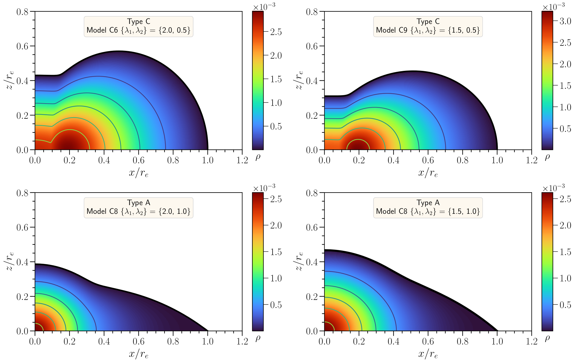
Table 1 shows the results of a convergence study for a rapidly rotating model of high compactness, constructed with the Uryu+ rotation law (14). The upper left panel of Figure 9 shows the rest mass density distribution in the $x-z$ plane, as reference, while in Figure 1 we present the angular velocity profiles $\Omega(F)$ and $\Omega(r)$ at the equatorial plane. The model has a central energy density of $\epsilon_{c}=3.3\times 10^{-3}$ and an axis ratio of $r_{p}/r_{e}=0.43$ (this is model C6 in Section 3). We demonstrate the convergence of the following quantities with increasing resolution: the central energy density $\epsilon_{c}$, the maximum energy density $\epsilon_{\text{max}}$, the gravitational mass $M$, the rest mass $M_{0}$, the angular momentum $J$ and the ratio of the rotational kinetic energy $T$ over the absolute value of the gravitational binding energy $|W|$, the angular velocity at the rotation axis $\Omega_{c}$, the maximum value of angular velocity $\Omega_{\text{max}}$, the angular velocity at the equator $\Omega_{e}$, the angular velocity of a free particle in circular orbit at the equator $\Omega_{K}$, the circumferential radius $R_{e}$, the coordinate radius $r_{e}$ at the equator and the 3-dimensional general relativistic virial index GRV3. The latter has been shown to reflect the accuracy of numerical models of stationary equilibrium configurations (Nozawa et al. 1998).

For the convergence study we use $(s,\mu)$ grids of $({\tt SDIV}\times{\tt MDIV})$=$(201\times 101)$, $(401\times 201)$, $(801\times 401)$ and $(1601\times 801)$. Our results demonstrate 2nd-order convergence, as expected for the overall numerical schemes employed in rns. Between the two highest resolutions, the relative difference is less than $\sim 2.6\times 10^{-5}$ for the integrated quantities $M,M_{0},J,T/|W|$ (in particular, for the masses it is less than $\sim 2\times 10^{-6}$) and less than $\sim 2.3\times 10^{-5}$ for the local quantities $r_{e},R_{e},\Omega_{c},\Omega_{\text{{max}}},\Omega_{e},\Omega_{K}$.

In the remainder of this work, all numerical models will be constructed with a standard resolution of $({\tt SDIV}\times{\tt MDIV})$=$(801\times 401)$.

For comparison with previous work (Stergioulas et al. 2004; Iosif & Stergioulas 2014), we construct three sequences of equilibrium models using the new differential rotation law (14):

• •

  Sequence A is a constant rest mass sequence with $M_{0}=1.506$.

• •

  Sequence B is a constant central energy density sequence with $\epsilon_{c}=1.444\times 10^{-3}$.

• •

  Sequence C is a constant central energy density sequence with $\epsilon_{c}=3.3\times 10^{-3}$.

We note that the central energy density value of sequence C, which is the most relativistic out of the three sequences, is determined taking into account remarks in Takami et al. 2011 and Giacomazzo et al. 2011 concerning the location of the secular and dynamical instabilities. We note that the faster rotating equilibrium models of sequence C could be both secularly and dynamically unstable. For the KEH rotation law, Weih et al. 2018 showed that the dynamical instability occurs well before the turning points of constant-angular-momentum sequences¹¹ 1 The latter are used to locate the secular axisymmetric instability in uniformly rotating stars.. See also Friedman & Stergioulas 2013 for a summary on axisymmetric stability and turning points, where the difference between indices $\Gamma$ (governing the equilibrium EOS) and $\Gamma_{1}$ (governing dynamical oscillations) is highlighted. This means that for realistic (i.e. hot) stars the instability limit will not be the same as in the case of cold stars. In particular, the difference between secular and dynamical instability for hot stars could be larger than the corresponding difference for cold stars.

Tables 2 and 4 list all relevant physical quantities for the three different sequences of equilibrium models. Since we want to compare these models to the corresponding models constructed with the KEH rotation law, we re-calculated sequences A, B (defined in Stergioulas et al. 2004) and C (defined in Iosif & Stergioulas 2014) with the KEH rotation law, using our standard resolution of $({\tt SDIV}\times{\tt MDIV})$=$(801\times 401)$. For the KEH sequence A, we kept the same central energy density values and a rest mass of $M_{0}=1.506$ as in Stergioulas et al. 2004, which resulted in slightly different $r_{p}/r_{e}$ (due to the different resolution) than those reported in Stergioulas et al. 2004. In addition, for the KEH sequence C, we calculated an additional model with $r_{p}/r_{e}=0.43$, in order to facilitate the comparison with the Uryu+ sequence C for the case of $\{\lambda_{1},\lambda_{2}\}=\{2.0,0.5\}$ (Figures 5 and 7), since the latter terminates at this axis ratio²² 2 The termination of sequence C with the Uryu+ rotation law is due to a limitation of the numerical scheme in rns - the sequence has not reached the mass-shedding limit, as is evident from the $\Omega_{e}$ vs. $\Omega_{K}$ values of model C6 displayed in Table 4.. The detailed properties of this additional model are displayed in Table 6 in Appendix C. In the Figures 2, 3, 4, 5, 6 and 7 that follow, all models have been constructed assuming $\{\lambda_{1},\lambda_{2}\}=\{2.0,0.5\}$.

In Figure 2 we plot the gravitational mass $M$ as a function of the central energy density $\epsilon_{c}$ for the three sequences A, B and C. For reference, we show the TOV (nonrotating) sequence as a solid line and the mass-shedding limit for uniform rotation (Kepler limit) as a dashed line. The dotted line represents the axisymmetric stability limit for uniformly rotating models, based on the turning point method by Friedman et al. 1988, see also models S1-S4 in (Baiotti et al. 2005, Table I).

Figure 3 shows a comparison of the stellar surfaces for representative models of each sequence with an $r_{p}/r_{e}$ ratio of $\sim 0.5$, between the Uryu+ differential rotation law and the KEH law. The Uryu+ models have a smaller radius and the surface near the rotation axis has a stronger quasi-toroidal shape than the corresponding KEH models. Note that, based on the density distribution in the equatorial plane, model A9 would be classified as quasi-spherical for the KEH law with $r_{p}/r_{e}=0.5133$ and marginally quasi-toroidal for the Uryu+ law with $r_{p}/r_{e}=0.4882$, whereas model B10 ($r_{p}/r_{e}=0.5$) would be quasi-spherical for KEH and quasi-toroidal for the Uryu+ law and model C5 ($r_{p}/r_{e}=0.5$) would be classified as quasi-toroidal for both rotation laws. The adoption of the Uryu+ law thus has the tendency to produce quasi-toroidal models earlier along a sequence of equilibrium models that starts at the nonrotating sequence.

Figures 4 and 5 show a comparison of the gravitational mass $M$ along the three equilibrium sequences A, B and C, for models constructed with the Uryu+ and KEH differential rotation laws. Data for the relative physical quantities for the KEH law, appear in Stergioulas et al. 2004; Iosif & Stergioulas 2014. We find that the difference in gravitational mass between the two rotation laws is very small, for all three sequences, when one interchanges the two rotation laws.

Figures 6 and 7 compare the mass-radius relations for the three sequences A, B and C, constructed with the two rotation laws. A general remark is that all models using the Uryu+ differential rotation law (14) have consistently smaller radii than their counterparts constructed with the KEH law. The relative differences are larger for the rapidly rotating, low-density models of sequence A, where they can exceed $10\%$. For sequence B, the relative differences in radii between the two differential rotation laws, range from $3\%$ to $7\%$ for models with axis ratio between $r_{p}/r_{e}\sim 0.7$ and $\sim 0.5$, respectively. For sequence C the corresponding relative differences are at the $2\%$ and $4\%$ levels, owing to the greater compactness of the sequence.

The models defined in Sec. 3.1 and explored in Sec. 3.2 were constructed with the specific choice of $p=1,q=3$ and $\lambda_{1}=2.0,\lambda_{2}=0.5$. Here, we explore the impact of varying $\lambda_{1}$ and $\lambda_{2}$, while keeping $p=1,q=3$ fixed, by first focusing on selected equilibrium models from each sequence with $r_{p}/r_{e}\sim 0.7$ and $\sim 0.5$. Table 3 summarises our results for representative models of sequences A and B with axis ratio values of 0.7 and 0.5, while full sequence C variations are explored in Table 4. We pick two values for the first parameter $\lambda_{1}=\{2.0,1.5\}$ and two values for the second parameter $\lambda_{2}=\{0.5,1.0\}$, leading to four distinct pairs of $(\lambda_{1},\lambda_{2})$. This is motivated by the differences in rotational profiles seen in numerical simulations of post-merger remnants, when different EOS and total masses are used, see the examples in Hanauske et al. 2017; De Pietri et al. 2020.

Models A5, B6 in Table 3, and C3 in Table 4 have $r_{p}/r_{e}\sim 0.7$. Between the different $\{\lambda_{1},\lambda_{2}\}$ runs, we notice variations in all the equilibrium quantities. The most striking difference is the fact that the equatorial radii are increasing with decreasing $\lambda_{1}$ and increasing $\lambda_{2}$. Increasing $\lambda_{2}=\Omega_{e}/\Omega_{c}$ leads to a larger radius increase, compared to the corresponding increase in radius when $\lambda_{1}=\Omega_{\text{max}}/\Omega_{c}$ decreases.

Models A9, B10 in Table 3 and C5 in Table 4 have $r_{p}/r_{e}\sim 0.5$. The increase of the equatorial radii with decreasing $\lambda_{1}$ and with increasing $\lambda_{2}$ is also present here, with the effect magnified due to the faster rotation. Again, increasing $\lambda_{2}=\Omega_{e}/\Omega_{c}$ leads to a larger radius increase, compared to the corresponding increase in radius when $\lambda_{1}=\Omega_{\text{max}}/\Omega_{c}$ decreases. The difference in masses (both gravitational and rest mass) between the different $\{\lambda_{1},\lambda_{2}\}$ runs, is more pronounced in the low-density configuration A9 compared to the other two models B10 and C5 that are more compact. An important observation is that while these models are quasi-toroidal for the choice $\{\lambda_{1},\lambda_{2}\}=\{2.0,0.5\}$, they are quasi-spherical for the other three $\{\lambda_{1},\lambda_{2}\}$ options we consider here (since $\epsilon_{c}=\epsilon_{\text{max}}$).

In Figure 8 we present the effect of the different $\lambda_{1}$ and $\lambda_{2}$ options on the energy density and angular velocity profiles in the equatorial plane, for the three models A9, B10 and C5 with $r_{p}/r_{e}\sim 0.5$.³³ 3 Depending on the cut-off density, the EOS and the total mass, the axis ratio $r_{p}/r_{e}$ of post-merger remnants in simulations is roughly in the range between $\sim 0.5$ and $\sim 0.7$.. The figures in the left column of Figure 8 show the energy density profile $\epsilon(r)$ for the four different $\{\lambda_{1},\lambda_{2}\}$ pairs considered. As we already pointed out, apart from the default option $\{\lambda_{1},\lambda_{2}\}=\{2.0,0.5\}$ that yields quasi-toroidal configurations for models A9, B10 and C5, the other three $\{\lambda_{1},\lambda_{2}\}$ pairs result in quasi-spherical configurations for the same $\epsilon_{c}$ and $r_{p}/r_{e}$ values. The figures in the right column of Figure 8 show the corresponding angular velocity profile $\Omega(r)$ for the four distinct $\{\lambda_{1},\lambda_{2}\}$ pairs for each of the three chosen models, demonstrating in essence the different degrees of differential rotation considered. We notice that any choice other than the default $\{\lambda_{1},\lambda_{2}\}=\{2.0,0.5\}$, results in larger radii, with respect to this choice.

In order to probe whether the morphology of the selected models A9, B10 and C5 falls into the spheroidal or quasi-toroidal category, we kept each model’s central energy density fixed and constructed additional configurations at lower axis ratios for each of the four pairs $\{\lambda_{1},\lambda_{2}\}$ under study. For the three values of central energy density considered (i.e. model A9’s $\epsilon_{c}=0.396\times 10^{-3}$, model B10’s $\epsilon_{c}=1.444\times 10^{-3}$ and model C5’s $\epsilon_{c}=3.3\times 10^{-3}$) we found that both $\{\lambda_{1},\lambda_{2}\}$ variations with $\lambda_{2}=0.5$ (i.e. the pairs $\{2.0,0.5\}$ and $\{1.5,0.5\}$) exhibited strong quasi-toroidal characteristics at axis ratios lower than 0.5. Respectively, both $\{\lambda_{1},\lambda_{2}\}$ variants with $\lambda_{2}=1.0$ (i.e. the pairs $\{2.0,1.0\}$ and $\{1.5,1.0\}$) came gradually closer to the mass-shedding limit, as the axis ratio was reduced below 0.5, while remaining quasi-spherical. This behaviour is reminiscent of different types of solutions in the Ansorg et al. 2009 classification scheme (where four different types of solutions, A, B, C and D were identified) and encourages a more thorough investigation of variants of complete sequences of models with different $\{\lambda_{1},\lambda_{2}\}$ options, which we provide in the following Section.

Having performed an initial exploration for selected equilibrium models, of the effect that different values for the parameters $\{\lambda_{1},\lambda_{2}\}$ have, we now construct variants of the complete sequence C, employing four different pairs of $\{\lambda_{1},\lambda_{2}\}$. Our results for the four variants are reported in Table 4.

For the cases of $\{\lambda_{1},\lambda_{2}\}=\{1.5,1.0\}$ and $\{2.0,1.0\}$ we find that the sequence reaches the mass-shedding limit (where $\Omega_{e}=\Omega_{K}$) at an axis ratio $r_{p}/r_{e}$ of 0.46693 and 0.38602, correspondingly. From Table 4, we notice that the these models at the mass-shedding limit are still quasi-spherical ($\epsilon_{c}=\epsilon_{\text{{max}}}$). The lower panels of Figure 9 show that the two-dimensional rest-mass density distributions of these two models at the mass-shedding limit feature the characteristic cusp in the equatorial plane. In addition, the lower panels of Figure 10 show the shape of the surface for all members of the two variants of sequence C that terminate at the mass-shedding limit. Evidently, these two variants of sequence C remain quasi-spherical, up to mass-shedding. We conclude that the variants of sequence C calculated with $\{\lambda_{1},\lambda_{2}\}=\{1.5,1.0\}$ and $\{\lambda_{1},\lambda_{2}\}=\{2.0,1.0\}$ can be classified as type A solutions⁴⁴ 4 We caution that our terminology of ”sequence A” should not be confused with the terminology of ”type A solutions”. , according to the classification of Ansorg et al. 2009.

For the variant of sequence C with $\{\lambda_{1},\lambda_{2}\}=\{2.0,0.5\}$, quasi-toroidal models appear already at $r_{p}/r_{e}=0.5$ (see Table 4, where for model C5 of this variation, $\epsilon_{c}<\epsilon_{\text{{max}}}$, i.e. the maximum density is off-center). The upper left panel of Figure 9 shows the meridional rest mass density distribution for the terminal model of this variation (model C6 with $r_{p}/r_{e}=0.43$). The corresponding panel of Figure 10 shows that the shape of the surface for the members of this sequence is transitioning from quasi-spheroidal models at high axis ratio to quasi-toroidal models at low axis ratio. Since the mass-shedding limit has not been reached (see Table 4), even though the models have become quasi-toroidal, we classify the models belonging to this variant of sequence C as type C solutions⁵⁵ 5 We caution that our terminology of ”sequence C” should not be confused with the terminology of ”type C solutions”., following Ansorg et al. 2009.

For the variant of sequence C with $\{\lambda_{1},\lambda_{2}\}=\{1.5,0.5\}$ the situation is similar to the case of $\{\lambda_{1},\lambda_{2}\}=\{2.0,0.5\}$. After constructing the initial quasi-spheroidal models of this family (i.e. models with $r_{p}/r_{e}>0.5$ where $\epsilon_{c}=\epsilon_{\text{{max}}}$, see Table 4) we performed a search starting from an axis ratio value of 0.5 and decreased $r_{p}/r_{e}$ using a 0.01 step. We noticed a local maximum in the energy density profile at the equatorial plane gradually rising and when the axis ratio reached the value 0.41, the maximum density was found to be definitively off-center. This marked the transition to quasi-toroidal configurations. We kept on decreasing the axis ratio, down to a value of 0.31, where the rns code ceased producing models for this choice of parameters. The upper right panel of Figure 9 shows the meridional rest mass density distribution for the terminal model C9 (with $r_{p}/r_{e}=0.31$). Models constructed with $0.41>r_{p}/r_{e}\geq 0.31$ exhibited a gradually “stronger” quasi-toroidal morphology (see upper right panel of Figure 10), while $\Omega_{e}$ always remained smaller than $\Omega_{K}$. We note that for the terminal model C9, we have $\Omega_{e}/\Omega_{K}\simeq 0.77$, i.e. no mass-shedding limit is encountered. Thus, we classify the variant of sequence C, calculated with $\{\lambda_{1},\lambda_{2}\}=\{1.5,0.5\}$, as a type C solution, according to Ansorg et al. 2009.

References

- Abbott et al. (2017a) Abbott B. P., et al., 2017a, Phys. Rev. Lett., 119, 161101
- Abbott et al. (2017b) Abbott B. P., et al., 2017b, ApJL, 848, L13
- Ansorg et al. (2009) Ansorg M., Gondek-Rosińska D., Villain L., 2009, MNRAS, 396, 2359
- Baiotti et al. (2005) Baiotti L., Hawke I., Montero P. J., Löffler F., Rezzolla L., Stergioulas N., Font J. A., Seidel E., 2005, Phys. Rev. D, 71, 024035
- Baumgarte et al. (2000) Baumgarte T. W., Shapiro S. L., Shibata M., 2000, ApJ, 528, L29
- Bauswein & Janka (2012) Bauswein A., Janka H. T., 2012, Phys. Rev. Lett., 108, 011101
- Bauswein & Stergioulas (2015) Bauswein A., Stergioulas N., 2015, Phys. Rev. D, 91, 124056
- Bauswein & Stergioulas (2017) Bauswein A., Stergioulas N., 2017, MNRAS, 471, 4956
- Bauswein & Stergioulas (2019) Bauswein A., Stergioulas N., 2019, J. Phys. G: Nucl. Part. Phys., 46, 113002
- Bauswein et al. (2012) Bauswein A., Janka H. T., Hebeler K., Schwenk A., 2012, Phys. Rev. D, 86, 063001
- Bauswein et al. (2016) Bauswein A., Stergioulas N., Janka H.-T., 2016, Eur. Phys. J. A, 52, 56
- Bernuzzi (2020) Bernuzzi S., 2020, Gen. Relativ. Gravit., 52, 108
- Bernuzzi et al. (2014) Bernuzzi S., Dietrich T., Tichy W., Brügmann B., 2014, Phys. Rev. D, 89, 104021
- Bozzola et al. (2018) Bozzola G., Stergioulas N., Bauswein A., 2018, MNRAS, 474, 3557
- Camelio et al. (2019) Camelio G., Dietrich T., Marques M., Rosswog S., 2019, Phys. Rev. D, 100, 123001
- Camelio et al. (2021) Camelio G., Dietrich T., Rosswog S., Haskell B., 2021, Phys. Rev. D, 103, 063014
- Ciolfi (2020) Ciolfi R., 2020, Gen. Relativ. Gravit., 52, 59
- Ciolfi et al. (2017) Ciolfi R., Kastaun W., Giacomazzo B., Endrizzi A., Siegel D. M., Perna R., 2017, Phys. Rev. D, 95, 063016
- Ciolfi et al. (2019) Ciolfi R., Kastaun W., Kalinani J. V., Giacomazzo B., 2019, Phys. Rev. D, 100, 023005
- Cook et al. (1992) Cook G. B., Shapiro S. L., Teukolsky S. A., 1992, ApJ, 398, 203
- De Pietri et al. (2016) De Pietri R., Feo A., Maione F., Löffler F., 2016, Phys. Rev. D, 93, 064047
- De Pietri et al. (2020) De Pietri R., Feo A., Font J. A., Löffler F., Pasquali M., Stergioulas N., 2020, Phys. Rev. D, 101, 064052
- Dietrich et al. (2015) Dietrich T., Bernuzzi S., Ujevic M., Brügmann B., 2015, Phys. Rev. D, 91, 124041
- East et al. (2016) East W. E., Paschalidis V., Pretorius F., Shapiro S. L., 2016, Phys. Rev. D, 93, 024011
- East et al. (2019) East W. E., Paschalidis V., Pretorius F., Tsokaros A., 2019, Phys. Rev. D, 100, 124042
- Endrizzi et al. (2016) Endrizzi A., Ciolfi R., Giacomazzo B., Kastaun W., Kawamura T., 2016, Class. Quantum Gravity, 33, 164001
- Endrizzi et al. (2018) Endrizzi A., Logoteta D., Giacomazzo B., Bombaci I., Kastaun W., Ciolfi R., 2018, Phys. Rev. D, 98, 043015
- Espino & Paschalidis (2019) Espino P. L., Paschalidis V., 2019, Phys. Rev. D, 99, 083017
- Espino et al. (2019) Espino P. L., Paschalidis V., Baumgarte T. W., Shapiro S. L., 2019, Phys. Rev. D, 100, 043014
- Friedman & Stergioulas (2013) Friedman J. L., Stergioulas N., 2013, Rotating Relativistic Stars. Cambridge Monographs on Mathematical Physics, Cambridge University Press, doi:10.1017/CBO9780511977596
- Friedman & Stergioulas (2020) Friedman J. L., Stergioulas N., 2020, Int. J. Mod. Phys. D, 29, 2041015
- Friedman et al. (1988) Friedman J. L., Ipser J. R., Sorkin R. D., 1988, ApJ, 325, 722
- Fujibayashi et al. (2018) Fujibayashi S., Kiuchi K., Nishimura N., Sekiguchi Y., Shibata M., 2018, ApJ, 860, 64
- Galeazzi et al. (2012) Galeazzi F., Yoshida S., Eriguchi Y., 2012, A&A, 541, A156
- Giacomazzo et al. (2011) Giacomazzo B., Rezzolla L., Stergioulas N., 2011, Phys. Rev. D, 84, 024022
- Goldstein et al. (2017) Goldstein A., et al., 2017, ApJL, 848, L14
- Hanauske et al. (2017) Hanauske M., Takami K., Bovard L., Rezzolla L., Font J. A., Galeazzi F., Stöcker H., 2017, Phys. Rev. D, 96, 043004
- Hotokezaka et al. (2011) Hotokezaka K., Kyutoku K., Okawa H., Shibata M., Kiuchi K., 2011, Phys. Rev. D, 83, 124008
- Hotokezaka et al. (2013) Hotokezaka K., Kiuchi K., Kyutoku K., Muranushi T., Sekiguchi Y.-i., Shibata M., Taniguchi K., 2013, Phys. Rev. D, 88, 044026
- Iosif & Stergioulas (2014) Iosif P., Stergioulas N., 2014, Gen. Relativ. Gravit., 46, 1800
- Isenberg (2008) Isenberg J. A., 2008, Int. J. Mod. Phys. D, 17, 265
- Kaplan et al. (2014) Kaplan J. D., Ott C. D., O’Connor E. P., Kiuchi K., Roberts L., Duez M., 2014, ApJ, 790, 19
- Karkowski et al. (2018) Karkowski J., Kulczycki W., Mach P., Malec E., Odrzywołek A., Piróg M., 2018, Phys. Rev. D, 97, 104017
- Kastaun & Galeazzi (2015) Kastaun W., Galeazzi F., 2015, Phys. Rev. D, 91, 064027
- Kastaun et al. (2016) Kastaun W., Ciolfi R., Giacomazzo B., 2016, Phys. Rev. D, 94, 044060
- Kastaun et al. (2017) Kastaun W., Ciolfi R., Endrizzi A., Giacomazzo B., 2017, Phys. Rev. D, 96, 043019
- Kiuchi et al. (2018) Kiuchi K., Kyutoku K., Sekiguchi Y., Shibata M., 2018, Phys. Rev. D, 97, 124039
- Komatsu et al. (1989) Komatsu H., Eriguchi Y., Hachisu I., 1989, MNRAS, 237, 355
- Kulczycki & Malec (2020) Kulczycki W., Malec E., 2020, Phys. Rev. D, 101, 084016
- Mach & Malec (2015) Mach P., Malec E., 2015, Phys. Rev. D, 91, 124053
- Nozawa et al. (1998) Nozawa T., Stergioulas N., Gourgoulhon E., Eriguchi Y., 1998, A&AS, 132, 431
- Paschalidis & Stergioulas (2017) Paschalidis V., Stergioulas N., 2017, Living Rev. Relativ., 20, 7
- Paschalidis et al. (2015) Paschalidis V., East W. E., Pretorius F., Shapiro S. L., 2015, Phys. Rev. D, 92, 121502
- Passamonti & Andersson (2020) Passamonti A., Andersson N., 2020, MNRAS, 498, 5904
- Radice (2017) Radice D., 2017, ApJL, 838, L2
- Radice (2020) Radice D., 2020, Symmetry, 12
- Radice et al. (2018) Radice D., Perego A., Bernuzzi S., Zhang B., 2018, MNRAS, 481, 3670
- Sekiguchi et al. (2011) Sekiguchi Y., Kiuchi K., Kyutoku K., Shibata M., 2011, Phys. Rev. Lett., 107, 051102
- Shibata & Hotokezaka (2019) Shibata M., Hotokezaka K., 2019, Annu. Rev. Nucl. Part. Sci., 69, 41
- Shibata & Kiuchi (2017) Shibata M., Kiuchi K., 2017, Phys. Rev. D, 95, 123003
- Shibata et al. (2017) Shibata M., Kiuchi K., Sekiguchi Y.-i., 2017, Phys. Rev. D, 95, 083005
- Stergioulas & Friedman (1995) Stergioulas N., Friedman J. L., 1995, ApJ, 444, 306
- Stergioulas et al. (2004) Stergioulas N., Apostolatos T. A., Font J. A., 2004, MNRAS, 352, 1089
- Stergioulas et al. (2011) Stergioulas N., Bauswein A., Zagkouris K., Janka H.-T., 2011, MNRAS, 418, 427
- Takami et al. (2011) Takami K., Rezzolla L., Yoshida S., 2011, MNRAS, 416, L1
- Uryū et al. (2017) Uryū K., Tsokaros A., Baiotti L., Galeazzi F., Taniguchi K., Yoshida S., 2017, Phys. Rev. D, 96, 103011
- Uryū et al. (2016) Uryū K., Tsokaros A., Galeazzi F., Hotta H., Sugimura M., Taniguchi K., Yoshida S., 2016, Phys. Rev. D, 93, 044056
- Watts et al. (2005) Watts A. L., Andersson N., Jones D. I., 2005, ApJ, 618, L37
- Weih et al. (2018) Weih L. R., Most E. R., Rezzolla L., 2018, MNRAS, 473, L126
- Wilson et al. (1996) Wilson J. R., Mathews G. J., Marronetti P., 1996, Phys. Rev. D, 54, 1317
- Xie et al. (2020) Xie X., Hawke I., Passamonti A., Andersson N., 2020, Phys. Rev. D, 102, 044040
- Zhou et al. (2019) Zhou E., Tsokaros A., Uryū K., Xu R., Shibata M., 2019, Phys. Rev. D, 100, 043015
Appendix A Rescaled equations for code implementation
As in all KEH-type codes, so in the rns code, key equations and quantities are rescaled with the coordinate equatorial radius for the computations. In this appendix we summarise the relevant rescaled expressions used in this work.
The rescalings for the angular velocity , the gravitationally redshifted angular momentum per unit rest mass , the metric potentials , , and the parameters and , are given by the following expressions