Energetic spin-polarized proton beams from two-stage coherent acceleration in laser-driven plasma
Abstract
We propose a scheme to overcome the great challenge of polarization loss in spin-polarized ion acceleration. When a petawatt laser pulse penetrates through a compound plasma target consisting of a double layer slab and prepolarized hydrogen halide gas, a strong forward moving quasistatic longitudinal electric field is constructed by the self-generated laser-driven plasma. This field with a varying drift velocity efficiently boosts the prepolarized protons via a two-stage coherent acceleration process. Its merit is not only achieving a highly energetic beam but also eliminating the undesired polarization loss of the accelerated protons. We study the proton dynamics via Hamiltonian analyses, specifically deriving the threshold of triggering the two-stage coherent acceleration. To confirm the theoretical predictions, we perform three-dimensional PIC simulations, where unprecedented proton beams with energy approximating half GeV and polarization ratio 94% are obtained.
Spin is an essential intrinsic property of ions Griffiths and Schroeter 2018; Mane et al. 2005. Energetic spin-polarized proton (SPP) beams are extensively used in fundamental physics Safronova et al. 2018; Aschenauer et al. 2019 in exploring internal structures of nucleon Ji 1997; de Florian et al. 2014, nonperturbative quantum chromodynamics Adamczyk et al. 2016; Yang et al. 2017; Alexandrou et al. 2017, parity violating spin asymmetry in polarized proton colliders Adamczyk et al. 2014, and exotic phenomena within or beyond the standard model Jaeckel et al. 2020. In nuclear physics, the SPP acts as a probe to measure the cross section of nucleus interaction Rosen 1967; Tojo et al. 2002; Allgower et al. 2002, such as electron capture involved with the giant dipole resonance Glavish et al. 1972 and photon emission from nucleon bremsstrahlung Kitching et al. 1986. Additionally, SPPs have also been pursued in industrial applications, e.g., electrochemical membrane optimization Kee et al. 2013 and highly sensitive biomedical imaging Zimmer et al. 2016. Previously, energetic SPP beams were provided by traditional accelerators Bai et al. 2006 equipped with the corkscrew-like magnets, i.e., Siberian snakes Derbenev and Kondratenko 1975, to minimize proton polarization loss. The defect of such accelerators is too large in scale and budget. Therefore, an alternative compact and economical design for producing energetic SPP beams is highly desired.
Cutting-edge facilities based on the frontier optical technology Strickland and Mourou 1985; Mourou et al. 2006 can realize pulse intensity far beyond W/cm2 Danson et al. 2019, which enables low-cost and efficient laser plasma accelerators with the gradient over 100GeV/m Tajima and Dawson 1979; Esarey et al. 2009; Macchi et al. 2013. On the other side, owing to the ultraviolet photodissociation method Rakitzis et al. 2003; Sofikitis et al. 2008; Sofikitis et al. 2017; Boulogiannis et al. 2019, nuclear spin polarized hydrogen densities extended to with lifetimes near 10 ns have been achieved experimentally Sofikitis et al. 2018. Encouraged by the above two breakthroughs, there is increasing interest in high efficiency laser-driven particle acceleration Wen et al. 2019; Wu et al. 2019a; Wu et al. 2019b and spin-polarized inertial confinement fusion Hu et al. 2020 in prepolarized plasma. However, up to now, only a few schemes have been proposed to accelerate polarized protons Hützen et al. 2019; Büscher et al. 2019; Jin et al. 2020 and there is still a lack of an insightful understanding of the coulping effect between proton dynamics and collective plasma phenomena. As a result, the generated SPP beam is in low quality, with energy 50 MeV and a polarization ratio 80% Jin et al. 2020, which inevitably limits the relevant applications requiring an energetic and highly polarized proton beam Aschenauer et al. 2019; Tojo et al. 2002; Kitching et al. 1986.
In this paper, we report an approach to generate highly energetic SPP beams whose maximum energy is close to half GeV and polarization ratio is as high as 94% by utilizing a petawatt laser. When the intense pulse propagates through a compound plasma target, a strong quasi static longitudinal electric field (QSLEF) with a varying drift velocity repeatedly accelerates the polarized protons through a two-stage coherent process. Earlier, the protons are swiftly reflected by the forward moving QSLEF to arrive at a moderate velocity, while their spin polarization is largely preserved on account of the negligible net accumulation of spin modulation induced by the oscillating laser magnetic field. Later, as the drift QSLEF moves faster than these pre-accelerated protons, the protons will be caught, trapped, and reflected again by the drift QSLEF to reach higher energy. Meanwhile, a vortex plasma magnetic field, issuing in the uncompensated transverse spin precession, merely leads to a minor polarization decrease 6% for the generated SPP beam. Because net spin precession occurs within a short duration in the second stage, the realized energetic SPP beam still maintains a high polarization ratio 94%, which would significantly facilitate the development of multiple branches of physics.

The SPP dynamics is studied with the three-dimensional (3D) particle-in-cell (PIC) code Epoch Arber et al. 2015. The simulation domain 152020 is discretized into 600400400 grid cells. The compound target (s. Fig. 1a) is a double layer slab of near-critical density carbon nanotube foams Ma et al. 2007 mixed with the prepolarized HCl gas Sofikitis et al. 2018. The electron densities of the first and second layer are and , respectively. Here is the classical critical density that determines plasma opacity in nonrelativistic regime for a laser with frequency . and are the electron mass and charge. The first (second) layer target is placed at () where 40 particles per cell are chosen. The density profile of the hydrogen halides gas is a trapezoid with a flat top at and ramp on both sides, where each cell is filled with 20 particles. The electron density of the prepolarized HCl is , which is equivalent to experimentally accessible hydrogen density Sofikitis et al. 2018. The circularly polarized laser pulse of Gaussian longitudinal envelope with intensity , wavelength m, spot size and duration fs in FWHM, is focused at the plane . Considering that such an ultraintense laser usually have a few hundred femtoseconds pre-pulse with relativistic intensities before the main pulse, we perform additional 1D PIC simulations to ensure that a pre-pulse with a duration of 400 fs and intensities up to has insignificant impact on the initial condition of plasma target. Therefore, the scheme presented here for producing energetic SPP beams is valid and robust for the ultraintense pulse with a relatively high contrast ratio.
When the ultraintense pulse stably propagates inside the plasma, the drift QSLEF is sustained by the charge separation accumulated at the front edge of laser pulse as shown in Fig. 1b, where the projection displays the distribution of longitudinal electric field averaged over two laser periods at section and . The drift QSLEF , the source of accelerated proton energies, moves along the laser propagation, as in previous results Zhang et al. 2007; Robinson et al. 2008; Robinson et al. 2009; Naumova et al. 2009; Weng et al. 2012. It is convenient to characterize the proton motion in the moving frame of the drift QSLEF in one dimensional circumstance. Here, we adopt a local constant approximation, where the whole acceleration process is divided into several separate stages and in each of them the drift QSLEF is assumed to be independent on time. Thus, the properties of QSLEF are described by drift velocity , relative coordinate , field strength (), and electric potential (), where the subscript i denotes the ordinal number of stages. At each stage, after reformulating the proton dynamic equation in space, a Hamiltonian is presented as Shen et al. 2007; Gong et al. 2020, where the speed of light, the proton mass and () the downstream (upstream) boundary of electric potential. Given the conservation of Hamiltonian between points and along the separatrix, where and , the upper and lower limit momenta of protons along the contour of at the -th stage can be derived as , where and .
In order to realize the separate multiple stage proton acceleration, the connection between stages and requires that the pre-accelerated protons by the stage- can be caught up, trapped, and reaccelerated by the later stage-. From mathematical aspect, it is equivalent to the contours of and intersecting with each other. Consequently, the condition for successfully coupling these two stages are expressed as
| (1) |
where the value of can be determined once and are given. The solution of Eq.(1) is analytically derived as where
| (2) |
Here , , and are utilized. The detailed illustration of Eq.(1) and the derivation for obtaining Eq.(2) are given in the Appendix. The rainbow lines in Fig. 1c exhibit the theoretical proton trajectories in space under a two-stage coherent acceleration, where the black (blue) contour represents the distribution of Hamiltonian () at the first (second) stage. For , given that the parameters and are calculated from the moving longitudinal electric field based on the 3D PIC simulation as shown in Fig. 2(a), one can find and . Substituting these values into Eq. (2), we arrive at , which indicates the success of connecting these two separate acceleration stages.
The representative proton trajectories within time extracted from 3D PIC simulations are shown as red lines in Fig. 1d, where the background black (blue) dashed lines denote the contour of (), the same as that in Fig. 1c. The protons (in red) are reaccelereted to a momentum at fs in the second Hamiltonian after being preaccelerated to in . For comparison, green trajectories standing for the case of a uniform target with demonstrate that the protons merely experience the first stage of reflection in . Additionally, the criterion of an initially resting proton being trapped in the Hamiltonian is calculated as , and thus the yellow trajectories representing the case of exhibit that the protons quickly sliding away in are not trapped by the faster drift QSLEF.

To further understand the two-stage process, we visualize a typical proton trajectory in time resolved coordinate (s. Fig. 2a), where the background color denotes the strength of electric field at the central axis. When the laser bores a hole on the first layer slab, the proton is reflected by the laser pulse in the first stage to have a longitudinal velocity . After the laser pulse penetrates through the first layer and irradiates on the second layer slab, a faster drift QSLEF with velocity is generated to catch up with the protons and further accelerate them. The second stage of acceleration mainly occurs at which is in accordance with the location of the second layer slab. Another pronounced signal of the discontinuous two-stage acceleration is the purple line which profiles the strength of accelerating field imposed on the proton during . The upper panel of Fig. 2b shows that the proton energies increase predominantly during and , and the maximum acceleration ratio is up to 10 MeV/fs. The momentum differential averaged over the whole typical protons is illustrated in the lower panel of Fig. 2b and the maximum accelerating gradient is over 60 TeV/m. One advantage of this mechanism is the energy enhancement induced by the second stage acceleration, which is identified by the proton energy spectra at the end of two stage ( and 83 fs) in the lower panel of Fig. 2c, where the vertical dotted lines refer to the theoretically predicted maximum energy and 478 MeV in each stage. It is worth emphasizing that the key point in this mechanism is the twice occurrence of spatial coherence between the SPPs and the drift QSLEF inside these two plasma slabs. This is far different from energetic SPP bunches driven by magnetic vortex acceleration Jin et al. 2020, where the proton energy is predominantly obtained when the laser pulse exits the rear surface of gas targets.
For the purpose of unveiling the coupling between the spin and laser-plasma effect, by utilizing Thomas-BMT equation Thomas 1927; Bargmann et al. 1959, we can characterize the proton spin dynamics as where
| (3) |
Here, is the anomalous magnetic moment for proton. The spatial distribution of spin of protons with energy MeV manifests the highly polarization of the generated energetic SPP beam (s. Fig. 2d). The upper panel of Fig. 2c presents the polarization ratio averaged over the whole protons within each energy bin. At the end of the first stage fs, the averaged spin polarization ratio is , whilst at fs the ratio . The polarization loss at fs is higher than that at fs. Detailed tracking of proton spin is illustrated below to explain the reason.
As evident from the dependence of proton spin on time in Fig. 3b, the spin deterioration are exclusively encountered at the second stage fs. Accordingly, a net increment of undesired and is pronounced at fs (s. Fig. 3c), whereas a non-ignorable oscillation takes place at the first acceleration stage fs. Considering it is instructive to examine how the governed by electric and magnetic fields, the spin differential , and is illustrated in Fig. 3d-f. In non-relativistic regime and , the cycle frequency of spin precession can be approximated as . At the first stage, and indicates that the terms incorporated with are negligible in relation and . As a result, the accumulation of undesired spin predominantly originates from the transverse magnetic field as and . The dashed black lines in Fig. 3d-f correspond to the results governed by under non-relativistic approximation, which are in reasonable agreement with the relativistic results. At the first stage, the oscillation of comes from the laser magnetic field imposed on the proton. Nevertheless, because of the periodic symmetry of the laser field, the net accumulated is inappreciable and thus the initial favorable spin characterized by is still largely preserved.

At the second stage, the oscillation symmetry in are broken (s. Fig. 3e-f) and a gradual increment occurs for (s. Fig. 3c), which is accompanied with the decrease of . The reason is that a strong vortex plasma magnetic field Pukhov and Meyer-ter Vehn 1996; Lasinski et al. 1999; Nakamura et al. 2010, sustained by the forward moving electron current when the laser pulse penetrates through the slab’s second layer, contributes to a net accumulated precession for . The distribution of magnetic field strength at fs averaged over is exhibited in Fig. 3g, where the field is along azimuthal direction and its strength is as high as 0.2 Megatesla (MT). Following the above non-relativistic assumption, we can rearrange the secondary differential of spin as and subsequently obtain the solution as
| (4) |
where and denotes the starting time of spin precession modulated by plasma vortex field . The theoretically predicted of Eq. (4) is illustrated as red dashed lines in Fig. 3a, where MT is chosen and the prediction of fs is closest to the time-resolved spin distribution obtained from PIC simulations. This further confirms that the proton polarization loss are predominantly encountered at the second acceleration stage. The distribution of undesired transverse spin of protons with energy MeV (s. Fig. 3h) demonstrates that the region with large is coincident with the strong field and is nearly neglectable near the central axis region . The red arrows in Fig. 3h mark the direction of transverse spin and its radial outward tendency is consistent with governed by the azimuthal plasma magnetic field .

To confirm the feasibility and robustness of this scheme, we examine the dependence of the acceleration efficiency on the plasma density of the first layer target. A moderate density is prioritized to achieve the high energy of the generated SPP beams (s. Fig 4a). For relatively low density , the laser pulse readily penetrates through this transparent plasma target, where protons being not trapped but swiftly surpassed by the drift QSLEF is similar as the scenario of in Fig. 1d. The threshold density can be estimated via , where and are derived in relativistically transparent plasma Liu et al. 2020. Substituting and into Eq. (2), one finds and the above density threshold can be determined as (s. Fig. 4a). For relatively large density , the laser pulse would be completed depleted and reflected by the accumulated overdense plasma edge before reaching the second layer due to its finite duration fs. To estimate the density , we resort to the hole boring velocity where Robinson et al. 2009; Schlegel et al. 2009. The criterion can be interpreted as , where the first layer thickness and the interaction time. By utilizing the distance relation , the upper limit density is estimated as . Within the range of (s. Fig. 4a), the proton energy is dramatically enhanced compared with the other density conditions. In addition, the averaged spin polarization ratio (s. Fig. 4b) manifests this mechanism is favorable to preserve the proton spin polarization. predicted by Eq. (4) indicates the insignificance of precession exerted on the protons spin by the vortex plasma magnetic field within a short time. The total charge of the generated SPP beams versus plasma density (s. Fig. 4b) exhibit the similar variation tendency as that of the proton cut-off energies.
In conclusion, we identified and characterized a two-stage acceleration mechanism for generation of highly energetic SPP beams. In this scenario, the protons are accelerated by the drift QSLEF twice to achieve the energy enhancement. Meanwhile the prepolarized protons substantially preserve their initial spin orientation, because the polarization loss caused by spin precession exclusively occurs in the second acceleration stage within a relatively short time. Our mechanism based on laser-plasma acceleration, realizing a SPP beam with energy near 0.5 GeV and polarization over 90%, is an important step towards achieving the polarized ion beam quality required for the current frontiers of fundamental and nuclear physics.
Acknowledgments—This work has been supported by Natural Science Foundation of China (Grants No. 11921006 and No. 11535001) and National Grand Instrument Project (SQ2019YFF010006). The PIC code EPOCH was in part funded by the United Kingdom EPSRC Grants No. EP/G054950/1, No. EP/G056803/1, No. EP/G055165/1, and No. EP/M022463/1. The simulations are supported by High-performance Computing Platform of Peking University.
APPENDIX
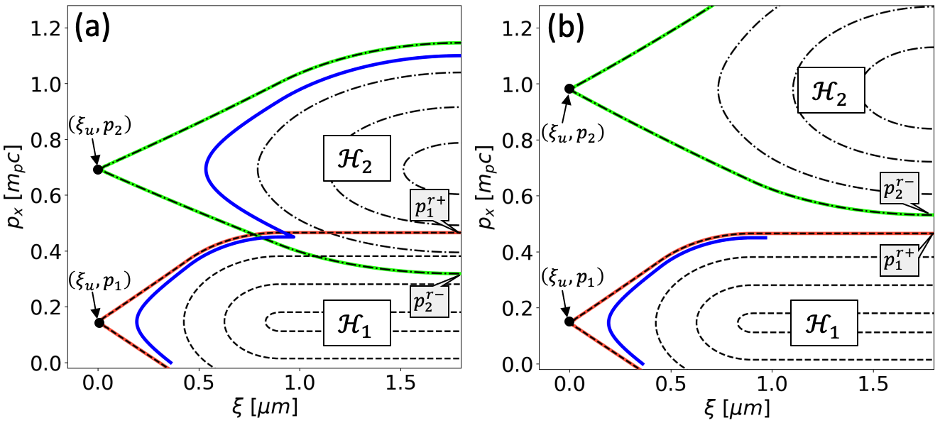
To explore the proton dynamics inside the two QSLEF in space, we adopt and to describe the Hamiltonian of proton evolving within the slow and fast QSLEF, respectively. In fact, the drift velocity of the fast QSLEF should not be so large that the protons reflected by the slow QSLEF is able to catch up and gain more energy. From the aspect of conserved Hamiltonian, to realize that the reflected protons from can be trapped and efficiently accelerated by the , the separatrix of and should intersected with each other as shown in Fig. 5(a). For simplicity, is set as in Fig. 5, where the maximum [minimum] accessible momentum on the separatrix of [] can be calculated as []. It can be found from Fig. 5(a) that the occurrence of intersection between the two separatrices is equivalent to the condition of . Therefore, the criterion for successfully coupling the proton dynamics inside these two Hamiltonian potential can be expressed as
| (5) |
where
can be found from a previous work Gong et al. 2020. Here the value of can be determined once and are given. By employing Eq.(APPENDIX), the criterion of Eq. (5) can be rearranged as
| (9) |
Then the criterion can be analytically derived as
| (10) |
where and are adopted for convenience. It worth pointing out that the threshold of Eq.(10) will return to the more general form, i.e. Eq.(2), if the subscripts and are replaced by and .
The validity of criterion Eq. 5 can also be illustrated by the numerically resolved proton trajectories in space as the solid blue lines drawn in Fig. 5. If , the proton is captured by the faster QSLEF and evolves along a contour of the as shown in Fig. 5(a). In contrast, if , the proton does not experience an efficient acceleration at the second stage characterized by as presented in Fig. 5(b). For the case exhibited in Fig. 5(a), after taking the chosen parameters , and into Eq. (10), one can find indicating that the accomplishment of repeated proton reflection inside these two Hamiltonian potential. By comparison, the parameters of the case in Fig. 5(b) is same as that in Fig. 5(a) except for , which leads to the proton reflected in on longer being reflected in . After performing this examination, we claim that the analytically derived threshold of Eq. (10) explicitly presents the condition of successfully coupling the two stage acceleration. It should be noted that at the limit of , the above threshold Eq. (10) leads to which is the upper limit velocity to achieve efficient acceleration for initially static protons Gong et al. 2020.
The realization of the two-stage coherent acceleration is determined merely by the criterion described in Eq. (2). The importance is to find the appropriate decreasing density combination of the double layer slabs, i.e. and , to provide a proper drift velocity and electric potential of the QSLEF. Some plasma kinetic effects, such as plasma instabilities Wan et al. 2020, may deteriorate this matching relation between the laser intensity and plasma density. Therefore, a detailed investigation and systematically simulations are needed to figure out the exact dependence of the acceleration efficiency and obtained proton energy on laser intensity.
References
- Griffiths and Schroeter (2018) D. J. Griffiths and D. F. Schroeter, Introduction to quantum mechanics (Cambridge University Press, 2018).
- Mane et al. (2005) S. Mane, Y. M. Shatunov, and K. Yokoya, Reports on Progress in Physics 68, 1997 (2005).
- Safronova et al. (2018) M. S. Safronova, D. Budker, D. DeMille, D. F. J. Kimball, A. Derevianko, and C. W. Clark, Rev. Mod. Phys. 90, 025008 (2018).
- Aschenauer et al. (2019) E. C. Aschenauer, S. Fazio, J. H. Lee, H. Mäntysaari, B. S. Page, B. Schenke, T. Ullrich, R. Venugopalan, and P. Zurita, Reports on Progress in Physics 82, 024301 (2019).
- Ji (1997) X. Ji, Phys. Rev. Lett. 78, 610 (1997).
- de Florian et al. (2014) D. de Florian, R. Sassot, M. Stratmann, and W. Vogelsang, Phys. Rev. Lett. 113, 012001 (2014).
- Adamczyk et al. (2016) L. Adamczyk, J. K. Adkins, G. Agakishiev, M. M. Aggarwal, Z. Ahammed, I. Alekseev, A. Aparin, D. Arkhipkin, E. C. Aschenauer, A. Attri, et al. (STAR Collaboration), Phys. Rev. Lett. 116, 132301 (2016).
- Yang et al. (2017) Y.-B. Yang, R. S. Sufian, A. Alexandru, T. Draper, M. J. Glatzmaier, K.-F. Liu, and Y. Zhao (QCD Collaboration), Phys. Rev. Lett. 118, 102001 (2017).
- Alexandrou et al. (2017) C. Alexandrou, M. Constantinou, K. Hadjiyiannakou, K. Jansen, C. Kallidonis, G. Koutsou, A. V. Avilés-Casco, and C. Wiese, Physical Review Letters 119, 142002 (2017).
- Adamczyk et al. (2014) L. Adamczyk, J. K. Adkins, G. Agakishiev, M. M. Aggarwal, Z. Ahammed, I. Alekseev, J. Alford, C. D. Anson, A. Aparin, D. Arkhipkin, et al. (STAR Collaboration), Phys. Rev. Lett. 113, 072301 (2014).
- Jaeckel et al. (2020) J. Jaeckel, M. Lamont, and C. Vallée, Nature Physics 16, 393 (2020).
- Rosen (1967) L. Rosen, Science 157, 1127 (1967).
- Tojo et al. (2002) J. Tojo, I. Alekseev, M. Bai, B. Bassalleck, G. Bunce, A. Deshpande, J. Doskow, S. Eilerts, D. E. Fields, Y. Goto, et al., Phys. Rev. Lett. 89, 052302 (2002).
- Allgower et al. (2002) C. E. Allgower, K. W. Krueger, T. E. Kasprzyk, H. M. Spinka, D. G. Underwood, A. Yokosawa, G. Bunce, H. Huang, Y. Makdisi, T. Roser, et al. (E925 Collaboration), Phys. Rev. D 65, 092008 (2002).
- Glavish et al. (1972) H. Glavish, S. Hanna, R. Avida, R. Boyd, C. Chang, and E. Diener, Physical Review Letters 28, 766 (1972).
- Kitching et al. (1986) P. Kitching, D. Hutcheon, K. Michaelian, R. Abegg, G. Coombes, W. Dawson, H. Fielding, G. Gaillard, P. Green, L. Greeniaus, et al., Physical review letters 57, 2363 (1986).
- Kee et al. (2013) R. J. Kee, H. Zhu, B. W. Hildenbrand, E. Vøllestad, M. D. Sanders, and R. P. O’Hayre, Journal of The Electrochemical Society 160, F290 (2013).
- Zimmer et al. (2016) O. Zimmer, H. M. Jouve, and H. B. Stuhrmann, IUCrJ 3, 326 (2016).
- Bai et al. (2006) M. Bai, T. Roser, L. Ahrens, I. Alekseev, J. Alessi, J. Beebe-Wang, M. Blaskiewicz, A. Bravar, J. Brennan, D. Bruno, et al., Physical review letters 96, 174801 (2006).
- Derbenev and Kondratenko (1975) Y. S. Derbenev and A. M. Kondratenko, Doklady Akademii Nauk SSSR 223, 830 (1975).
- Strickland and Mourou (1985) D. Strickland and G. Mourou, Opt. Commun. 55, 447 (1985).
- Mourou et al. (2006) G. A. Mourou, T. Tajima, and S. V. Bulanov, Rev. Mod. Phys. 78, 309 (2006).
- Danson et al. (2019) C. N. Danson, C. Haefner, J. Bromage, T. Butcher, J.-C. F. Chanteloup, E. A. Chowdhury, A. Galvanauskas, L. A. Gizzi, J. Hein, D. I. Hillier, et al., High Power Laser Science and Engineering 7 (2019).
- Tajima and Dawson (1979) T. Tajima and J. Dawson, Physical Review Letters 43, 267 (1979).
- Esarey et al. (2009) E. Esarey, C. B. Schroeder, and W. P. Leemans, Rev. Mod. Phys. 81, 1229 (2009).
- Macchi et al. (2013) A. Macchi, M. Borghesi, and M. Passoni, Reviews of Modern Physics 85, 751 (2013).
- Rakitzis et al. (2003) T. Rakitzis, P. Samartzis, R. Toomes, T. Kitsopoulos, A. Brown, G. Balint-Kurti, O. Vasyutinskii, and J. Beswick, Science 300, 1936 (2003).
- Sofikitis et al. (2008) D. Sofikitis, L. Rubio-Lago, L. Bougas, A. J. Alexander, and T. P. Rakitzis, Journal of Chemical Physics 129, 144302 (2008).
- Sofikitis et al. (2017) D. Sofikitis, P. Glodic, G. Koumarianou, H. Jiang, L. Bougas, P. C. Samartzis, A. Andreev, and T. P. Rakitzis, Phys. Rev. Lett. 118, 233401 (2017).
- Boulogiannis et al. (2019) G. K. Boulogiannis, C. S. Kannis, G. E. Katsoprinakis, D. Sofikitis, and T. P. Rakitzis, The Journal of Physical Chemistry A 123, 8130 (2019).
- Sofikitis et al. (2018) D. Sofikitis, C. S. Kannis, G. K. Boulogiannis, and T. P. Rakitzis, Phys. Rev. Lett. 121, 083001 (2018).
- Wen et al. (2019) M. Wen, M. Tamburini, and C. H. Keitel, Physical review letters 122, 214801 (2019).
- Wu et al. (2019a) Y. Wu, L. Ji, X. Geng, Q. Yu, N. Wang, B. Feng, Z. Guo, W. Wang, C. Qin, X. Yan, et al., New Journal of Physics 21, 073052 (2019a).
- Wu et al. (2019b) Y. Wu, L. Ji, X. Geng, Q. Yu, N. Wang, B. Feng, Z. Guo, W. Wang, C. Qin, X. Yan, et al., Physical Review E 100, 043202 (2019b).
- Hu et al. (2020) R. Hu, H. Zhou, Z. Tao, M. Lv, S. Zou, and Y. Ding, Phys. Rev. E 102, 043215 (2020).
- Hützen et al. (2019) A. Hützen, J. Thomas, J. Böker, R. Engels, R. Gebel, A. Lehrach, A. Pukhov, T. P. Rakitzis, D. Sofikitis, and M. Büscher, High Power Laser Science and Engineering 7 (2019).
- Büscher et al. (2019) M. Büscher, A. Hützen, I. Engin, J. Thomas, A. Pukhov, J. Böker, R. Gebel, A. Lehrach, R. Engels, T. Peter Rakitzis, et al., International Journal of Modern Physics A 34, 1942028 (2019).
- Jin et al. (2020) L. Jin, M. Wen, X. Zhang, A. Hützen, J. Thomas, M. Büscher, and B. Shen, Phys. Rev. E 102, 011201 (2020).
- Arber et al. (2015) T. Arber, K. Bennett, C. Brady, A. Lawrence-Douglas, M. Ramsay, N. Sircombe, P. Gillies, R. Evans, H. Schmitz, A. Bell, et al., Plasma Physics and Controlled Fusion 57, 113001 (2015).
- Ma et al. (2007) W. Ma, L. Song, R. Yang, T. Zhang, Y. Zhao, L. Sun, Y. Ren, D. Liu, L. Liu, J. Shen, et al., Nano Letters 7, 2307 (2007).
- Zhang et al. (2007) X. Zhang, B. Shen, X. Li, Z. Jin, and F. Wang, Physics of Plasmas 14, 073101 (2007).
- Robinson et al. (2008) A. Robinson, M. Zepf, S. Kar, R. Evans, and C. Bellei, New journal of Physics 10, 013021 (2008).
- Robinson et al. (2009) A. Robinson, P. Gibbon, M. Zepf, S. Kar, R. Evans, and C. Bellei, Plasma Physics and Controlled Fusion 51, 024004 (2009).
- Naumova et al. (2009) N. Naumova, T. Schlegel, V. Tikhonchuk, C. Labaune, I. Sokolov, and G. Mourou, Physical Review Letters 102, 025002 (2009).
- Weng et al. (2012) S. Weng, M. Murakami, P. Mulser, and Z. Sheng, New Journal of Physics 14, 063026 (2012).
- Shen et al. (2007) B. Shen, Y. Li, M. Yu, and J. Cary, Physical Review E 76, 055402 (2007).
- Gong et al. (2020) Z. Gong, Y. Shou, Y. Tang, R. Hu, J. Yu, W. Ma, C. Lin, and X. Yan, Physical Review E 102, 013207 (2020).
- Thomas (1927) L. H. Thomas, The London, Edinburgh, and Dublin Philosophical Magazine and Journal of Science 3, 1 (1927).
- Bargmann et al. (1959) V. Bargmann, L. Michel, and V. Telegdi, Physical Review Letters 2, 435 (1959).
- Pukhov and Meyer-ter Vehn (1996) A. Pukhov and J. Meyer-ter Vehn, Phys. Rev. Lett. 76, 3975 (1996).
- Lasinski et al. (1999) B. F. Lasinski, A. B. Langdon, S. P. Hatchett, M. H. Key, and M. Tabak, Physics of Plasmas 6, 2041 (1999).
- Nakamura et al. (2010) T. Nakamura, S. V. Bulanov, T. Z. Esirkepov, and M. Kando, Physical review letters 105, 135002 (2010).
- Liu et al. (2020) B. Liu, J. Meyer-ter Vehn, H. Ruhl, and M. Zepf, Plasma Physics and Controlled Fusion 62, 085014 (2020).
- Schlegel et al. (2009) T. Schlegel, N. Naumova, V. Tikhonchuk, C. Labaune, I. Sokolov, and G. Mourou, Physics of Plasmas 16, 083103 (2009).
- Wan et al. (2020) Y. Wan, I. A. Andriyash, W. Lu, W. B. Mori, and V. Malka, Phys. Rev. Lett. 125, 104801 (2020).