Hund’s coupling-assisted ferromagnetic percolation transition in a multiorbital
flat band
Abstract
By connecting Hund’s physics with flat band physics, we establish an exact result for studying ferromagnetism in a multiorbital system. We consider a two-layer model consisting of a , -orbital honeycomb lattice layer and an -orbital triangular lattice layer with sites aligned with the centers of the honeycomb plaquettes. The system features a flat band that admits a percolation representation for an appropriate chemical potential difference between the two layers. In this representation, the ground state space is spanned by maximum-spin clusters of localized single-particle states, and averaging over the ground states yields a correlated percolation problem with weights due to the spin degeneracy of the clusters. A paramagnetic-ferromagnetic transition occurs as the band approaches half filling and the ground states become dominated by states with a large maximum-spin cluster, as shown by Monte Carlo simulation.
I Introduction
Flat band physics gives rise to rich phases of matter in the presence of interactions, ranging from Mott insulating and Wigner crystal states to magnetism and fractional quantum Hall type topological states Mielke and Tasaki 1993; Mielke 1991a; Wu et al. 2007; Tang et al. 2011; Bistritzer and MacDonald 2011; Wang et al. 2013; Po et al. 2018; Tarnopolsky et al. 2019; Liu et al. 2019a; Bergman et al. 2008; Creutz 2001; Zurita et al. 2020; Chiu et al. 2020; Bergholtz and Liu 2013; Liu et al. 2014; Derzhko et al. 2015. However, reaching a rigorous theoretical understanding of many-body states in flat bands is difficult, since flat bands enhance interaction effects. As a result, nonperturbative techniques and exact results are particularly valuable.
Flat bands can often be attributed to a large number of degenerate states that are spatially localized due to destructive interference. Tight-binding models on line graphs Mielke 1991a as well as certain decorated lattices such as the Tasaki lattice Tasaki 1992 feature flat bands that can be understood through destructively interfering hopping, as can the flat bands in many more general graphs Tanaka 2020. In the presence of a repulsive on-site Hubbard interaction, these models exhibit saturated ferromagnetism when the flat band is half filled Mielke 1991b; Mielke and Tasaki 1993. Certain models such as the Tasaki lattice possess a provable ferromagnetic phase extending below half filling by realizing a direct exchange mechanism between overlapping localized states. In these models, interacting ground states are degenerate and spanned by different configurations of clusters of localized states, with the clusters independently maximizing spin Mielke 1992; Mielke and Tasaki 1993. Since the total spin of each cluster depends only on its size, the result is a correlated percolation representation that can be efficiently simulated to find the transition from paramagnetic states with small clusters at low filling to ferromagnetic states with large clusters at high filling Maksymenko et al. 2012; Liu et al. 2019b.
Orbital degrees of freedom, essential in many real materials, can be vital to the formation of a flat band, as orbital-dependent anisotropic hopping can facilitate the formation of localized states. A particular example of this is the honeycomb lattice with and orbitals at each site and orbital-dependent nearest neighbor hopping along the bond directions, where it was shown in Ref. [Wu et al. 2007] that both the lowest and highest bands are flat. The flat band degeneracy can be attributed to loop states localized around each honeycomb plaquette where the orbital at each site is oriented perpendicularly to the outgoing bond, preventing hopping out of the plaquette due to the bond-projected hopping.
However, in the presence of interactions, flat band localized states do not guarantee a provable ferromagnetic transition based on the percolation representation. Unlike in the Tasaki lattice, repulsive Hubbard interactions do not lead to an immediate percolation representation in the , -orbital honeycomb model. To take advantage of the direct exchange mechanism, Mielke and Tasaki’s scheme Mielke and Tasaki 1993 requires that no more than two flat band localized states overlap at any site and that each state satisfy a quasilocality condition, which leads to a preference for each flat band localized state to be at most singly occupied. In multiorbital systems, the conditions in Mielke and Tasaki’s scheme are often violated, which can break the percolation representation. For the -orbital honeycomb model Wu et al. 2007, the loop states violate both conditions, with three loop states overlapping at each orbital on each site. This can introduce additional states into the interacting ground state space that have lower spin within the cluster.
In this article, we show that the combination of Hund’s physics and flat band physics can allow a percolation representation to be found for multiorbital systems. We construct a two-layer model consisting of a - and -orbital honeycomb layer together with a triangular lattice -orbital layer. For appropriate chemical potential difference between the layers, the system features a flat band spanned by localized states centered on each orbital. We show that when this band is the highest energy band and at least half filled, the system admits a percolation representation in the presence of Hund’s coupling between the orbitals. This result goes beyond Mielke and Tasaki’s scheme Mielke and Tasaki 1993 and allows three localized states to overlap on site, which is useful for honeycomb lattice systems.
The remainder of this article is organized as follows. In Section II, we introduce the multiorbital flat band model with intraorbital Hubbard interactions and Hund’s coupling. We then discuss the localized single-particle flat band states that will be useful for establishing the percolation representation. In Section III, we first review Mielke and Tasaki’s scheme for percolation representations, then prove a Hund’s coupling-assisted percolation representation using the localized flat band states for our multiorbital system, and finally present Monte Carlo simulation results for the ferromagnetic percolation transition.
II Multiorbital Flat Band Model
In order to find a multiorbital flat band system that admits a percolation representation, we construct a model where the flat band is described by suitable localized states. The model system consists of spin- electrons in a two-layer system with one layer a , -orbital honeycomb lattice and the other a triangular lattice with one orbital per site. The -orbital triangular lattice sites are aligned with the centers of the -orbital honeycomb plaquettes. The set of p-orbital and f-orbital sites will respectively be labeled and , with the overall two-layer lattice .
For our model, the kinetic part of the Hamiltonian includes hopping within the - and -orbital layers as well as between nearest and orbitals, , with hopping terms depicted in Fig. 1. consists of nearest neighbor hopping between orbitals projected along the honeycomb bond direction, which describes bonding.
| (1) |
where the hopping amplitude , since the projected orbitals are odd under reflection through the bond. is the sublattice of the -orbital layer and is the projection of the , orbitals at site in the bond direction . The vectors are the nearest neighbor vectors , , . Here we take the honeycomb lattice bond length to be . This , -orbital model has been previously discussed, for example, in Refs. [Wu et al. 2007; Wu and Das Sarma 2008; Zhang et al. 2010; Zeng et al. 2021].
The orbital layer forms a triangular lattice with sites aligned with the centers of the -orbital honeycombs and features nearest-neighbor hopping given by
| (2) |
where , for reasons similar to , and are the six nearest-neighbor vectors on the -orbital triangular lattice, with and .
Hopping between layers involves nearest - and -orbital sites. Due to symmetry of the orbitals, only the orbitals directed perpendicularly to the in-plane hopping direction are involved in the hopping, as shown in Fig. 1. The hopping between the layers is then described by
| (3) |
where and with , a reordering of the vectors. In particular, when . Here are defined to be unit vectors perpendicular to with sign chosen so that is a rotation of . Thus, . The alternating sign in the hopping amplitude is due to the fact that the orbital changes sign under rotation. To interpret the model as a two-layer system, the vectors can be thought of as the -plane component of the vector between the orbitals on and the adjacent orbitals on , with the component being a small interlayer distance.

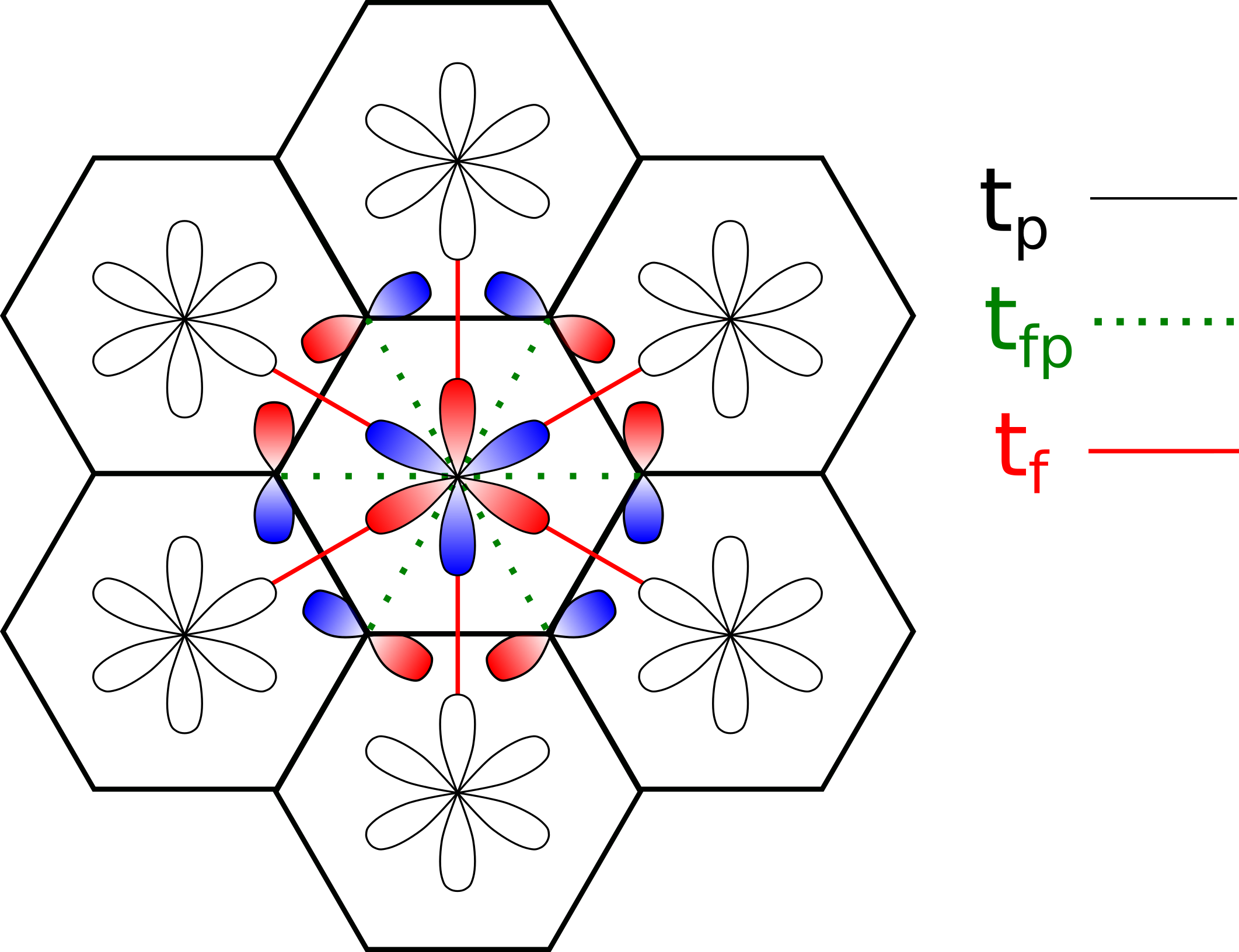
The chemical potentials for the and orbitals are given by , where the total number operator for -orbital electrons is with and a similar expression for . The total number operator for -orbital electrons is defined similarly, with . In a layered material, the chemical potential difference between the - and -orbital layers can in principle be controlled by gating. For an appropriate chemical potential difference, we will see that the model admits the desired flat band for any particular hopping amplitudes.
The on-site intraorbital Coulomb interaction is described by the Hubbard terms for and orbitals. Written in a particle-hole-symmetric form, the Hubbard interaction Hamiltonian is
| (4) | ||||
which can also be written in terms of as . This alternate expression, which separates the two-particle interaction from terms that shift the chemical potential will be convenient for studying the interacting ground states in Sec. III. We will consider only the repulsive case with .
As we will see, the intraorbital Hubbard interactions alone are not sufficient for the percolation representation we discuss in Section. III.2. The ability of the Hund’s coupling in multiorbital systems to polarize electrons in degenerate orbitals will be essential. The on-site Hund’s coupling between and orbitals is
| (5) |
where with Pauli matrices , , and the Hund’s coupling . The number operators without a spin index count both spin up and down, such as . The Hund’s coupling energy is for an on-site interorbital singlet and zero for a triplet state.
We now study the structure of the flat bands in the noninteracting model and examine the localized flat band states. In the absence of the hopping between and orbitals, the orbital layer described by is known to exhibit flat bands at energies Wu et al. 2007; Wu and Das Sarma 2008; Zhang et al. 2010. The lower flat band for spin is spanned by localized -orbital loops with alternating sign on each honeycomb, where the orbital site is used to label the surrounding honeycomb. The upper flat band is spanned by . These loop states feature a superposition of and orbitals to form a orbital perpendicular to the outgoing bond that cannot hop out due to the bond-projected hopping. These states can also be thought of as localized due to destructive interference in the , basis.
In the presence of the -orbital layer and interlayer hopping, hybridizes the - and -orbital bands. In general, this hybridization disperses the -orbital flat band at energy , while the flat band at remains flat due to destructive interference at the orbital sites. We can find conditions under which there is a flat band at an energy with eigenstates involving both and orbitals by taking the ansatz , with and determined by
| (6) | ||||
The state
| (7) |
with normalization is an eigenstate with energy as long as with
| (8) |
The state is localized to the orbital site and the neighboring orbital sites, as shown in Fig. 1. These localized states at different are degenerate and form a complete basis for the flat band with energy . To see that for all span the flat band, note that these states are linearly independent since only has nonzero amplitude at the orbital site . This set of linearly independent states has the same dimension as the flat band, the eigenspace, since one state is associated with each unit cell. This argument assumes no other bands touch the flat band, which is true for a range of parameters as we will now see by examining the dispersive bands.


When , there are five bands including the two flat bands at energies and and three dispersive bands with energies
| (9) | ||||
as shown in Fig. 2. In fact, are exactly the dispersive bands of the -orbital model Wu et al. 2007. When , the addition of the -orbital layer leaves the dispersive bands and one flat band, , of the -orbital layer unchanged, while introducing a dispersive band and involving orbitals in the remaining flat band . The flat band at energy will be useful for the percolation representation. It is the highest energy band and well separated from the lower bands when , which we will assume is the case below. In Fig. 2, the energy of the top band with a shift is plotted as a function of and , showing band curvature decreasing until the band becomes flat band at .
As we will see in the next section, the structure of the localized states in the flat band at energy allows a percolation representation to be found for the interacting ground states. At any particular orbital site , only one localized state is nonzero. This will be a valuable feature for studying the interacting system, since, using the localized states to construct many-body states, the Hubbard interaction at each orbital will give an energetic preference against doubly occupied states. The combination of Hund’s coupling and Hubbard interactions on the orbital sites will then lead to spin exchange symmetry between overlapping localized states and thus to the percolation representation.
III Ferromagnetic Percolation in Interacting Flat Bands
Before discussing the main result, we first briefly review the percolation representation in the Hubbard model studied by Mielke and Tasaki Mielke and Tasaki 1993. We then present and prove our results for the model discussed in Sec. II, where the presence of Hund’s coupling plays an important role.
III.1 Mielke-Tasaki Percolation in Flat Band Hubbard Models
For a system where the lowest-energy single-particle band is flat, a percolation representation of ferromagnetism in the flat band was found in Ref. [Mielke and Tasaki 1993] in terms of a linearly independent set of states spanning the space of the flat band. In this notation, is a lattice site and labels the state . The index set of all state labels is denoted . The percolation representation applies under two further conditions. First is quasilocality, which requires each single-particle state to have a special site in its support where every other state vanishes, i.e., for each there is an such that if and only if . Second is that no more than two states can overlap at any site, i.e., for any site there are at most two states and such that and . Two states and are said to be directly connected or overlapping if there is such a site where both states are nonzero.
Under these conditions, Ref. [Mielke and Tasaki 1993] found that if the number of electrons satisfies , the ground states of the interacting system in the presence of a repulsive single-orbital Hubbard interaction can be written as a linear superposition of states formed from clusters of single-particle states with maximum total spin.
The ground state space being spanned by the cluster states yields a percolation representation where typical ground states are paramagnetic at low filling and ferromagnetic at high filling. If filling is low, a typical ground state consists of small, independent clusters that individually maximize spin but can have low total spin. If filling is high, there is typically one macroscopic cluster dominating the total spin. In particular, if , the ground state space is spanned by fully spin-polarized states with trivial spin degeneracy. The above result from Ref. [Mielke and Tasaki 1993] thus allows for a filling-dependent ferromagnetic transition to be studied by treating the transition as a geometric percolation problem with additional spin weights due to the cluster degeneracy Maksymenko et al. 2012.
This percolation representation was proven by constructing -particle interacting states from single-particle flat band states and requiring the interacting states to have minimum Hubbard interaction energy, giving a ground state of the interacting system since the flat band minimizes the kinetic energy. In the proof of this result, the quasilocality condition is used to prevent double occupation of single-particle states, and the requirement that an overlap between single-particle states at a particular site involves only two states and yields the fact that the overall state is symmetric under swapping the spins of and , indicating maximum total spin in the cluster. Violating either of these conditions can lead to clusters with lower total spin that still have zero interaction energy.
For the model in Sec. II, the localized states shown in Fig. 1 satisfy quasilocality, as only one such state is nonzero at each orbital, but the conditions of the above theorem do not hold since three single-particle states have nonzero amplitude in the orbital component on each honeycomb lattice site . Thus, just the interaction is insufficient to produce a percolation representation of maximum-spin clusters in our multiorbital model, and we will find that the combination of and allows for a percolation representation. We note as well that the orbitals allowing quasilocality to be satisfied in the basis of localized states is necessary to find a percolation representation in terms of these localized states. Using features of the proof of our main result in Sec. III.2, we demonstrate in Appendix A an explicit example with a lower-than-maximum-spin cluster for the flat bands of the p-orbital Hamiltonian even when intraorbital Hubbard interactions and Hund’s coupling are both considered.
III.2 Hund’s Coupling-Assisted Percolation Representation
We will now see, by studying the model in Sec. II, that the presence of Hund’s coupling can allow a percolation representation to be found for certain multiorbital systems even when there are overlaps between more than two localized states on one site. The argument proceeds as follows. First, we perform a particle-hole transformation to study a model with a lowest-energy flat band. Next, we write an arbitrary ground state as a superposition of -particle states in the localized state basis. Then, we require the ground state to be a zero-energy eigenstate of the the Hund’s coupling as well as the intraorbital Hubbard interaction in the , , and orbitals. This will show that when the particle-hole-transformed flat band is at most half filled, the ground state space is spanned by states with maximum-spin clusters. Finally, we invert the particle-hole transformation to show that when the highest-energy flat band of the original system is at least half filled, the ground state space is also spanned by states with maximum-spin clusters.
Since the many-electron states used for the percolation representation will be constructed from the localized single-particle flat band states in Eq. (7), we begin by defining a creation operator for the localized state centered at site ,
| (10) | ||||
with a compact notation for -, -, and -orbital electron creation operators on the entire lattice as a -component vector. The wavefunction is compactly supported, taking nonzero values only for the orbital at and the and orbitals at for , as shown in Fig. 1. In this notation, a component of will be labeled where is a site on the lattice and is the orbital index at that site. Thus, if , and . Similarly, if , . The dot product notation is a shorthand for summing over all sites and orbitals. The subscript in identifies the localized state centered at .
The maximum-spin cluster states that will span the ground state space for appropriate filling are defined by selecting a subset and placing one single-particle localized state at each . The set can then be partitioned into , where are disjoint clusters, and two states labeled by belong to the same cluster if they are overlapping or connected by a path of overlapping states. Since total spin is maximized within each cluster, these states can be constructed from states or , depending on whether the flat band is the lowest- or highest-energy band. Here is the fully filled state and the orbital product is over , the set of all orbitals at site .
For the particle-hole transformed Hamiltonian, where the flat band is the lowest-energy band, the spin of each cluster can be lowered by a cluster spin-lowering operator with acting on , the set of orbitals where at least one state in the cluster is nonzero. For the original Hamiltonian, where the flat band is the highest-energy band, the analogous operator acting on holes is .
For the particle-hole transformed Hamiltonian, found by replacing creation and annihilation operators , , and in , we find the following theorem.
Theorem 1
Consider the particle-hole transformed Hamiltonian with and . When and , with defined in Eq. (8), the ground state space of is spanned by the states
| (11) |
with and .
One important detail is that the required in Theorem 1 is not the for which has a highest-energy flat band. Instead, there is a shift due to the additional chemical potential terms in the particle-hole-symmetric and the particle-hole-transformed Hund’s coupling . When , the single-particle terms in have a lowest-energy flat band spanned by the set of states . We have discarded additional constant terms in , as they will not affect the spectrum or chemical potential condition.
For our original model, we find the following theorem.
Theorem 2
Consider with and . When and , defined in Theorem 1, the ground state space of is spanned by
| (12) |
where , , and where are disjoint clusters.
We now proceed with the proof of Theorem 1, from which, our main result, Theorem 2 immediately follows by a particle-hole transformation. Importantly, the basis states feature maximum total spin within each cluster, since is a particle-hole transformation of and total spin commutes with particle-hole transformations, as reviewed in Appendix B.
Proof: Following Ref. [Mielke and Tasaki 1993], we construct operators canonically conjugate to by defining
| (13) | ||||
with the Gram matrix for the states . Thus, implies the canonical anticommutation relation . Note that since there is overlap between localized states centered on neighboring orbitals at and , , and will serve as a more convenient annihilation operator. The states serve as an alternate basis for the flat band, and this Gram matrix procedure is essentially a method of constructing a dual basis where each element of the dual basis is orthogonal to all but one of the vectors in the original basis. This procedure is similar to the construction of reciprocal lattice vectors from direct lattice vectors.
Now the original electron operators can be expressed in terms of the operators that annihilate the single-particle localized flat band states and operators orthogonal to the flat band. Multiplying the definition of by and summing over , can be defined to express the electron annihilation operators as
| (14) |
where with a projection out of the flat band spanned by and . Thus, . Since the ground state will be expressed in terms of operators, this construction allows the ground state condition in the presence of interactions to be analyzed using only states orthogonal or canonically conjugate to the single-particle localized flat band states.
When it is possible to construct an -electron state from single-particle flat band states that simultaneously minimizes the interactions, such a state will be a ground state, and the ground state space will be spanned by the collection of these states. In particular, the interaction and are positive semidefinite, so when there are states satisfying with energy , these states will be ground states of and can be written
| (15) |
with constraints on the coefficients to be determined by the zero-interaction-energy conditions. Here and are subsets of and or if or . If , the product over includes both, with the spin-up operator to the left. The sum over is a sum over all possible such subsets satisfying . We will see that if .
Since and are themselves sums of positive semidefinite operators at each site, we first consider the Hubbard interaction on an orbital at , which gives the condition
| (16) | ||||
since anticommutes with and with the operators in , and only when . Thus, since this condition holds for any , the state must satisfy if , or, in other words, there must be no double occupancy of localized single-particle states. If , this condition can only be met if , meaning the ground state cannot be expressed solely in terms of flat band states and must have energy higher than .
Next, we examine the Hubbard interaction in the and orbitals. Consider a honeycomb cell labeled by and examine its rightmost vertex, . Two additional honeycomb cells, centered at and , share vertex . The corresponding localized single-particle states have nonzero component in the orbital at for all three of , , and , but only and have a nonzero component at . Excluding the normalization factor on the -orbital components, the nonzero components are, and while the nonzero components are , , and . No other localized states are nonzero at .
The zero-interaction-energy condition for the -orbital Hubbard interaction at site is
| (17) | ||||
where the last line follows from the no-double-occupancy condition Eq. (16) and the fact that . The condition in Eq. (17) essentially projects out states involving a spin-singlet component between the states centered at and . Explicitly, this condition gives that for any configuration where and with , the coefficients are symmetric under exchange of spins, . Since the choice of is arbitrary, this gives the general condition that the state must have spin exchange symmetry between localized single-particle states that are nearest neighbors in the direction, states and . Eqs. (16) and (17) are equivalent to the conditions resulting from quasilocality and the requirement that no more than two single-particle states overlap at any site in Ref. [Mielke and Tasaki 1993].
The zero-interaction-energy condition for the orbitals involves three overlapping states at any site. For the orbital at site , using Eqs. (16) and (17),
| (18) | ||||
While this condition is satisfied for states that maximize spin (have spin exchange symmetry) between single-particle states at and as well as between those at and , it is not the case that every state satisfying Eq. (18) must have such spin exchange symmetry. Thus, the percolation representation is not strictly valid when the only interaction is .
The final condition we consider is . This condition can be written using only annihilation operators in by writing , where is an operator that counts whether there is a spin singlet between the and orbitals at site . The derivation of this operator identity is shown in Appendix C. In this form, is clearly a sum of positive semidefinite operators, and if and only if for every .
In terms of localized state operators, the zero-interaction-energy condition for Hund’s coupling at site is
| (19) | ||||
using the no-double-occupancy condition from Eq. (16) and the spin triplet condition between and from Eq. (17). Taking the sum and difference of the conditions in Eqs. (18) and (19) gives spin triplet conditions between and and between and . In other words, the spin degree of freedom must be fully symmetrized among any overlapping states at . This argument holds for any choice of , meaning it applies at any site in the same honeycomb sublattice as . In fact, as can be seen by considering the left-most site on the -centered honeycomb, , these spin symmetrization conditions apply both sublattices of the -orbital honeycomb lattice . If spin is symmetrized between any two overlapping localized states, a cluster of localized states will be fully spin symmetrized, since any two localized states in a cluster can be connected by a path of overlapping localized states each adjacent pair of which must have symmetrized spin. Thus, clusters of localized states have maximum total spin and ground states for can be written in the form of Eq. (11).
Theorem 2 follows immediately by particle-hole transformation. In particular, since Theorem 1 requires the lowest-energy flat band to be at most half filled, Theorem 2 requires the highest-energy flat band to be at least half filled. The clusters in Eq. (12) are then connected sets of holes, or singly-occupied localized states, surrounded by a doubly-occupied background.
In order to interpret Theorem 2 as a percolation representation, note that when the highest-energy flat band is exactly half filled, , there is a single cluster spanning the system, and all ground states have total spin . When the system is close to fully filled, clusters are small and it is easy to find combinations of basis states in Eq. (12) with low total spin. As the highest-energy flat band approaches half filling, the ground state space becomes dominated by states with a large cluster spanning the system and carrying large spin. There is thus a paramagnetic-ferromagnetic transition as the system approaches half filling of the top band from above in the sense that sufficiently close to half filling, the ground state space is dominated by states with macroscopic spin.
III.3 Monte Carlo Simulation of the Correlated Percolation Transition
With the result in Theorem 2, we can now study the ferromagnetic transition in our multiorbital model through Monte Carlo simulations for correlated percolation. The ground state basis in Theorem 2 is first reorganized into a purely geometric percolation representation by averaging over the cluster configurations and spins Mielke and Tasaki 1993; Maksymenko et al. 2012. At a fixed filling, whether typical states in the ground state space are ferromagnetic can be determined by considering the total spin averaged over the ground state space. Fixing the cluster configuration and averaging over the spins of the clusters gives that the averaged total spin of the cluster configuration, , depends only on the size of each cluster Mielke and Tasaki 1993; Maksymenko et al. 2012,
| (20) | ||||
This result can be interpreted as a geometric correlated percolation representation for the averaged ground state spin. For our model, the percolation problem is defined on the triangular lattice where a geometric configuration is specified by the set of filled sites and each configuration has a weighting factor . Since Theorem 2 applies when the highest band in the multiorbital system is at least half filled, filled sites in the percolation representation correspond to holes, or singly occupied localized states, in the multiorbital system. Similarly, empty sites in the percolation representation correspond to doubly occupied localized states in the multiorbital system. In the following discussion, we will refer directly to filled and empty sites in the percolation representation, with filling density corresponding to the hole density per unit cell of the original model.
At fixed filling , which defines the canonical ensemble, the spin averaged over all cluster configurations in the ground state space is
| (21) | ||||
with the sum over subsets with , and the weights account for cluster degeneracy. When examining the ensemble averaged spin, it will be useful to consider the spin fraction , where corresponds to a configuration with all filled sites in a single cluster.
It will also be useful to consider the grand canonical ensemble at fixed fugacity , which requires the grand canonical weights
| (22) |
and the corresponding ensemble average involving a sum over all subsets without fixing . The fugacity and the corresponding used in the grand canonical simulations couple directly to the percolation representation, or to the holes in the flat band, and are thus not related to the physical chemical potentials and .
For canonical ensemble simulations, filling is fixed, and the update step consists of an attempted swap of a randomly selected filled site with a randomly selected empty site. For grand canonical ensemble simulations at fixed , an update step consists of randomly selecting a site and attempting to fill it if empty or empty it if filled. A proposed update from configuration to is then accepted with probability or , depending on the ensemble. In both cases, simulations are done on the triangular lattice with periodic boundary conditions. Further details about the algorithm used for correlated percolation can be found in Appendix D.


Results for the canonical ensemble in a range of fillings near the transition are shown in Fig. 3(a). The spin fraction is near zero, and in fact scales to zero with system size, when , and the system is in a paramagnetic phase with typical configurations having small clusters, as shown for in Fig. 3(b). For , the spin fraction grows quickly with and typical configurations are phase separated, with a region with small clusters separated from a region with a macroscopic cluster shown for in Fig. 3(c). This phase separation behavior, which does not appear in the standard site percolation problem, has been previously observed for correlated percolation on the square lattice in Ref. Maksymenko et al. 2012, where it was understood by interpreting the weights as an effective repulsive interaction. For , the largest cluster spreads uniformly throughout the lattice, as shown for in Fig. 3(d), and the system is ferromagnetic. As , the system becomes fully spin polarized. Due to the effective repulsive interaction of the weights, the fillings and are both larger than the critical filling for standard site percolation on the triangular lattice Grimmett 1999. Since the filling in the percolation representation corresponds to hole density in the original multiorbital model, the corresponding electron densities per unit cell for the paramagnetic phase are , for phase separation are , and for the ferromagnetic phase are with fully saturated ferromagnetism at flat band half filling .

For grand canonical ensemble simulations, filling as a function of flat band fugacity is shown in Fig. 4 for triangular lattices with linear dimension . As the system size increases, the transition sharpens, suggesting a discontinuity in at a critical in the thermodynamic limit. For finite sizes, the estimate of is given by the point at which the histogram of the Monte Carlo configurations features two well defined peaks with approximately equal height, as shown in the inset of Fig. 4. For , jumps between fillings and occur at the estimated .
IV Conclusions
We have established an exact result useful for studying ferromagnetism in an interacting multiorbital flat band system. We constructed a multiorbital Hubbard model on a two-layer lattice consisting of a honeycomb lattice layer of and orbitals and a triangular lattice layer of orbitals aligned with the centers of the honeycomb plaquettes. For an appropriate chemical potential difference between the two layers, the model exhibits two flat bands due to destructive interference. The presence of Hund’s coupling between degenerate orbitals, in addition to repulsive intraorbital Hubbard interactions, allows the highest-energy flat band to admit a provable percolation representation for the degenerate many-body ground states. Ground states correspond to configurations of spin-polarized clusters of localized electron states, leading to a percolation representation for the average ground state spin. As the flat band filling varies from fully filled to half filled, the many-body ground states transition from a paramagnetic to a ferromagnetic phase, as shown by Monte Carlo simulations for correlated percolation.
Acknowledgments
We thank Tyrel McQueen for helpful discussion about potential material realizations. Simulations were performed using the Maryland Advanced Research Computing Center (MARCC) Blue Crab cluster. We acknowledge the use of the pymbar package Shirts and Chodera 2008; Chodera 2016 during data processing. This work is supported by the NSF CAREER grant DMR-1848349 and in part by the Alfred P. Sloan Research Fellowships under grant FG-2018-10971.
Appendix A Lower-spin Clusters in -orbital System
In this appendix, we consider just the - and -orbital Hamiltonian , including the -orbital kinetic Hamiltonian in Eq. (1), the intraorbital Hubbard interactions in the orbitals , as well as Hund’s coupling between orbitals in Eq. (5). By use of a simple example, we show that the loop state basis does not admit a simple percolation representation, as there are states where clusters do not maximize total spin. For consistency, we use the notation from Sec. III.2 of the main text with the modification that there are no orbital sites and is simply the set of honeycomb plaquette labels. Thus, describes the component at orbital of site of a loop state on the plaquette . All operators and are defined similarly to those in Sec. III.2 using the wavefunctions defined only at sites .
Consider an arbitrary plaquette centered at together with the six surrounding plaquettes centered at with . The nonzero components at site are and while the nonzero components are , , and , discarding the normalization factor.
The equivalents of the zero-interaction-energy conditions in Eq. (17), (18), and (19) in this case are
| (23) | ||||
These equations reduce to the conditions in the main text when there is a quasilocality site, the orbitals, that eliminates the double occupancy terms . Thus, these conditions are satisfied by states with spin exchange symmetry when there are no doubly occupied loop states, meaning states where clusters of loop states maximize spin remain ground states. There are, however, linearly independent ground states that do not maximize spin due to having a doubly occupied loop state. One such example is
| (24) |
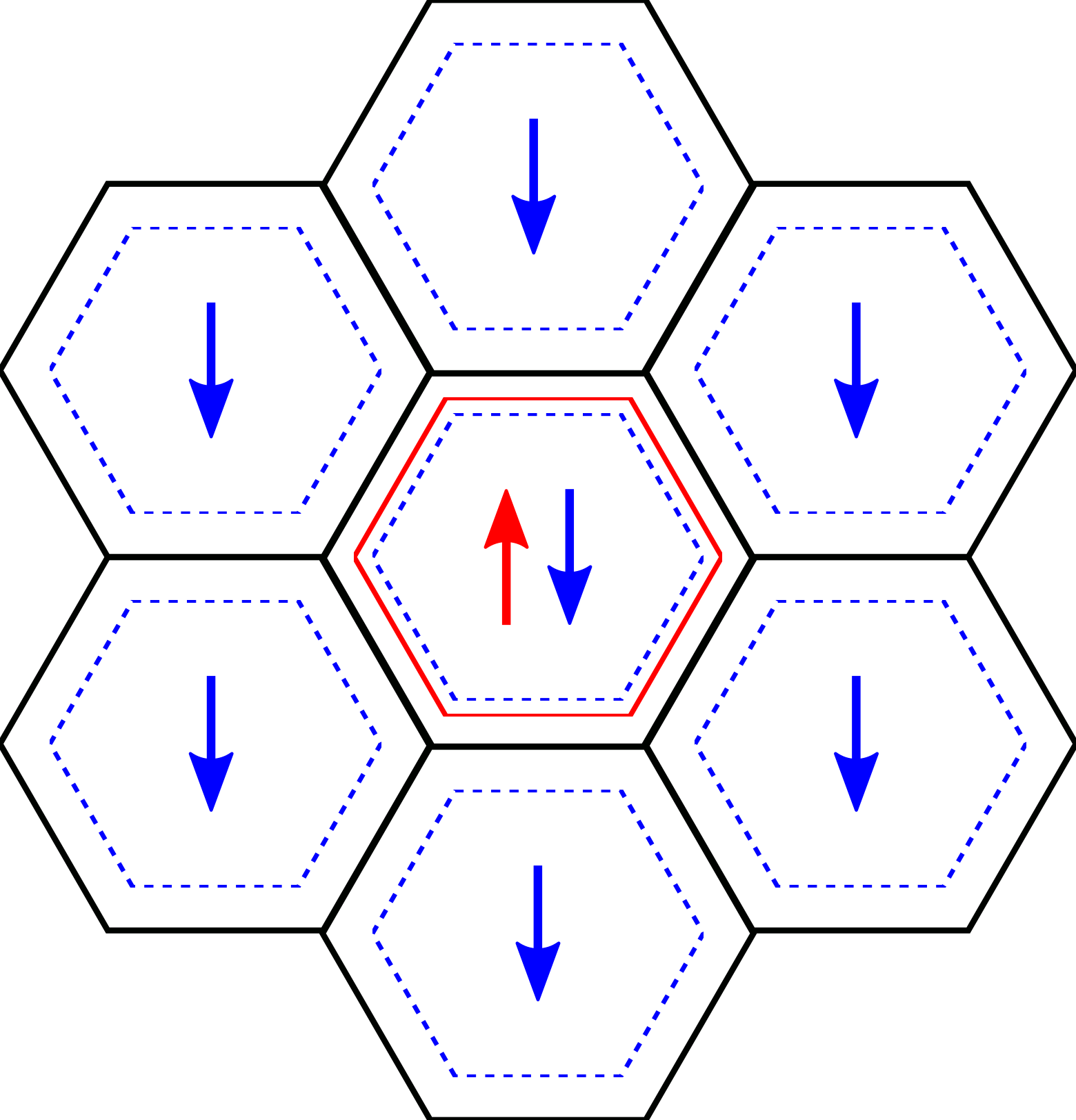
a two-particle state consisting of a spin-up loop at the plaquette surrounded by a superposition of spin-down loops at and the surrounding plaquettes, as sketched in Fig. 5. It can be verified that the state satisfies the three zero-interaction-energy conditions on every site. The conditions in Eq. (23) are satisfied by , and the conditions for the remaining sites can be shown to hold as well and follow from simple mappings. For example, the conditions at site follow from replacing , and in Eq. (23).
The two-electron state includes a component where the state is doubly occupied and has total spin . The percolation representation with maximum-spin clusters thus does not hold in the loop basis for . It should be noted that the state in Fig. 5, when written in the orbital basis rather than the loop basis, is equivalent to a two-electron state with one loop state on the central plaquette and a larger loop on the boundary of the six neighboring plaquettes. Thus, in the orbital basis, this state avoids the interaction energy trivially by avoiding doubly occupied sites. However, this state cannot be written as a superposition of maximum-spin clusters of single-plaquette loops, since it has a component where the loop is doubly occupied, and thus the percolation representation does not hold in terms of the single-plaquette loop basis.
It is important to note that the lack of a percolation representation in the loop state basis does not imply the absence of ferromagnetism in the phase diagram. Indeed, ferromagnetism at flat band half filling can be verified using Mielke’s theorem, according to which a system with a lowest- or highest-energy flat band is ferromagnetic at flat band half filling for if and only if the orthogonal projection matrix onto the flat band space is irreducible Mielke 1993; Mielke 1999; Tasaki 2020. In fact, the lack of a percolation representation in one basis in general does not prevent a percolation representation from being found in another choice of basis, though for the -orbital Hamiltonian, any other basis would likely feature overlaps between more than two states even if quasilocality were satisfied. Thus, while the -orbital system is ferromagnetic at flat band half filling, it is difficult to find a percolation representation with which the onset of ferromagnetism near flat band half filling can be studied, and the most natural basis of loop states does not admit such a representation.
Appendix B Particle-Hole Transformation of Total Spin Operator
We show here for completeness that the particle-hole transformation and total spin operators commute. For notational simplicity, consider electron operators , absorbing both the site and orbital indices into the single index . The total spin operator can be written
| (25) | ||||
which follows from the tracelessness of and the fact that . The particle-hole transformed spin operator is , which is the original spin operator with the replacement . Thus, total spin is preserved by the particle-hole transformation.
Appendix C Hund’s Coupling Operator Identity
The Hund’s coupling term is a sum of positive semidefinite operators at each honeycomb site,
| (26) | ||||
where and . takes its minimum eigenvalue of when the and orbitals at site are singly occupied and form a spin triplet state, which can be seen explicitly by using the Pauli matrix completeness identity to write
| (27) | ||||
The Hund’s coupling term can thus be written in terms of a sum of singlet number operators.
Appendix D Correlated Percolation Simulation Algorithm
In this appendix, we detail the method used for performing Monte Carlo simulations of the correlated percolation problem. The method is similar to that used in Refs. Maksymenko et al. 2012; Liu et al. 2019b. As in the main text, we are considering correlated site percolation in particular, as opposed to bond percolation. We denote the graph with the set of vertices and the set of edges. The general method does not depend on the graph structure, though the graph relevant to the main text is the triangular lattice. The correlated percolation algorithm makes use of many of the subroutines for uncorrelated percolation, particularly generating initial configurations at different fillings and labeling the clusters.
For uncorrelated percolation, sample configurations can be generated at an exact filling simply by uniformly selecting sites to fill until are filled or by filling sites and performing a random permutation Newman and Ziff 2001. These configurations are then already independent samples for uncorrelated percolation that can have clusters labeled by the Hoshen-Kopelman algorithm Hoshen and Kopelman 1976. Uncorrelated percolation in a range of filling can be efficiently simulated by generating a configuration at filling from a configuration at filling and updating the cluster labels using the Newman-Ziff algorithm Newman and Ziff 2001.
For correlated percolation, an uncorrelated percolation configuration can be used as an initial configuration and labeled using the Hoshen-Kopelman algorithm. However, as a result of the nonuniform weights, these configurations are not independent samples from the equilibrium distribution and must be moved towards equilibrium by applying an update scheme such as the Metropolis-Hastings Monte Carlo algorithm.
The graph and the configuration are stored using the following structures.
- •
Neighbor array: A 2D array of site neighbors of size , where element of the array is the site index for the th neighbor of site and is the coordination number or the maximum vertex degree in a general graph.
- •
Configuration array: An array for sites with for empty sites and a positive integer, the cluster label, for filled sites.
- •
Cluster map: A map from cluster labels to cluster values , which are nonzero integers. If , is the size of the cluster to which sites labeled belong. If , then is another cluster label belonging to the same cluster.
- •
Proper cluster label: A label with value equal to the size of the cluster containing . The proper cluster label is found from the cluster label for site by iteratively evaluating with the first label in this sequence with positive cluster value.
The cluster map scheme is central to the Hoshen-Kopelman algorithm Hoshen and Kopelman 1976. In the end, the quantities relevant to the percolation transition are the sizes of the clusters rather than the cluster labels, which can be assigned according to any convenient scheme. As clusters merge, the Hoshen-Kopelman algorithm keeps track of the new cluster sizes efficiently by using negative cluster values to avoid the need to update cluster labels for individual sites in the new cluster, and clusters are then identified by the proper cluster labels.
A simpler but less efficient scheme involves traversing all clusters. The cluster values can then all be made positive and equal to the size of the corresponding cluster, with all filled sites in a cluster sharing the same cluster label. This can be done by starting from an initial unlabeled configuration and scanning through sites on the graph, skipping empty sites as well as previously visited filled sites. When an unvisited filled site is reached, it is assigned the smallest available cluster label . The cluster containing this site is traversed by iteratively visiting filled neighbors and each site in the cluster is assigned the same cluster label . The corresponding is set to the size of this cluster.
The Hoshen-Kopelman algorithm improves efficiency by avoiding the need to fully traverse clusters to relabel filled sites when merging clusters. This is done by the following using negative cluster values to point to another label in the same cluster. When filling a site would merge multiple clusters to form a larger cluster, the total number of sites in the new cluster can be found by consulting the cluster map for the labels of each of the filled neighbors of . The smallest proper cluster label among the filled neighbors is then given the cluster value and the proper cluster labels of the remaining neighbors are all given the value . The merge thus leaves all sites in the cluster with the same proper cluster label and the need to traverse the entire cluster is avoided at the small cost of one additional cluster map lookup when finding the cluster size in the future.
Once an initial configuration at filling is generated and labeled, an equilibrium configuration of the weighted distribution in the canonical ensemble, Eq. (21), is generated by iterating the following procedure. For clarity, we refer directly to the size of the cluster containing site as , noting that is found by consulting the cluster map for label .
- 1.
Starting from configuration , select one filled site and one empty site uniformly at random.
- 2.
Empty site and calculate the weight ratio , where is the configuration with removed, as follows.
- (a)
Set the initial weight ratio value with the cluster initially containing site . Set a counter for the number of filled sites traversed.
- (b)
While the number of unvisited filled neighbors of is , pick an unvisited filled neighbor of site and perform a breadth first search (BFS) of the cluster containing .
- i.
During the search, mark visited cluster sites and count the size of the cluster .
- ii.
If during the search all neighbors of have been visited, break the loop.
- iii.
If the search completes without visiting all neighbors of , update the weight ratio and the counter .
- i.
- (c)
The size of the remaining cluster must be , and the weight is updated accordingly, .
- (a)
- 3.
Fill site and calculate the weight ratio , where is the configuration with filled, by consulting the cluster map for as follows.
- (a)
Find the proper cluster labels for each filled neighbor of and create a list of filled neighbors with one for each distinct proper cluster label. Note that is the number of clusters neighboring in .
- (b)
Store the minimum proper cluster label among proper cluster labels for the . Set . For all , set .
- (c)
Set the weight ratio .
- (a)
- 4.
Accept the trial configuration if . Otherwise accept with probability .
Explicitly filling site and updating the cluster labels can be delayed until after the updated configuration is accepted, since the relative weight for filling a site can be calculated from the cluster map before filling the site. When emptying a site , is it unfortunately necessary in the worst case to traverse all but one of the clusters neighboring , since connectivity cannot be determined by examining only the neighbors of . Since each cluster must be traversed anyway when emptying site , it is reasonable to assign a new cluster label to each traversed site of the cluster to minimize the number of negative cluster values in the cluster map. We allow early termination in the update step when all neighbors of have been visited, make use of the fact that knowing the size of the original cluster with filled means one of the clusters with empty need not be explicitly traversed. Performing a breadth first search of the clusters maximizes the chances of early termination occurring before the last cluster is traversed. As opposed to filling a site, emptying a site is performed explicitly to generate a trial configuration, since all but one of the neighboring clusters must be traversed to update the cluster labels. If the configuration is rejected, the site can simply be filled in.
Equilibrium configurations in the grand canonical ensemble at fixed fugacity , with weights given by Eq. (22), follow from an initial configuration by selecting a site uniformly at random and attempting to empty it if filled or fill it if empty, using the corresponding subroutine from the canonical ensemble simulations. The initial configuration can be randomly generated at any filling or even taken to be empty.
References
- Mielke and Tasaki (1993) A. Mielke and H. Tasaki, Commun. Math. Phys. 158, 341 (1993).
- Mielke (1991a) A. Mielke, J. Phys. A: Math. Gen. 24, L73 (1991a).
- Wu et al. (2007) C. Wu, D. Bergman, L. Balents, and S. Das Sarma, Phys. Rev. Lett. 99, 070401 (2007).
- Tang et al. (2011) E. Tang, J.-W. Mei, and X.-G. Wen, Phys. Rev. Lett. 106, 236802 (2011).
- Bistritzer and MacDonald (2011) R. Bistritzer and A. H. MacDonald, PNAS 108, 12233 (2011).
- Wang et al. (2013) Z. F. Wang, N. Su, and F. Liu, Nano Letters 13, 2842 (2013), pMID: 23678979.
- Po et al. (2018) H. C. Po, L. Zou, A. Vishwanath, and T. Senthil, Phys. Rev. X 8, 031089 (2018).
- Tarnopolsky et al. (2019) G. Tarnopolsky, A. J. Kruchkov, and A. Vishwanath, Phys. Rev. Lett. 122, 106405 (2019).
- Liu et al. (2019a) S. Liu, A. Vishwanath, and E. Khalaf, Phys. Rev. X 9, 031003 (2019a).
- Bergman et al. (2008) D. L. Bergman, C. Wu, and L. Balents, Phys. Rev. B 78, 125104 (2008).
- Creutz (2001) M. Creutz, Rev. Mod. Phys. 73, 119 (2001).
- Zurita et al. (2020) J. Zurita, C. E. Creffield, and G. Platero, Advanced Quantum Technologies 3, 1900105 (2020).
- Chiu et al. (2020) C. S. Chiu, D.-S. Ma, Z.-D. Song, B. A. Bernevig, and A. A. Houck, Phys. Rev. Research 2, 043414 (2020).
- Bergholtz and Liu (2013) E. J. Bergholtz and Z. Liu, Int. J. Mod. Phys. B 27, 1330017 (2013).
- Liu et al. (2014) Z. Liu, F. Liu, and Y.-S. Wu, Chinese Phys. B 23, 077308 (2014).
- Derzhko et al. (2015) O. Derzhko, J. Richter, and M. Maksymenko, Int. J. Mod. Phys. B 29, 1530007 (2015).
- Tasaki (1992) H. Tasaki, Phys. Rev. Lett. 69, 1608 (1992).
- Tanaka (2020) A. Tanaka, J. Stat. Phys. 181, 897 (2020).
- Mielke (1991b) A. Mielke, J. Phys. A: Math. Gen. 24, 3311 (1991b).
- Mielke (1992) A. Mielke, J. Phys. A: Math. Gen. 25, 4335 (1992).
- Maksymenko et al. (2012) M. Maksymenko, A. Honecker, R. Moessner, J. Richter, and O. Derzhko, Phys. Rev. Lett. 109, 096404 (2012).
- Liu et al. (2019b) R. Liu, W. Nie, and W. Zhang, Science Bulletin 64, 1490 (2019b).
- Wu and Das Sarma (2008) C. Wu and S. Das Sarma, Phys. Rev. B 77, 235107 (2008).
- Zhang et al. (2010) S. Zhang, H.-h. Hung, and C. Wu, Phys. Rev. A 82, 053618 (2010).
- Zeng et al. (2021) J. Zeng, M. Lu, H. Liu, H. Jiang, and X. Xie, Science Bulletin 66, 765 (2021).
- Grimmett (1999) G. Grimmett, Critical probabilities, in Percolation (Springer Berlin Heidelberg, Berlin, Heidelberg, 1999) pp. 53–76.
- Shirts and Chodera (2008) M. R. Shirts and J. D. Chodera, J. Chem. Phys. 129, 124105 (2008).
- Chodera (2016) J. D. Chodera, J. Chem. Theory Comput. 12, 1799 (2016).
- Mielke (1993) A. Mielke, Phys. Lett. A 174, 443 (1993).
- Mielke (1999) A. Mielke, J. Phys. A: Math. Gen. 32, 8411 (1999).
- Tasaki (2020) H. Tasaki, The origin of ferromagnetism, in Physics and Mathematics of Quantum Many-Body Systems (Springer International Publishing, Cham, 2020) pp. 371–455.
- Newman and Ziff (2001) M. E. J. Newman and R. M. Ziff, Phys. Rev. E 64, 016706 (2001).
- Hoshen and Kopelman (1976) J. Hoshen and R. Kopelman, Phys. Rev. B 14, 3438 (1976).