Optimal Quantum Thermometry with Coarse-grained Measurements

We take a $d$-outcome POVM $\mathcal{M}=\{M_{\alpha}\}_{\alpha=1}^{d}$ and a system in the thermal state $\tau$ of Eq. (1). Each outcome $\alpha$ then occurs with probability

$\displaystyle p_{\alpha}=\Tr(M_{\alpha}\tau).$

(4)

This distribution contains information about the temperature $T$, as quantified by the Fisher information Kullback 1968

$\displaystyle\mathcal{C}=\sum_{\alpha=1}^{d}\frac{1}{p_{\alpha}}\bigg(\frac{\partial p_{\alpha}}{\partial T}\bigg)^{2},$

(5)

which, for a thermal state, becomes Potts et al. 2019

$\displaystyle\mathcal{C}=\beta^{4}\sum_{\alpha}\frac{1}{p_{\alpha}}\big[\Tr\big(\tau M_{\alpha}(H-\langle H\rangle_{\tau})\big)\big]^{2}.$

(6)

Note that, after coarse graining, $p_{\alpha}$ is no longer in the so-called exponential family with respect to $T$¹¹ 1 In that $p_{\alpha}$ cannot be written as $\exp[\mathfrak{K}(\alpha)f(T)+\mathfrak{L}(T)+\mathfrak{M}(\alpha)]$, where $f$, $\mathfrak{K}$, $\mathfrak{L}$, and $\mathfrak{M}$ are some functions., which means that no temperature estimator can satisfy the Cramér-Rao bound for any finite number of repetitions $n$ van der Vaart 2000. However, the Fisher information ($\mathcal{C}$) is still a key precision quantifier as, for all unbiased and certain generic biased estimators, such as the maximum likelihood estimator, the Cramér-Rao bound is saturated asymptotically in the $n\to\infty$ limit. Moreover, in the same limit, the Fisher information retains its key role even in the Bayesian estimation approach²² 2 Indeed, it follows from the Bayesian Cramér-Rao bound (a.k.a. van Trees inequality) Gill and Levit 1995 that, for any estimator, in the $n\to\infty$ limit, $\Delta T\gtrsim 1/\big[n\int dT\,p(T)\mathcal{C}(T)\big]$, where $p(T)$ is the prior distribution of $T$..

We thus set as our goal to determine the optimal $d$-outcome POVM which maximises the Fisher information $\mathcal{C}$.

We first observe that the POVM elements $M_{\alpha}$ can be taken to be diagonal in the energy eigenbasis. Because $\tau$ is diagonal in this basis, only diagonal elements of $M_{\alpha}$ contribute to the probability $p_{\alpha}$ in Eq. (4). Dropping all off-diagonal elements from each $M_{\alpha}$ results in a valid POVM since the operators remain positive and still sum to identity. Hence, for every POVM, there exists a diagonal POVM which achieves the same $p_{\alpha}$ and thus the same Fisher information. It is therefore sufficient to consider diagonal POVMs when looking for an optimal POVM maximising $\mathcal{C}$.

Next, let us note that $\mathcal{C}$ is convex with respect to the POVM. That is, denoting by $\mathcal{C}_{\mathcal{M}}$ the Fisher information corresponding to a particular POVM and considering two POVMs $\mathcal{M}$ and $\mathcal{N}$ and a mixing parameter $0\leq\lambda\leq 1$, we have

$\displaystyle\mathcal{C}_{\lambda\mathcal{M}+\overline{\lambda}\mathcal{N}}\leq\lambda\mathcal{C}_{\mathcal{M}}+\overline{\lambda}\mathcal{C}_{\mathcal{N}},$

(7)

where $\overline{\lambda}=1-\lambda$. This can be seen by rewriting Eq. (6) as

$\displaystyle\mathcal{C}=\beta^{4}\sum_{\alpha}\frac{1}{p_{\alpha}}\big(W_{\alpha}\big)^{2},$

(8)

where $W_{\alpha}=\Tr\big(\tau M_{\alpha}[H-\langle H\rangle_{\tau}]\big)$. Both $p_{\alpha}$ and $W_{\alpha}$ are linear in the POVM operators. Hence, when mixing POVMs, $W_{\alpha}^{(\lambda\mathcal{M}+\overline{\lambda}\mathcal{N})}=\lambda W_{\alpha}^{(\mathcal{M})}+\overline{\lambda}W_{\alpha}^{(\mathcal{N})}$ and $p_{\alpha}^{(\lambda\mathcal{M}+\overline{\lambda}\mathcal{N})}=\lambda p_{\alpha}^{(\mathcal{M})}+\overline{\lambda}p_{\alpha}^{(\mathcal{N})}$. Equation (7) is then an immediate consequence of the fact that $\frac{1}{p}W^{2}$ is a jointly convex function of $p$ and $W$ (see, e.g., Ref. Effros 2009).

Finally, we show that the optimal POVM is necessarily a collection of nonoverlapping projectors onto eigensubspaces of $H$. Indeed, take a POVM $\mathcal{M}$ such that, for some eigenstate $|k\rangle$ of $H$, there are at least two POVM elements for which $\langle k|M_{\alpha}|k\rangle>0$. Define

$\displaystyle\varsigma_{\alpha}=\langle k|M_{\alpha}|k\rangle.$

(9)

Now, construct $d$ new POVMs $\mathcal{N}^{(\gamma)}$, with elements

$\displaystyle N^{(\gamma)}_{\alpha}=M_{\alpha}+(\delta_{\alpha\gamma}-\varsigma_{\alpha})|k\rangle\langle k|.$

(10)

Each $\mathcal{N}^{(\gamma)}$ has the property that only $N^{(\gamma)}_{\gamma}$ has a nonzero $k$’th diagonal, namely $\langle k|N^{(\gamma)}_{\gamma}|k\rangle=1$ while $\langle k|N^{(\gamma)}_{\alpha\neq\gamma}|k\rangle=0$. Furthermore, we note that

$\displaystyle\sum_{\gamma}\varsigma_{\gamma}\mathcal{N}^{(\gamma)}=\mathcal{M}.$

(11)

Since the $M_{\alpha}$ form a POVM, we have $\varsigma_{\alpha}\geq 0$ and $\sum_{\alpha}\varsigma_{\alpha}=1$. By convexity (7) of the Fisher information,

$\displaystyle\mathcal{C}_{\mathcal{M}}\leq\sum_{\gamma}\varsigma_{\gamma}\mathcal{C}_{\mathcal{N}^{(\gamma)}},$

(12)

and it follows that there must be at least one $\gamma$ for which $\mathcal{C}_{\mathcal{N}^{(\gamma)}}(T)\geq\mathcal{C}_{\mathcal{M}}(T)$. This means that the optimal POVM will have to be one that consists of nonoverlapping projectors on eigensubspaces of $H$. Given a (possibly degenerate) Hamiltonian $H=\sum_{i}E_{i}|i\rangle\langle i|$ the optimal POVM will thus be of the form

$$\Pi_{\alpha}=\sum_{E_{i}\in I_{\alpha}}|i\rangle\langle i|,$$

(13)

where the $I_{\alpha}$ define a partition of the set of all eigenenergies into nonoverlapping subsets (“bins”).

To summarize, optimal, coarse-grained thermometry can always be achieved by considering projective measurements onto nonoverlapping eigenenergy subspaces.

We now construct a method for determining the optimal eigenenergy subsets, defining the optimal POVM.

For convenience, we choose the basis of $H$ such that

$\displaystyle E_{1}\leq E_{2}\leq\cdots\leq E_{D},$

(14)

and write the probability of finding the system in bin $I_{\alpha}$ as [cf. Eq. (4)]

$\displaystyle p_{\alpha}=\Tr(\Pi_{\alpha}\tau)=\sum_{E_{i}\in I_{\alpha}}q_{i},$

(15)

where $q_{i}=\exp(-\beta E_{i})/Z$. Next, we introduce the “bin energies” (normalized average energy within each bin),

$\displaystyle\epsilon_{\alpha}=\frac{1}{p_{\alpha}}\sum_{E_{i}\in I_{\alpha}}q_{i}E_{i},$

(16)

and, with these definitions, reexpress the Fisher information in Eq. (6) for the corresponding measurement as

$\displaystyle\mathcal{C}=\beta^{4}\sum_{\alpha=1}^{d}p_{\alpha}(\epsilon_{\alpha}-\langle H\rangle)^{2}.$

(17)

We shall henceforth refer to this as the coarse-grained Fisher information. Compared with Eq. (3), the expression for $\mathcal{C}$ describes how each of the energies $\epsilon_{\alpha}$ fluctuates away from the average.

As a first step towards finding the optimal sets $I_{\alpha}$, in Appendix A, applying a result from Ref. Chakravarty et al. 1985, we prove that the best choice of $I_{\alpha}$ is given by a binning into consecutive intervals: $I_{\alpha}=\{E_{i_{\alpha-1}},E_{i_{\alpha-1}+1},\ldots,E_{i_{\alpha-1}+|I_{\alpha}|-1}\}$, where $1\leq i_{\alpha-1}\leq D$ and the iteration rule is $i_{\alpha}=i_{\alpha-1}+|I_{\alpha}|$. Introducing the “boundaries” $b_{\alpha}:=E_{i_{\alpha}}$, we can conveniently write $I_{\alpha}=[b_{\alpha-1},b_{\alpha})$, with the proviso that $b_{0}=E_{1}$ and $b_{d}=E_{D+1}=E_{D}$ (the extra level $E_{D+1}$ will not enter into any physical quantity and is introduced just so that $E_{D}$ enters $I_{d}$ despite $[b_{d-1},b_{d})$ having an open end). Note that, for discrete spectra, the boundaries $b_{\alpha}$ need not be exactly at energy eigenvalues. Positioning a boundary anywhere between neighboring eigenvalues results in the same POVM in Eq. (13).

The remaining task is then to find the optimal intervals $I_{\alpha}=[b_{\alpha-1},b_{\alpha})$ which maximize $\mathcal{C}$. This will give the best strategy for temperature estimation using a $d$-outcome POVM.

Before carrying out this optimization, it is useful to recast the problem in terms of the density of states (DOS)

$$\Omega(E)=\sum\limits_{i}\delta(E-E_{i}),$$

(18)

where $\delta$ denotes the Dirac’s delta function (note that this definition does not assume a continuous spectrum). Expectation values of any function $g(H)$ of the Hamiltonian may then be written as

$$\langle g(H)\rangle=\sum\limits_{i}g(E_{i})q_{i}=\int dEg(E)\Omega(E)\frac{e^{-\beta E}}{Z}.$$

(19)

This means that we can define the distribution of energy as

$\displaystyle q(E)=\Omega(E)\frac{e^{-\beta E}}{Z},$

(20)

so that expectation values can be computed simply in terms of integrals over $q(E)$. This way, the probabilities $p_{\alpha}$ in Eq. (15) and the bin energies in Eq. (16) can be conveniently written as

	$\displaystyle p_{\alpha}=\int_{b_{\alpha-1}}^{b_{\alpha}}\!dE\,q(E)\quad\mathrm{and}\quad\epsilon_{\alpha}=\frac{1}{p_{\alpha}}\int_{b_{\alpha-1}}^{b_{\alpha}}\!dE\,q(E)E.~$
			(21)

These quantities are therefore all expressed explicitly as functions of the boundaries $b_{\alpha}$.

The advantage of introducing the DOS is twofold. First, it allows for a unified treatment of Hamiltonians with discrete and quasi-continuous spectra (as one would expect in quantum many-body systems). Second, it allows us to frame the problem in the language of signal processing. A common task in signal processing is to transmit a continuous function $q(E)$ through a channel. Often, in order to do so, the function must be discretized into a finite set of bins $I_{\alpha}=[b_{\alpha-1},b_{\alpha})$. The question is then which choice of bins leads to the optimal transmission. This problem is solved by using the scheme known as Lloyd-Max quantization (see Ref. Gallager 2008, Chapter 3). If one uses the mean squared variations of energy as a figure of merit, one sees that the maximization of the Fisher information [see Eq. (17)] becomes entirely analogous to this signal processing problem.

To proceed, we introduce the quantity

$$\mathcal{D}=\beta^{4}\sum_{\alpha=1}^{d}\;\;\int\limits_{b_{\alpha-1}}^{b_{\alpha}}dEq(E)(E-\epsilon_{\alpha})^{2}.$$

(22)

It can be directly verified that the thermal Fisher information given by Eq. (3) can be decomposed as

$$\mathcal{F}=\mathcal{C}+\mathcal{D},$$

(23)

which means that the task of maximizing $\mathcal{C}$, for a fixed $\mathcal{F}$, is tantamount to that of minimizing $\mathcal{D}$.

The minimization can be carried out in the usual way, by equating to zero the derivatives of $\mathcal{D}$ with respect to $b_{\alpha}$. A straightforward calculation shows that the minima of $\mathcal{D}$ occur when the intervals $b_{\alpha}$ satisfy the implicit (and generally nonlinear) equations,³³ 3 The solutions to this equation are also guaranteed to be an actual minimum of $\mathcal{D}$, never a maximum. First, $\partial^{2}\mathcal{D}/\partial b_{\alpha}b_{\alpha^{\prime}}=0$ for $\alpha^{\prime}\neq\alpha$. Second, at $b_{\alpha}=(\epsilon_{\alpha+1}+\epsilon_{\alpha})/2$, we have $\partial^{2}\mathcal{D}/\partial b_{\alpha}^{2}=2\beta^{4}(\epsilon_{\alpha+1}-\epsilon_{\alpha})q(b_{\alpha})\geqslant 0$, since $q(b_{\alpha})\geqslant 0$ by construction and $\epsilon_{\alpha+1}\geqslant\epsilon_{\alpha}$ by hypothesis.

$$b_{\alpha}=\frac{\epsilon_{\alpha+1}+\epsilon_{\alpha}}{2},\qquad\alpha=1,\ldots,d-1.$$

(24)

These equations are implicit because $\epsilon_{\alpha}$ itself is a function of the $\{b_{\alpha}\}$ [Eq. (16)]. This summarizes the core of our framework. Equation (24) provides a recipe for how to optimize the energy bins in a $d$-outcome POVM in order to maximize the thermometric precision.

Let us now present two examples using our framework for optimal coarse-grained thermometry.

The two examples in Sec. III.3 carry an important general message: even measurements so coarse-grained as to have only two outcomes can estimate the temperature of a generic system with precision (as quantified by the Fisher information) that is proportional to the ultimate precision—the thermal Fisher information [Eq. (3)]. In Appendix C, we show that this is not a coincidence, by proving that any system for which the energy distribution is unimodal and has sufficiently fast decaying tails, displays a proportionality $\mathcal{C}\propto\mathcal{F}$. More specifically, we prove that there exists a finite number $\Xi\in[0,1]$ such that $\mathcal{C}\geq\Xi\mathcal{F}$.

As will be discussed in Sec. IV, the relevance of these results lies in the fact that unimodal energy distributions with quickly decaying tails are a generic behaviour expected in finite-temperature many-body systems with short-range interactions, both at and away from criticality. In fact, we will show that $\Xi=2/\pi$, as in Eq. (27), actually happens for a large variety of interacting lattice models. It is of course possible to conceive nonunimodal energy distributions for which the proportionality $\mathcal{C}\propto\mathcal{F}$ breaks down. We illustrate this in Appendix D, where we construct an example for which $\mathcal{C}/\mathcal{F}\to 0$ when $N\to\infty$.

Our framework can also be adapted to scenarios where the ideal energy binning cannot be implemented and imprecisions are present. In the simplest case, one could have some imprecision in determining the optimal bins through Eq. (24), which would lead to a decrease in $\mathcal{C}$. For the case $d=2$, this is illustrated in the inset of Fig. 3(a), which shows how $\mathcal{C}/\mathcal{F}$ decreases as the bin position deviates from its optimal value.

Another way in which imprecisions can enter our framework is when the POVMs (4) are noisy. For instance, experimental errors may cause energies close to a bin edge to sometimes result in outcomes corresponding to neighbouring bins. Such effects can be accounted for within our framework by modifying Eq. (21). To see that, we first rewrite Eq. (21) as

$\displaystyle p_{\alpha}=\int_{-\infty}^{\infty}\!dE\,q(E)B_{\alpha}(E),$

(29)

and similarly for $\epsilon_{\alpha}$. Here $B_{\alpha}(E)$ is a boxcar function, with value 1 when $E\in I_{\alpha}=[b_{\alpha-1},b_{\alpha})$, and 0 otherwise. A similar analysis can also be done at the discrete representation of Eq. (15). In this case, we would have $p_{\alpha}=\sum_{i}B_{\alpha,i}q_{i}$, where $B_{\alpha,i}$ is a matrix with entries 1 when $E_{i}\in I_{\alpha}$ and zero otherwise. However, it is more convenient to work with the continuous-energy representation (29).

It is now straightforward to generalize Eq. (29) to include the effects of noise by replacing $B_{\alpha}(E)$ by a different function. For instance, a smoothed boxcar as depicted in Fig. 4(a). Since $\sum_{\alpha}p_{\alpha}=1$ for any initial distribution $q(E)$, it follows that $\sum_{\alpha}B_{\alpha}(E)=1$ for all $E$. This can be viewed as a normalization condition for $B_{\alpha}(E)$. In fact, $B_{\alpha}(E)$ is actually a combination of a stochastic matrix (whose columns add up to one), plus an isometry, which reduces the dimension from a continuous energy $E$, to a discrete set of outcomes $\alpha$. The precise form of $B_{\alpha}(E)$ will depend on the details of the experiment.

Measurement errors can cause not only a loss of precision, but also systematic shifts in energy by, e.g., falsely displacing the energies $\epsilon_{\alpha}$ by a certain amount. For simplicity, we shall study these kinds of imprecision separately. We defer the discussion of robustness to energy shifts to Sections IV.1 and IV.2, while here we choose $B_{\alpha}(E)$ to be symmetric in the interval $[b_{\alpha-1},b_{\alpha})$, and centered at the midpoint $(b_{\alpha-1}+b_{\alpha})/2$, so that the $\epsilon_{\alpha}$’s are not displaced.

The remaining feature to describe is errors associated with imperfect binning. This can again be done using the smoothed boxcar of Fig. 4(a)

$$B_{\alpha}(E)=\frac{1}{2}\erf\left(\frac{b_{\alpha}-E}{\sigma\sqrt{2}}\right)-\frac{1}{2}\erf\left(\frac{b_{\alpha-1}-E}{\sigma\sqrt{2}}\right),$$

(30)

where $\erf(x)$ is the error function and $\sigma$ is a parameter measuring the degree of imprecision (a sharp boxcar is recovered when $\sigma\to 0$). A function of this form defines a certain energy window $2\sigma$, where measurements associated to one bin can be recorded in another. For this reason, the wider bins tend to be less affected than the thinner ones, which is physically reasonable.

We illustrate the above ideas with the linear DOS example of Sec. III.3.2. In Fig. 4(b) we present $\mathcal{C}/\mathcal{F}$ as a function of $d$ for binning strategies computed using the smoothed boxcars (30), with different values of $\sigma$. This is contrasted with the ideal case, shown in red, which coincides with the red curve in Fig. 3(a). As can be seen, unsharp bin edges necessarily decrease the coarse-grained Fisher information. That said, $\mathcal{C}/\mathcal{F}$ is surprisingly robust: even when the smearing occurs over a large part of the bin width (e.g., $30\%$), $\mathcal{C}/\mathcal{F}$ does not decrease much (only about $7\%$).

In many-body lattice models, the energy distribution (20) often displays an approximate Gaussian form in the thermodynamic limit Keating et al. 2015; Brandão and Cramer; Brandão et al. 2015 (see also the detailed discussion in Sec. IV.2 and Appendix E). As a simple, illustrative example of this principle, consider a fermionic one-dimensional tight-binding chain with $N$ sites, under periodic boundary conditions:

$$H=\sum_{k=1}^{N}\varepsilon\hat{c}_{k}^{\dagger}\hat{c}_{k}-t\sum_{k=1}^{N}(\hat{c}_{k+1}^{\dagger}\hat{c}_{k}+\hat{c}_{k}^{\dagger}\hat{c}_{k+1}),$$

(31)

where $\hat{c}_{k}$ is the fermionic annihilation operator at site $k$, $\varepsilon$ is the on-site energy, $t$ is hopping (tunneling) strength, and $\hat{c}_{k+N}=\hat{c}_{k}$ ensures periodic boundary conditions. When diagonalized, the Hamiltonian of this model takes the form Simon 1993; Potts et al. 2019

$$H=\sum_{a=1}^{N}\varepsilon_{a}\hat{C}_{a}^{\dagger}\hat{C}_{a},$$

(32)

with the (linearly) transformed $\hat{C}_{a}$’s satisfying standard fermionic anti-commutation relations, and with eigenenergies given by $\varepsilon_{a}=\varepsilon-t\cos(2\pi a/N)$.

In Fig. 5(a), we numerically compute the energy distribution (20) of this model, and compare the results to a continuous Gaussian distribution with average energy $\langle H\rangle$ and variance $\mu^{2}\equiv\var(H)=-\partial\langle H\rangle/\partial\beta$ (both of which depend implicitly on $T$); i.e.,

$$q(E)=\frac{1}{\sqrt{2\pi\mu^{2}}}e^{-\frac{(E-\langle H\rangle)^{2}}{2\mu^{2}}}.$$

(33)

We observe that the Gaussian distribution is a good approximation already with a modest number of sites and a modest hopping strength. The approximation, in fact, improves with the number of sites and becomes exact in the thermodynamic limit (see Refs. Brandão and Cramer; Brandão et al. 2015).

Let us now take a Gaussian distribution as a given and compute the Fisher information for different coarse-grainings of the continuous distribution (33). In this case, the probabilities and bin energies in (21) become

$\displaystyle\begin{aligned} p_{\alpha}&=\frac{1}{2}\big[\erf\!\big(\,\tilde{b}_{\alpha}\big)-\erf\!\big(\,\tilde{b}_{\alpha-1}\big)\big],\\ \epsilon_{\alpha}&=\langle H\rangle-\frac{\mu}{p_{\alpha}\sqrt{2\pi}}\Big(e^{-\tilde{b}_{\alpha}^{2}}-e^{-\tilde{b}_{\alpha-1}^{2}}\Big),\end{aligned}$

(34)

where $\tilde{b}_{\alpha}:=(b_{\alpha}-\langle H\rangle)/\sqrt{2}\mu$ (with $b_{0}=-\infty$, $b_{d}=\infty$) are the shifted and rescaled bin positions. The full Fisher information is simply $\mathcal{F}=\beta^{4}\mu^{2}$. For a $d$-outcome measurement, one can then numerically perform the optimization according to Eq. (24) to find the best such measurement and the corresponding coarse-grained Fisher information (17). The results for $\mathcal{C}/\mathcal{F}$ for different numbers of bins $d$, are shown in Fig. 5(b). As in the linear density of states case, one sees a quick growth of $\mathcal{C}$ with $d$ towards the maximum value $\mathcal{F}$.

The particular case of $d=2$ can be obtained by setting $b_{0}=-\infty$, $b_{2}=\infty$ and $b_{1}=b$. We then get

$$p_{1,2}=\frac{1\pm\erf(\tilde{b})}{2},\qquad\epsilon_{1,2}=\langle H\rangle\mp\frac{\mu}{\sqrt{2\pi}p_{1,2}}e^{-\tilde{b}^{2}},$$

so that the coarse-grained Fisher information [Eq. (17)] becomes

$$\mathcal{C}=\frac{2\mathcal{F}}{\pi}\frac{e^{-2\tilde{b}^{2}}}{1-[\erf(\tilde{b})]^{2}}.$$

(35)

The result is expressed solely in terms of the shifted bin position $\tilde{b}$; therefore, the minimization procedure is independent of $\langle H\rangle$ or $\mu$. In fact, as one may readily verify, the function in Eq. (35) is maximized at $\tilde{b}=0$. That is, the bin should be placed symmetrically, at $b=\langle H\rangle$. The corresponding maximum is

$\displaystyle\mathcal{C}=\frac{2}{\pi}\mathcal{F}.$

(36)

This relation is robust with respect to imprecise identification of the optimal boundary (which can be understood as a systematic error in the energy measurement, as mentioned in Sec. III.4). Indeed, Taylor-expanding the right-hand side of Eq. (35) with respect to small $\tilde{b}$ around it optimal value, $\tilde{b}=0$, we find that $\frac{\mathcal{C}}{\mathcal{F}}=\frac{2}{\pi}[1-2\tilde{b}^{2}(1-2/\pi)+O(\tilde{b}^{4})]$. Even for a significant deviation of $|b-\langle H\rangle|=0.3\mu$, $\mathcal{C}/\mathcal{F}$ degrades only by $\approx 3.3\%$.

Not coincidentally, the relation in Eq. (36) also appears in the case of noninteracting qubits in the limit of large $N$ (Sec. III.3.1). This is because the energy distribution in that case also becomes Gaussian in the $N\gg 1$ limit, due to the central limit theorem.

In Fig. 5(c), we illustrate the optimal bins and the corresponding probabilities for the distribution (33) in the case of $d=8$. In this case, the optimal bins have to be located numerically. Unsurprisingly, it is found that the optimum is symmetric around the average energy.

Now we will show how some of the conclusions of Sec. IV.1 actually hold universally in the thermodynamic limit. Intuitively speaking, the idea is that generic lattice models with finite-range interactions, when away from criticality, tend to have Gaussian energy distribution due to the many-body Berry-Esseen theorem Keating et al. 2015; Brandão and Cramer; Brandão et al. 2015. Therefore, the same behaviour as in Fig. 5 is expected to occur when coarse-graining to different partitions in such lattice models.

In fact, in Appendix E, we prove that the maximal $\mathcal{C}/\mathcal{F}$ achievable by two-outcome measurements ($d=2$) is $\frac{2}{\pi}+O(\ln^{-1}N)$, and the boundary of the optimal partition $I_{1}=[E_{0},b]$ and $I_{2}=(b,E_{D}]$ is near the average energy: $b-\langle H\rangle=O(\ln^{-1/2}N)\sqrt{\var(H)}$; moreover, when $b=\langle H\rangle$ exactly, one still has $\frac{\mathcal{C}}{\mathcal{F}}=\frac{2}{\pi}+O(\ln^{-1}N)$. In the the thermodynamic limit, this coincides with the results for the exact Gaussian distribution (Sec. IV.1) and for independent qubits (Sec. III.3.1). We expect that, for $d\geq 3$ partitions, one should be able to prove results identical to those obtained for the exact Gaussian energy distribution in Sec. IV.1 by using arguments along the lines of those in Appendix E.

In order to prove Eq. (36), we need to assume that the thermal state of the lattice satisfies the following two generic conditions:

(i) Exponential decay of correlations: For arbitrary regions $\mathcal{X},\mathcal{Y}$ separated by a distance $l$ on the lattice, and some constant $\xi$,

$$\max_{X\in\mathcal{X},Y\in\mathcal{Y}}\left|\frac{\langle X\otimes Y\rangle-\langle X\rangle\langle Y\rangle}{||X||\,||Y||}\right|\leq e^{-l/\xi}.$$

(37)

(ii) The variance in energy scales linearly with the number of lattice sites: $\var(H)=\langle H^{2}\rangle-\langle H\rangle^{2}=s^{2}N$.

Assumption (i) is expected to hold for a very large class of systems away from criticality. Indeed, it has been rigorously proven for $1$D translation-invariant thermal states Araki 1974, finite-range fermionic lattice systems of arbitrary spatial dimension at nonzero temperatures Hastings 2004, and all finite-range lattice systems above a threshold lattice-dependent temperature Kliesch et al. 2014. Assumption (ii) is expected to hold for most systems at a high enough temperature. In fact, note that (i) already implies that $\var(H)=O(N)$ Farrelly et al. 2017.

The detailed proof of Eq. (36) in Appendix E is based on the Berry-Esseen theorem for local Hamiltonians which relies on the two assumptions above and is proven in Refs. Brandão and Cramer; Brandão et al. 2015 (see also Appendix F.1). This result can be seen as a strengthening of the central limit theorem, which gives a precise notion of how the energy distribution of lattice models converges to a Gaussian in the thermodynamic limit. It allows us to estimate functions of the form of Eq. (19), in this case, the bin energies $\epsilon_{k}$.

Lastly, the Gaussian behavior of noncritical many-body lattice systems also extends to the problem of how robust $\mathcal{C}/\mathcal{F}=2/\pi$ is to imprecise identification of the optimal binning boundary. Indeed, as we show in Appendix E, for small $\tilde{b}=\frac{b-\langle H\rangle}{\sqrt{2\var(H)}}$,

$\displaystyle\frac{\mathcal{C}}{\mathcal{F}}=\frac{2}{\pi}[1-2\tilde{b}^{2}(1-2/\pi)+O(\ln^{-1}N)+O(\tilde{b}^{3})],$

so, as in Sec. IV.1, for e.g. $|b-\langle H\rangle|=0.3\sqrt{\var(H)}$ (and $N\gg 1$), $\mathcal{C}/\mathcal{F}$ will degrade only by $\approx 3.3\%$.

The thermal Fisher information (3) is proportional to the heat capacity of the system, which scales as $C=Nc(\beta)$, where $c(\beta)$ is the specific heat. For noncritical systems, $c(\beta)$ is intensive. However, at a finite-temperature phase transition, it diverges as the temperature of the system approaches the critical temperature $T_{c}>0$, according to $c(\beta)\propto|t|^{-\alpha}$, where $t:=(\beta-\beta_{c})/\beta_{c}$ and $\alpha\geq 0$ is the so-called critical exponent Fisher 1967. When $\alpha=0$, the divergence is logarithmic: $c(\beta)\propto\ln|t|^{-1}$ Fisher 1967. In large but finite systems, there are of course no infinities and, at the phase transition point, $c_{N}(\beta_{c})\propto N^{\frac{\alpha}{2-\alpha}}$ when $\alpha>0$ Brézin 1982 and $c_{N}(\beta_{c})\propto\ln N$ when $\alpha=0$ Brézin 1982; Izmailian and Hu 2002. Since $c_{N}=\beta^{2}\var(H)/N$ [Eq. (3)], the divergence of $c_{N}(\beta_{c})$ with $N$ implies that critical systems do not satisfy the condition (ii) of Sec. IV.2. In general, critical systems also feature diverging correlation lengths Fisher 1967, thereby violating the condition (i) of Sec. IV.2 as well. Therefore, the many-body Berry-Esseen theorem becomes inapplicable for critical systems.

In Appendix F, building on several rigorous results on translation-invariant lattices with finite-range interactions in Refs. Griffiths 1964; Simon 1993; Müller et al. 2015, we develop an alternative approach towards determining the energy distribution of such lattices in arbitrary spatial dimensions. Fist of all, for noncritical lattices, we show that the energy distribution approximates a Gaussian in a way that complements the many-body Berry-Esseen theorem Brandão and Cramer; Brandão et al. 2015. Moreover, for this wide but specific class of lattices, our approach allows us to access the energy distribution even at criticality.

For critical lattices with $\alpha=0$, we show in Appendix F.2.1 that the energy distribution still tends to a Gaussian in the $N\to\infty$ limit; however, the convergence does not include the tails of the distribution, which are $O(\sqrt{N})$ standard deviations away from $\langle H\rangle$. In a sense, for translation-invariant lattices, this result suggests that the Gaussianity of the distribution holds beyond assumptions (i) and (ii) above Brandão and Cramer; Brandão et al. 2015. Thus, Eq. (36) applies in the thermodynamic limit, both at criticality (with $\alpha=0$) and away from it. We illustrate these ideas below in Sec. IV.3, with a detailed study on the classical 2D Ising model on a square-lattice, a paradigmatic model with $\alpha=0$.

The case $1>\alpha>0$ is treated in Appendix F.2.2. We show that the energy distribution is Gaussian only in a neighbourhood of the peak that is much smaller than the standard deviation. Hence, it is not Gaussian as a whole. Notwithstanding, we show that it is unimodal with exponentially decaying tails, which means that the considerations in Appendix C are applicable; that is, a two-bin measurements with the boundary placed at $\langle H\rangle$ will yield a $\mathcal{C}$ that scales proportionally to $\mathcal{F}$. In other words, since $\mathcal{F}=\beta^{2}Nc_{N}$, we will have $\mathcal{C}\propto\beta^{2}N^{\frac{2}{2-\alpha}}$.

As a specific illustration of quantum probe-based thermometry, we consider an experimentally relevant system consisting of a superfluid Bose-Einstein condensate (BEC) reservoir in a shallow confining trap interacting with an atomic quantum dot Recati et al. 2005. Generally, the physics of this system is well-captured by a spin-boson model, in which the atomic quantum dot interacts with the phononic excitations of the BEC superfluid. Given suitably engineered boundary conditions, the spectral density will be such that a quantum dot with frequency $\omega_{d}$ will in effect couple only to the phonon modes which comes closest to be resonant with the quantum dot frequency (for simplicity we suppose all relevant phonon modes have the same frequency $\omega_{a}$).

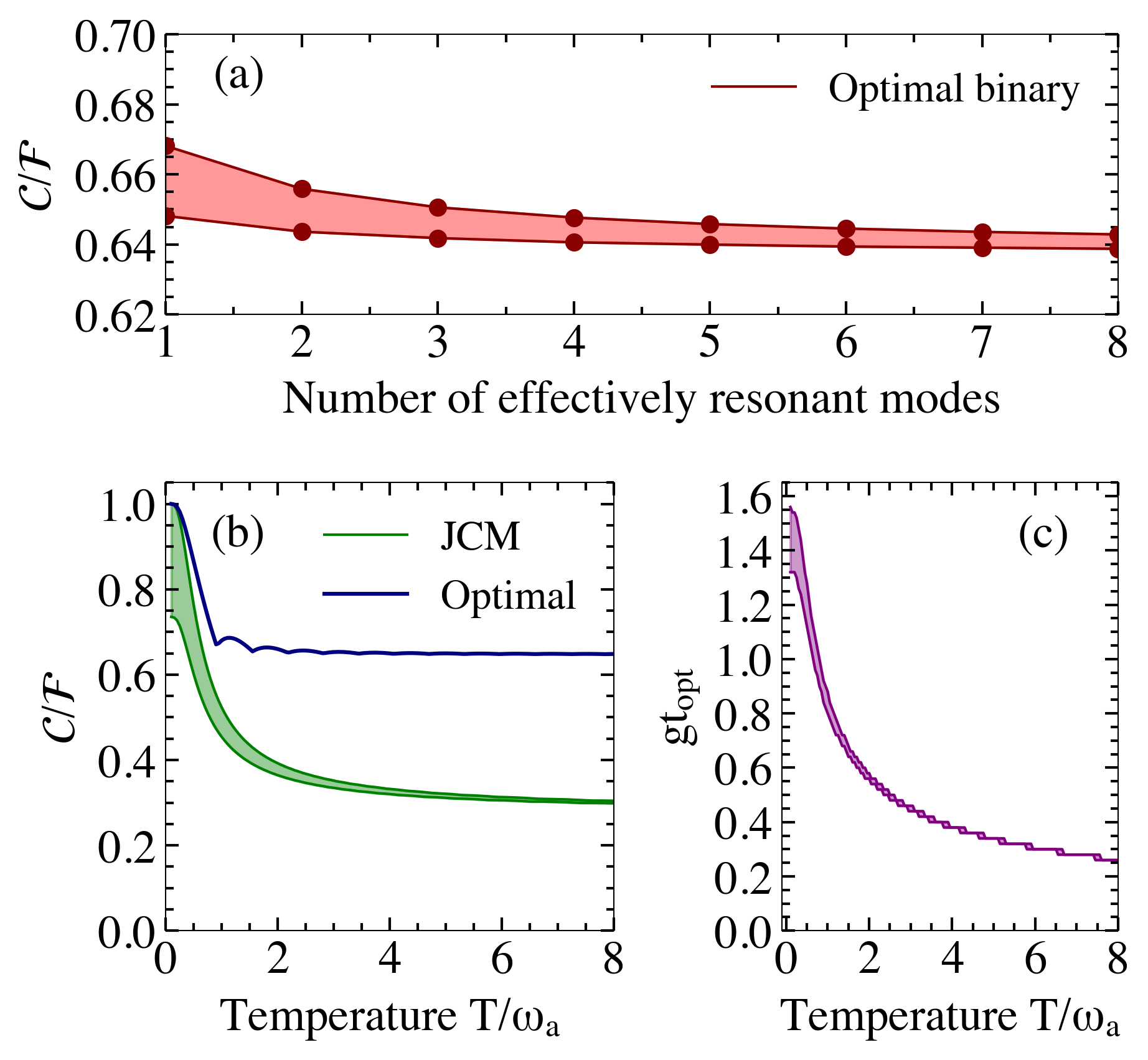
We can then ask the question of how well one can estimate the BEC temperature by measurements on the quantum dot probe. In Fig. 7(a) we plot the coarse-grained vs thermal Fisher information ratio for the optimal binary measurement within the effectively resonant subspace. The ratio is given as a function of the number of effectively resonant modes, which would be expected to increase in proportion to the width of the spectral density. From the figure we see that the ratio approaches a value of 0.64 as the number of modes increase. This provides an optimal value against which to compare specific binary measurement strategies. Interestingly we see that the obtained ratio agrees with the optimal ratio found for a binary measurement on a system described by a Gaussian density of states.

If we now consider the specific case where the effectively resonant subspace consist of a single phononic mode, and furthermore make a rotating wave approximation, the resulting system is modelled by the paradigmatic Jaynes-Cummings Hamiltonian Langford et al. 2017:

$$H=\omega_{d}\sigma^{\dagger}\sigma+\omega_{a}a^{\dagger}a+g\left(\sigma^{\dagger}a+\sigma a^{\dagger}\right),$$

(45)

where $a,a^{\dagger}$ are the creation and annihilation operators of the bosonic cavity mode, $g$ is the coupling strength, and $\sigma=|g\rangle\!\langle e|$ where the excited and ground states of the quantum dot are denoted by $|e\rangle$ and $|g\rangle$ respectively. Experimental work has shown how such models arise for specific thermometry protocols Sabin et al. 2014, and our results makes it possible to evaluate how close such a strategy is to being optimal.

Consider a measurement protocol in which the quantum dot is initialized in its ground state. The quantum dot then evolves jointly with the BEC for a time $t$, after which the probability of finding the quantum dot in its excited state is give by

$$\mathbb{P}_{e}(t)=\sum_{n=0}^{\infty}\frac{e^{-\beta\omega_{a}(n+1)}}{Z_{\beta}}\frac{g^{2}(n+1)}{\lambda_{n}^{2}}\sin^{2}\left(\lambda_{n}t\right),$$

(46)

where we have defined $\lambda_{n}=\sqrt{\delta^{2}/4+g^{2}(n+1)}$ in terms of the detuning $\delta=\omega_{d}-\omega_{a}$. From this probability we can compute the coarse-grained Fisher information, see also Brunelli et al. 2011. In Fig. 7(b) we show the ratio of the coarse-grained Fisher information computed from Eq. (46) and optimized over the measurement time at each temperature, with the thermal Fisher information of the phononic mode itself. Inspection of the results show that the probe-based measurement gives a Fisher information which never falls below 45% of the optimal binary measurement strategy. In Fig. 7(c) we plot the optimal measurement time as a function of temperature, and we observe an inverse relationship between the optimal measurement time and the temperature. Notice that as the temperature approach absolute zero, the optimal measurement time for zero detuning approach $\pi/2g$ in agreement with known results Brunelli et al. 2011.

It is interesting to note that similar considerations for the Fisher information have been obtained for temperature measurements of micromechanical resonators via a qubit probe, whose interaction can also be described by the Jaynes-Cummings (45) Brunelli et al. 2011; and more general interaction Hamiltonians, either dropping the rotating wave approximation or considering interactions far off resonance, have also been considered Brunelli et al. 2012; Higgins et al. 2013. In all such cases, our considerations provide upper bounds on the maximal precision estimation with a qubit probe, as shown in Fig. 7. Indeed, the strength of our bounds is that they apply to arbitrary nonequilibrium strategies.