Low-Complexity Angle-Domain MIMO NOMA System with partial channel state information for MmWave CommunicationsThanks: This work has been funded by IMT Atlantique, Lebanese University research fund program and the AZM association.
Abstract
In millimeter-wave communication, digital beamsteering (DBS), only based on the user direction, is a promising angle-domain multi-antenna technique to mitigate the severe path loss and multi-user interference, with low-complexity and partial channel state information (CSI). In this paper, we design a power-domain non-orthogonal multiple access (NOMA) scheme that enhances the DBS performance trading-off complexity, energy-consumption and capacity performance. In particular, we propose a user-clustering algorithm to pair users, based on a geometric-interference metric, so that the inter-user interference is reduced. Afterward, based on a fixed inter-cluster power allocation, we derive analytically a sub-optimal intra-cluster power allocation optimization problem to maximize the network throughput. To address the issue of partial CSI, we rewrite the aforementioned optimization problem, by relying only on the user direction. Performance evaluation of the proposed schemes is developed in rural environment, based on the New York University millimeter-wave simulator. The obtained results demonstrate that the proposed low-complexity NOMA-DBS schemes with either full- or partial-CSI achieve significant performance improvement over the classical DBS, in terms of spectral- and energy-efficiencies (up to bps/Hz rate gain for 45 users using the proposed scheme with partial CSI).
1 Introduction
To meet the exponential growth of data traffic, the new generation of cellular systems needs to achieve higher network capacity and better energy efficiency. This is done by exploiting new and innovative technologies such as massive multiple-input multiple-output (m-MIMO) system, non-orthogonal multiple access (NOMA) technique and millimeter-wave (mmWave) bands [1, 2, 3]. These technologies can be integrated together to further enhance the network capacity [4]. Indeed, the m-MIMO beamforming (BF), which enables high directional array, overcomes the tremendous path loss in mmWave wireless communications where enormous bandwidths are available. In addition, using superposition coding (SC) at the base station (BS) and successive interference cancellation (SIC) at the receiver side, power-domain NOMA (PD-NOMA) effectively improves the connectivity density by multiplexing user equipments (UEs) into transmission power domain [3].
Recently, numerous research studies on NOMA-based multiuser MIMO (NOMA-MIMO) system have been initiated to enhance the spectrum efficiency. For instance, system-level simulations are presented in [5] and show a clear superiority of NOMA over orthogonal multiple access (OMA) in terms of system throughput. Moreover, the authors in [6] analytically compares the performance of NOMA-MIMO with OMA-MIMO in terms of the sum-channel- and ergodic-sum-capacities, when multiple users exist in a cluster. The analytical proof also indicates the superiority of NOMA-MIMO.
The most important challenges of NOMA-MIMO system include overall system overhead, user clustering, power allocation and beamforming techniques. For multicast NOMA-MIMO, an iterative algorithm is proposed in [7] to find the BF vector and the power for each UE that solves the power minimization problem. In [8], a joint beamforming and power allocation scheme was proposed to maximize the sum-rate of a 2-user mmWave NOMA-MIMO system using an analog BF structure with a phased array. A spectrum and energy efficient mmWave transmission scheme that integrates NOMA with beamspace MIMO was first proposed in [9], in order to reduce the hardware complexity and energy consumption by using lens antennas. In [9], the authors designed a precoding scheme based on the principle of zero forcing (ZF) to reduce the inter-cluster interferences.
However, [7, 9, 8, 6] require full channel state information (CSI), which is difficult to perform at BS and brings high feedback overhead in case of a large array system. To address this issue, the authors in [10] implemented a random beamforming for a 2-user NOMA-MIMO cluster to avoid the requirement of full CSI at BS. The authors exploit the key feature of mmWave systems, i.e., the highly directional transmission. Thereby, they proposed a low-feedback mmWave NOMA-MIMO schemes with a fixed power allocation where the two UEs in the NOMA cluster located in the same sector are classified based on their distances from BS instead of their effective channel gains. In [11], the power allocation for a Rayleigh fading 2-user NOMA-MIMO system without beamforming was investigated as an ergodic capacity maximization under statistical CSI. A m-MIMO NOMA system with limited feedback is designed in [12], where the m-MIMO NOMA channel is splited into multiple single input single output (SISO) NOMA channels, by exploiting the spatial correlation matrices of users’ channels.
To reduce the BF implementation complexity and the channel overhead in m-MIMO systems, the authors in [13] have been investigated the digital beamsteering (DBS). This geometric beamformer, based on the UEs’ direction, steers a single beam toward each UE, using just digital phase shifters. Our previous works [14, 15, 16] show that DBS is an appealing beamformer in the sparse mmWave environment trading-off complexity, performance and channel feedback. This is done using the stochastic mmWave channel model, called NYUSIM [17] built on real measurements and developed by New York University. The spatial resolution to discriminate users depends on the beamwidth, i.e. the number of antennas. However, the implementation of a large number of antennas is difficult due to high power consumption and transceiver complexity. We propose to tackle the problem of congested cell where the number of users is close to the number of antennas. To do so, we boost the DBS performance, without adding any additional antenna, by implementing PD-NOMA, as an alternative and innovative solution. Moreover, we aim to maintain a low complexity, low overhead solution, by assuming partial CSI at the BS.
Specifically, the major contributions of this paper are summarized as follows:
- •
We design a NOMA-DBS scheme that enhances the DBS performance without adding additional antennas, and then offers affordable hardware complexity and energy consumption. This is performed by integrating DBS with the PD-NOMA transmission, by which more than one UE can be served by each beam. The aim of the proposed NOMA-DBS scheme is to boost the DBS performance by reducing the spatial inter-beam interference (IBI).
- •
We leverage the spatial behavior of DBS in mono- and multi-path environments, and then we define a geometric interference metric based on the UE’s direction. Accordingly, we propose a user clustering algorithm for 2-UE NOMA-DBS system based on the aforementioned geometric metric instead of the effective channel gain or the channel correlation as adopted in the literature, so that reduces spatial IBI based only on the UEs’ directions.
- •
Given the set of clusters, we aim at maximizing the system throughput under transmission power and SIC constraints. Accordingly, the corresponding optimal intra-beam power allocation method is achieved by assuming a fixed inter-beam power allocation. However, the obtained scheme requires full channel feedback.
- •
To tackle the system overhead issue, we define a partial CSI-based geometric function relying on the overall system throughput. Thereby, we reformulate a sub-optimal problem that maximizes the new geometric function, instead of the system throughput.
- •
By simulations, we verify the performance in terms of both spectrum and energy efficiencies of the proposed NOMA-DBS scheme with either full or partial channel feedback in rural environment, using NYUSIM.
The rest of this paper is organized as follows: Section 2 presents the model of the proposed NOMA-DBS scheme. In Section 3, we investigate the spatial behavior of DBS and propose a user clustering method. Section 4 and Section 5, respectively, discuss the proposed full and partial CSI-based intra-cluster power allocation schemes. Section 6 numerically evaluates the performance of the proposed schemes, while Section 7 concludes the paper.
Symbol Notations: A, a and denote matrix, vector and scalar, respectively. is a Gaussian random variable with mean and variance . , and stand for the transpose, the conjugate transpose and the trace, respectively.
2 Description of NOMA-DBS System
This study is conducted on a downlink 3 dimensions (3D) MU-MIMO system consisting of a BS equipped with a 2 dimensions (2D) array of antennas, where and are the number of horizontal and vertical antennas, respectively. The BS concurrently communicates with single-antenna UEs (), which are randomly distributed in the cell. Denote as the set of UEs. Based on the angle information of the UE’s direction and using digital phase shifters, classical DBS generates beams. Each beam only serves a single UE. Thus, with space division multiple access (SDMA) strategy implemented via DBS, all UEs exploit the whole system bandwidth for high data rate communication.
In a congested cell, where the number of users is close to the number of antennas, the main problem of DBS is IBI, that impacts drastically the system performance in terms of sum-rate. To tackle this issue, we design a NOMA-DBS system, as illustrated in Fig. 1. In the proposed scheme, UEs located at the same direction are allowed to be served by one beam and the BS communicates with them by exploiting the PD-NOMA transmission protocol.
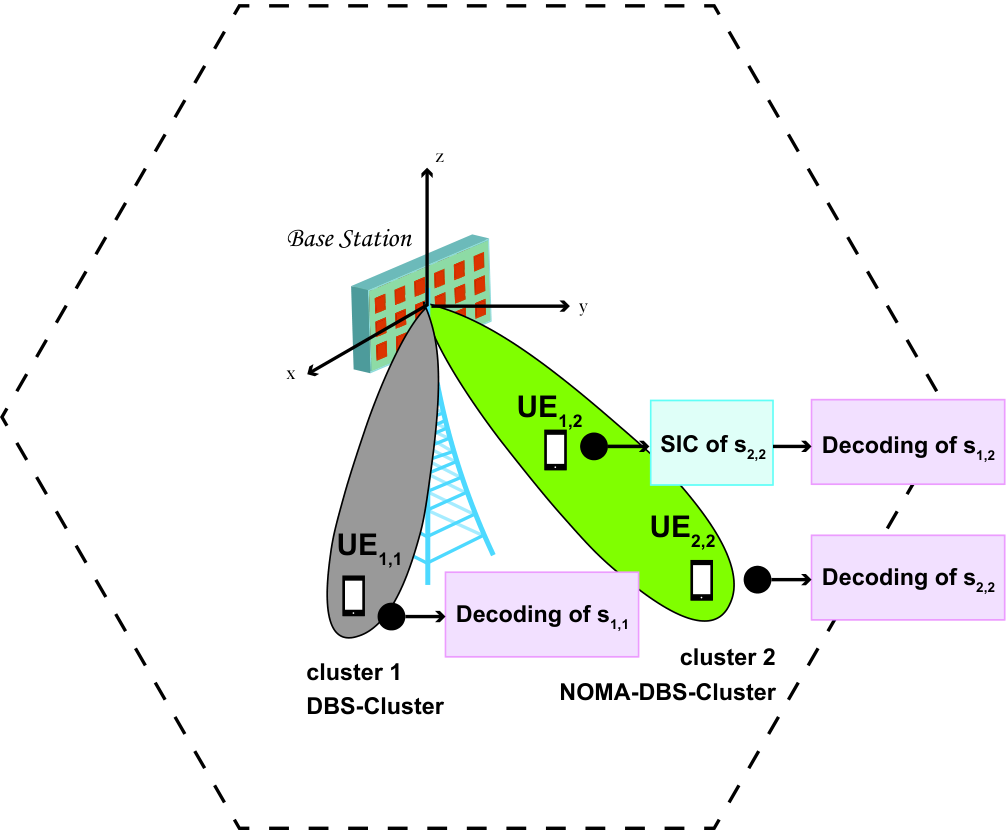
Consequently, two different types of cluster exist, namely DBS-cluster and NOMA-DBS-cluster as depicted in Fig. 1. In the former cluster, only one UE is served using classical DBS. However, in the latter, multiple UEs are served by the same beam and share the same time-frequency resources using PD-NOMA. Now, the UEs are served simultaneously by beams (or clusters).
2.1 System model
Let and be the number of DBS- and NOMA-DBS-clusters, respectively and be the number of UEs in the th cluster. Hence, . Denote and as the set of DBS- and NOMA-DBS-clusters, respectively, as the set of all clusters and as the set of UEs in the th cluster.
Based on available CSI and user clustering, detailed in section 3, the BS multiplexes UEs in the power domain using SC, so as to transmit the signals of UEs grouped in the same cluster within the same beam. Thus, BS constructs the superimposed signal , given by:
| (1) |
where is the modulated complex symbol corresponding to the th UE in the th cluster, denoted as UE, is the power allocated to the th cluster, and is the power allocation coefficient for , such that .
Moreover, according to DBS, the BS steers a beam toward each cluster in both azimuth and elevation domains. This implies that the transmit BF matrix is defined as with , the BF weight vector corresponding to the th cluster. is the array steering vector corresponding to the direction of the th cluster, with the azimuth angle and the elevation angle. In this study, we conduct a 3D MIMO channel with uniform planar array (UPA) located in plane, as shown in Fig. 1. Therefore, the antenna array steering vector is a function of and with:
| (2) |
| (3) |
where is the antenna spacing and is the wavelength.
Then, the signal transmitted from BS can be expressed as:
| (4) |
where is the normalization factor that eliminates the beamforming effect on the transmission power. Thus, the received signal is expressed as:
| (5) |
where is the additive white Gaussian noise, and is the multi-path 3D channel vector between BS and UEl,c, which is given by:
| (6) |
where is the number of multi-path components in UEl,c’s channel, is the complex gain and is the departure angle of the th path in UEl,c’s channel, respectively. Denote as the index of the line-of-sight (LOS) path, i.e., the strongest path generated by NYUSIM.
2.2 System model with SIC
In the rest of the study, we consider only 2 UEs per NOMA-DBS cluster, such that , to limit the complexity of SIC at the receiver. The number of UEs per DBS-cluster is equal to 1.
For DBS-cluster and 2-UE NOMA-DBS-cluster, the direction of the th cluster used to form the beams is calculated as follows:
| (7) |
Thus, only the departure angle of the LOS path () is considered.
Based on the user clustering method and the set of instantaneous received power at all UEs, the two UEs regrouped in each NOMA-DBS cluster are classified between strong and weak UEs according to the descending order of their received power, i.e., . Moreover, SIC applied at strong UE, denoted as UE1,c will work properly if the power allocation coefficients satisfy the following condition as mentioned in [18]:
| (8) |
where is the minimum power difference. In fact, (8) maintains the power difference between strong and weak UEs’ signals, so that SIC at strong UE’s receiver can decode first the data of the weak UE, and then subtract it from the superimposed signal to decode his own signal. However, NOMA-DBS system also suffers from the inter-cluster interference unlike the classical PD-NOMA in [18]. Therefore, we propose to take into account the interference from the other clusters and (8) will be given by:
| (9) |
where is the interference at UEl,c from all other clusters. From (9), we find that the transmit power of UE2,c must be larger than that of UE1,c, thus satisfying the PD-NOMA transmission protocol.
According to PD-NOMA principle, UE1,c in NOMA-DBS cluster conducts SIC to eliminate the intra-cluster interference from UE2,c. We assume a perfect SIC at the receiver side of UE1,c. In other words, the interference at UE1,c from UE2,c, denoted as , is totally eliminated, i.e., . Therefore, the received signal at UE1,c after SIC can be expressed as:
| (10) |
And, the signal-to-interference-plus-noise ratio (SINR) of UE1,c in NOMA-DBS cluster is given by:
| (11) |
However, UE2,c of NOMA-DBS cluster treats the UE1,c signal as an interference and the received signal at UE2,c can be expressed as:
| (12) |
Therefore, the SINR of UE2,c is given by:
| (13) |
For DBS-cluster, the received signal and are also calculated as in (10) and (11), respectively, with .
The SINR achieved at UEl,c in DBS and NOMA-DBS clusters can be rewritten as:
| (14) |
| (15) |
| (16) |
where
| (17) |
| (18) |
| (19) |
As seen in (5), represents the received power at UEl,c of the superimposed signal, that is transmitted in the th cluster. And, represents the interference at UEl,c coming from the other clusters plus the noise power. This implies that is the superimposed-signal to other-clusters interference plus noise ratio at UEl,c, which is different than SINRl,c for NOMA-DBS cluster and represents SINR1,c for DBS-cluster. Therefore, (9) can be simplified as follows:
| (20) |
3 3D Geometric Interference Metric and User Clustering Method (-UC)
In this section, we discuss the factors affecting the interference level at each UE in case of classical DBS, in both mono- and multi-path environments, to define later a 3D geometric interference metric. Subsequently, we propose a user clustering strategy based on the aforementioned metric.
3.1 Classical DBS Performance
In case of classical DBS, we use the subscript instead of .
3.1.1 Mono-path environment
In mono-path environment, the SINR achieved using DBS at UEk is given by [15]:
| (21) |
where is the steering vector corresponding to the LOS path angle of UEk, denoted as , is the complex gain of the LOS path in UEk’s channel, and is the normalization factor when BS adopts only DBS.
For classical DBS in mono-path environment, the interference term at UEk, observed at the denominator in (21), only depends on , i.e., the spatial interference causing by the beam generated for UEu with the LOS path in the UEk’s channel. In other words, if UEk and UEu are located at the same direction, i.e., is closed to , then DBS system suffers from high IBI, and thus the DBS performance degrades.
3.1.2 Multi-path environment
Similarly, in multi-path environment, DBS also generates a single beam in the LOS path direction. Therefore, is given by [15]:
| (22) |
where , and are complex gain, angle and steering vector of the th path in UEk’s channel, respectively.
As seen in (22), the interference at UEk is caused by the LOS beam of UEu (), represented by , that interferes with all paths of UEk, represented by . Thus, the interference results from both non-LOS (NLOS) and LOS paths. However, DBS is a geometric beamformer, that doesn’t exploit the NLOS paths and generates a single beam in the LOS path direction, i.e., the directions of the UEs. This simplifying assumption makes possible partial CSI and feedback solely based on the UEs’ directions but restricts the sum rate, since all the path diversity is not exploited.
3.2 Interference Metric
To enhance the DBS performance, our proposed NOMA-DBS scheme divides UEs into clusters based on their spatial direction, which directly reflects in their spatial interferences.
Based on the simplifying assumption and the previous analysis in Section 3.1, we define as a 3D geometric metric representing the normalized spatial interference at UEk from the beam generated for UEu, and vice versa. Applying (2) and (3), using UPA, is given by:
| (23a) | ||||
| (23b) | ||||
| . | ||||
According to (23), , and represents the value of the normalized array pattern [19] of the beam pointed at UEu direction for , i.e.,
| (24) |
Remark 1
Based on (24), we can see that if the angular distance , i.e., , then . Thus, the smaller and are, i.e., UEk and UEu are closely at the same direction in azimuth and elevation domains, the larger is.
Remark 2
gives a measure of the 3dB-beamwidth expressed in terms of the azimuth and elevation widths of the beam generated at UEu, which depend on the beam direction and the number of horizontal and vertical antennas. and are defined as the angular distances that satisfy . This implies that implicitly provides information regarding the beamwidth .
Therefore, we define the interference threshold , such that means that the LOS path of UEk lies in the UEu beam in both azimuth and elevation domains. Particularly, the -beamwidth defines the azimuth and elevation angular distances satisfying . Thus, is an important metric to determine the level of spatial interference based on a geometric partial channel knowledge, namely the UE direction, i.e., ().
3.3 User clustering algorithm
We would like to apply NOMA to UEs that produce high spatial interference to each other, whereas the others are treated via DBS. To perform user clustering, we take profit of the 3D geometric interference based on the angles of the LOS path of each user. To the best of our knowledge, it is the first time that such a geometric metric is used in user clustering. The main idea of our proposed UC, denoted as -UC, is to regroup two-by-two UEs (UEu and UEk) with large inter-beam interference, i.e., , into the same cluster, whose beam angle is defined in 7. Subsequently, we assign a single cluster to the remaining UEs with cluster angle equal to their LOS path angle, as mentioned in (7). The proposed -UC algorithm can be given as in Algorithm 1.
.
.
.
.
4 Full CSI-based Power Allocation Scheme
In this section, we design a power allocation (PA) scheme based on full CSI, that maximizes the throughput of the NOMA-DBS system. However, DBS is a geometric beamformer that requires only the UE’s direction. For that, it’s more significant to design a PA scheme based on partial CSI, which is presented in Section 5.
4.1 Problem Formulation
The system throughput, which is defined as the maximum quantity of the transmitted information over the NOMA-DBS system, is given by a sum of the UEs’ data rates:
| (25a) | ||||
| (25b) | ||||
where [] is the achievable data rate for UEl,c and can be expressed, according to Shannon formula, as:
| (26) |
Therefore, can be defined as a function of the inter-cluster PA and the intra-cluster PA , since , i.e., :
| (27) |
where is the throughput of UEs grouped in DBS-clusters, is the throughput of strong UEs grouped in NOMA-DBS-clusters and is the throughput of weak UEs grouped in NOMA-DBS-clusters. Using (14), (15) and (16), , and are given by (28), (29) and (30), respectively:
| (28) |
| (29) |
| (30) |
The aim of the proposed PA scheme is to maximize the sum of the UEs’ data rates over the NOMA-DBS system. Therefore, the corresponding optimization problem denoted by is formulated as follows:
| (31) | ||||
must be done under the power allocation constraints and and the SIC constraint obtained in (20).
Problem maximizes the system throughput by jointly optimizing intra- and inter-cluster PA. However, because the coupling of the power allocation factors from different UEs, then it is difficult to obtain the optimal solutions. To this end, we add a constraint that addresses this issue and then simplifies by applying a fixed inter-cluster PA. Thus once -UC is applied, the power allocated to each cluster will be well known and equal to constant values as detailed in Section 4.2. Hence, can be reformulated as follows:
| (32) | ||||
For DBS cluster, as seen in (28), the throughput of UEs grouped in DBS-cluster is the same regardless of the intra-cluster PA method, i.e., (). However, for NOMA-DBS cluster, as seen in (29) and (30), the data rates of UE1,c and UE2,c only depend on their PA coefficients and . To this end, based on -UC, the PA scheme maximizing the system throughput is equivalent to that maximizing the throughput of each NOMA-DBS cluster separately. Accordingly, the maximization problem can be seen as an equivalent problem of independent optimization problems denoted by for the NOMA-DBS cluster, and can be equivalently formulated as follows:
| (33) | ||||
and in problem (31) can be reformulated as . Moreover, , and specify the feasible interval of , that is with:
| (34) |
4.2 Fixed Inter-Cluster Power Allocation
In our previous work [16], we applied a uniform power allocation per cluster, i.e., . We define the emitted power toward the th cluster as follows:
| (35) |
Moreover, where is the total transmit power. This implies that the uniform power allocation per cluster satisfies , using . However, in this study, we allocate a power to the th cluster proportional to the number of UEs served in the th cluster. Accordingly, based on (35), is also proportional to . This is supposed to guarantee the power fairness among UEs. Therefore, we calculate as follows:
| (36) |
From (35) and (36) we obtain that:
| (37) |
4.3 Intra-Cluster Power Allocation Solution with Full CSI
In this subsection, we propose an intra-cluster PA scheme, for the problem for each NOMA-DBS cluster, denoted as OPA, which is summarized in Algorithm 2.
while do
Lemma 1
is a real monotone function of , and its variation depends on the sign of .
Proof 1
See Appendix 1.
From Lemma 1, is a real monotone function of , and its variation is as follows:
| (38) |
For the three cases, and since UE1,c is the strong UE, i.e., , this implies that . If , then . And, UE1,c taken as a strong UE suffers from high other-clusters interference compared to UE2,c. This implies that even though UE1,c has the highest received superimposed signal, the level of interference at each UE from other clusters determines the variation of the function .
From Lemma 1 and based on the derivation and analysis in Section 4.3, the optimal solution of Problem is achieved at the end point of the feasible interval of . Indeed, if , i.e., is an increasing function, then . The authors in [18] propose an optimal PA policy that maximizes the sum-throughput of a classical NOMA system (NOMA-SISO) by maximizing the sum-throughput per m-user NOMA cluster (). Using Karush-Kuhn-Tucker optimality conditions, they derived the optimal PA. We find that for 2-UE NOMA-SISO cluster (see Table 1 [18]), the optimal PA can be similar to our solution obtained without using Lagrange, by changing variables. Otherwise, if , i.e., is a decreasing function, then . This implies that OPA deactivates UE1,c, which is classified as strong UE, but actually suffers from high inter-cluster interference, by allocating all the power to UE2,c. In addition, when , each value belonging to the interval of can be taken as an optimal solution. But, we choose that achieves fairness between UEs in the th cluster, i.e., , thus with
| (39) |
Lemma 2
When is a constant function, then chosen as the optimal solution of Problem satisfies the power allocation constraint .
Proof 2
As seen in (38), is a constant function if . Therefore, for , can be expressed as:
| (40) |
Applying the first-order derivative of (40), we obtain that:
| (41) |
From (41), we find that for , and thus in (40) is a decreasing function. This implies that if , then .
| (42) |
Accordingly, based on (42), lies on for . Here, Lemma 2 is proved.
Remark 3
When is a slowly-increasing or slowly-decreasing function, the absolute difference between at and at is very small, i.e., . However, since , then is also valid in the feasible interval of , i.e., . Therefore, we use instead of , which is more complicated to compute. Moreover, the value of depends on the value of . To this end, we use the relative difference of the corresponding data rates instead of .
5 Partial CSI-based Power Allocation Scheme
Using classical DBS, UEs only feedback their estimated angles, i.e., . Accordingly, we design a NOMA-DBS scheme that uses these angles to schedule UEs between DBS and NOMA-DBS clusters. Subsequently, in Section 4, we propose an intra-cluster PA scheme for NOMA-DBS, denoted as OPA, that maximizes the system throughput under full CSI. This implies that NOMA-DBS misses the key features of DBS, namely partial CSI and low channel overhead. To this end, we will formulate an alternative problem from , by defining a partial CSI-based function, to guarantee low feedback overhead. First, we will try to rewrite of UEl,c served in NOMA-DBS cluster, by exploiting the impacts of the NLOS and LOS paths on both received power and interference at UEl,c. Then, we will rewrite the system throughput to conclude a partial CSI-based geometric function.
Based on (6), can be expressed as:
| (43a) | ||||
| (43b) | ||||
In (43b), the first term represents the spatial interference of the th cluster with the LOS path in UEl,c’s channel. And, the second term represents the spatial interference of the th cluster, with all the NLOS paths in UEl,c’s channel.
In high signal-to-noise ratio (SNR) regime and using (43), in (11) and in (13) are given by (44) and (45), respectively:
| (44) |
| (45) |
As seen in (44) and (45), the NLOS paths affect either the received power or the interference. Indeed, the interference is due to the beams of other UEs that interferes with LOS and NLOS paths. In addition, the received power at UEl,c is that transmitted by the beam interfered with the LOS path plus the effect of paths in the vicinity of the beam direction.
Assuming that this NLOS paths’ impact is negligible, i.e., is negligible, thus the data rates at UEl,c can be approximated as follows:
| (46) |
| (47) |
As seen in (46) and (47), depends on the LOS path angle information, i.e., , the -UC, i.e., , and the applied PA method, i.e., and . The obtained partial CSI-based function corresponds to the data rate at UEl,c in case of mono-path environment, where the received power just comes from the LOS path and the interference comes from the other-clusters with the LOS path. However, DBS is a LOS path angle-based beamformer that generates a single beam toward each UE. Thus, in multi-path environment, DBS loses the potentiality of the NLOS paths and some of the radiated energy, as obtained in [15]. To guarantee the key feature of DBS, we formulate a partial CSI-based function that misses the potentiality of the NLOS paths. Accordingly, the problem from consists to find the PA coefficients that maximize the partial CSI function instead of the NOMA-DBS cluster’s throughput , as follows:
| (48) | ||||
This Problem will be solved in the same manner as Problem , but with , where:
| (49) |
| (50) |
6 Performance Evaluation
In this section, numerical results are presented to verify the performance of the proposed NOMA-DBS scheme. All results are obtained by averaging over random trials. Perfect estimation of angles at the receivers and perfect instantaneous feedback of the estimated angles are assumed in the analysis of such systems. We set as the spatial interference threshold. Other system and channel parameters used for performance assessment are listed in Table 1.
| System and Channel Parameters | Values |
|---|---|
| Number of transmit antennas | 64 |
| Carrier frequency | 28 GHz |
| Channel bandwidth | 20 MHz |
| Cell edge radius | 100 m |
| Transmission power | 30 dBm |
| Noise power | -100.9178 dBm |
| Minimum power difference | 1 mW |
| Number of paths per time cluster in rural scenario |
The proposed schemes with full and partial CSI are labeled, respectively, as "-UC NOMA-DBS-FCSI" and "-UC NOMA-DBS-PCSI". For comparison, the orthogonal multiple access (OMA) with DBS (OMA-DBS) is adopted as the baseline, in which the two UEs in NOMA-DBS cluster obtained using -UC algorithm are served using OMA with equal degrees of freedom for each UE, which is labeled as "-UC OMA-DBS". Moreover, a widely used beamformer, namely maximum rate ratio, also known as conjugate beamforming (CB) [20] is adopted to make a comparison. The number of real coefficients needed per channel estimation for the different systems is summarized in Table 2.
| System | Number of real coefficients per channel estimation for each UE |
|---|---|
| Classical DBS | 2 |
| MRT | [H] |
| -UC NOMA-DBS-FCSI | [] |
| -UC NOMA-DBS-PCSI | 3 [ + ] |
| -UC OMA-DB | [H] |
6.1 Spectral Efficiency
Fig. 2 depicts the spectral efficiency (or the achievable sum-rate per the normalized bandwidth) versus the total number of users, in rural environment, when BS is equipped using UPA with .

It can be seen that the proposed NOMA-DBS scheme with full and partial CSI significantly improves the performance of classical DBS. Fortunately, attractive results are achieved, where NOMA-DBS-PCSI can almost achieve the same performance as NOMA-DBS-FCSI, with much lower channel feedback; times less as indicated in Table 2. Indeed, one or two paths exist in rural environment (see Table 1), and thus the partial CSI-based function in NOMA-DBS-PCSI scheme is approximately the same as the throughput. For instance, NOMA-DBS-PCSI achieves higher spectral efficiency with respect to DBS up to for 45 users in the cell using UPA.
As seen in Fig. 2, it is obvious that classical DBS outperforms CB in rural environment, thanks to a few paths as explained in our previous work [15]. Besides, NOMA-DBS improves the performance of DBS and thus surpasses CB. For instance, the performance gain in spectral efficiency for NOMA-DBS-PCSI against CB is approximately for 45 users in the cell using UPA, with lower complexity and much lower channel overhead ( times less as shown in Table 2).
It can be seen from Fig. 2 that NOMA-DBS surpasses the conventional OMA-DBS schemes in rural environment, and using UPA. This is also obtained in the prior work comparing NOMA-MIMO with OMA-MIMO, which concludes that OMA-MIMO can not support more users, while NOMA-MIMO enables a higher number of successfully connected users. Indeed, NOMA with the aid of SIC and SC enables more UEs in each beam to be supported at the same spectrum efficiency, while OMA serves only one UE in each beam.
6.2 Energy Efficiency
The energy efficiency (EE) is also a key performance metric used for future cellular network, because of environmental and economic interests. EE is defined as the ratio of the spectral efficiency to the total power consumed at BS:
| (51) |
where is a constant modeling the inefficiency of the power amplifier, is the constant power consumption per antenna independent of the transmitted power, and is the basic power consumed at the base station independent of the number of antennas. Assume , and .


Fig. 3 and 4 depict, respectively, the spectral efficiency and energy efficiency versus number of users, for NOMA-DBS using UPA with and , and for classical DBS using UPA with and different values of () in rural environment.
In rural environment, using less of antennas, our proposed schemes NOMA-DBS-FCSI and NOMA-DBS-PCSI with and have almost the same performance of the classical DBS with and in terms of spectrum efficiency, as shown in Fig. 3. It’s obvious therefore that the energy efficiency using NOMA-DBS is times greater than that using classical DBS with and , as seen in Fig. 4. Accordingly, NOMA-DBS is an alternative solution to enhance the DBS performance without increasing the number of antennas.
7 Conclusion
In this paper, we integrate DBS with PD-NOMA transmission for mmWave massive MIMO systems in order to boost the DBS performance without increasing the number of antennas. We first define a geometric interference metric, so that the proposed NOMA-DBS scheme regrouped the users based on their directions. Subsequently, by applying a fixed inter-cluster PA, we derive an intra-cluster PA for 2-user NOMA-DBS system that maximizes the sum-throughput. More importantly, a new partial CSI-based geometric function is defined by exploiting the spatial behavior of DBS, to design a PA scheme with low-feedback rate. Simulation results using NYUSIM indicates that our proposed low-complex NOMA-DBS system with limited feedback yields a significant spectral efficiency improvements with respect to DBS, and can be an alternative solution to the use of a large number of antennas. However, our proposed scheme is limited to 2-user in NOMA-DBS cluster. It is in our interest to extend 2-user NOMA-DBS to support multiple users, to further enhance the NOMA-DBS scheme.
8 Appendix
8.1 Appendix 1
References
- [1] Busari, S.A., Huq, K.M.S., Mumtaz, S., Dai, L., Rodriguez, J.: ‘Millimeter-wave massive MIMO communication for future wireless systems: A survey’, IEEE Communications Surveys & Tutorials, 2017, 20, (2), pp. 836–869
- [2] Araújo, D.C., Maksymyuk, T., de Almeida, A.L., Maciel, T., Mota, J.C., Jo, M.: ‘Massive MIMO: survey and future research topics’, IET Communications, 2016, 10, (15), pp. 1938–1946
- [3] Dai, L., Wang, B., Yuan, Y., Han, S., Chih.Lin, I., Wang, Z.: ‘Non-orthogonal multiple access for 5G: solutions, challenges, opportunities, and future research trends’, IEEE Commun Mag, 2015, 53, (9), pp. 74–81
- [4] Zhang, D., Zhou, Z., Xu, C., Zhang, Y., Rodriguez, J., Sato, T.: ‘Capacity analysis of NOMA with mmWave massive MIMO systems’, IEEE J Sel Areas Commun, 2017, 35, (7), pp. 1606–1618
- [5] Benjebbovu, A., Li, A., Saito, Y., Kishiyama, Y., Harada, A., Nakamura, T. ‘System-level performance of downlink NOMA for future LTE enhancements’. In: Proc. IEEE Globecom Workshops (GC Wkshps). (IEEE, 2013. pp. 66–70
- [6] Zeng, M., Yadav, A., Dobre, O.A., Tsiropoulos, G.I., Poor, H.V.: ‘Capacity comparison between MIMO-NOMA and MIMO-OMA with multiple users in a cluster’, IEEE J Sel Areas in Commun, 2017, 35, (10), pp. 2413–2424
- [7] Choi, J.: ‘Minimum power multicast beamforming with superposition coding for multiresolution broadcast and application to NOMA systems’, IEEE Transactions on Communications, 2015, 63, (3), pp. 791–800
- [8] Xiao, Z., Zhu, L., Choi, J., Xia, P., Xia, X.G.: ‘Joint power allocation and beamforming for non-orthogonal multiple access (NOMA) in 5G millimeter wave communications’, IEEE Transactions on Wireless Communications, 2018, 17, (5), pp. 2961–2974
- [9] Wang, B., Dai, L., Wang, Z., Ge, N., Zhou, S.: ‘Spectrum and energy-efficient beamspace MIMO-NOMA for millimeter-wave communications using lens antenna array’, IEEE Journal on Selected Areas in Communications, 2017, 35, (10), pp. 2370–2382
- [10] Ding, Z., Fan, P., Poor, H.V.: ‘Random beamforming in millimeter-wave NOMA networks’, IEEE access, 2017, 5, pp. 7667–7681
- [11] Sun, Q., Han, S., Chin.Lin, I., Pan, Z.: ‘On the ergodic capacity of MIMO NOMA systems’, IEEE Wireless Communications Letters, 2015, 4, (4), pp. 405–408
- [12] Ding, Z., Poor, H.V.: ‘Design of massive-MIMO-NOMA with limited feedback’, IEEE Signal Process Lett, 2016, 23, (5), pp. 629–633
- [13] Rozé, A., Hélard, M., Crussière, M., Langlais, C. ‘Millimeter-wave digital beamsteering in highly line-of-sight environments for massive MIMO systems’. In: Wireless World Research Forum Meeting. vol. 35. (, 2015.
- [14] Khaled, I., EL Falou, A., Langlais, C., ELHassan, B., Jezequel, M. ‘Performance evaluation of linear precoding mmwave multi-user MIMO systems with NYUSIM channel simulator’. In: Proc. IEEE Middle East and North Africa COMMunications Conference (MENACOMM). (IEEE, 2019. pp. 1–6
- [15] Khaled, I., El Falou, A., Langlais, C., ELHassan, B., Jezequel, M. ‘Multi-user digital beamforming based on path angle information for mm-Wave MIMO systems’. In: Proc. International ITG Workshop on Smart Antennas (WSA). (VDE, 2020. pp. 1–6
- [16] Khaled, I., Langlais, C., El.Falou, A., Jezequel, M., ElHasssan, B. ‘Joint SDMA and power-domain NOMA system for multi-user mm-Wave communications’. In: Proc. International Wireless Communications and Mobile Computing (IWCMC). (IEEE, 2020. pp. 1112–1117
- [17] Samimi, M.K., Rappaport, T.S.: ‘3-D millimeter-wave statistical channel model for 5G wireless system design’, IEEE Trans Microw Theory Tech, 2016, 64, (7), pp. 2207–2225
- [18] Ali, M.S., Tabassum, H., Hossain, E.: ‘Dynamic user clustering and power allocation for uplink and downlink non-orthogonal multiple access (NOMA) systems’, IEEE access, 2016, 4, pp. 6325–6343
- [19] Hansen, R.C.: ‘Phased array antennas’. vol. 213. (John Wiley & Sons, 2009)
- [20] Yang, H., Marzetta, T.L.: ‘Performance of conjugate and zero-forcing beamforming in large-scale antenna systems’, IEEE J Sel Areas Commun, 2013, 31, (2), pp. 172–179