Primordial monopolium as dark matter
Abstract
The existence of monopoles is a characteristic signature of Kaluza-Klein multidimensional theories. The topology of these solutions is extremely interesting. The existence of a dipole solution, which we have associated to a monople-anti-monopole bound state, is the leitmotiv of this investigation. The dipole in its lowest energy state, which we here call also monopolium, is electromagnetically inert in free space interacting only gravitationally. Monopolium when interacting with time dependent magnetic fields acquires a time dependent induced magnetic moment and radiates. We have analyzed the most favorable astrophysical scenario for radiative monopolium and found that the amount of radiation is so small that is not detectable by conventional equipments. These findings suggest that Kaluza-Klein monopolium, if existent, would be a candidate for a primordial dark matter constituent.
pacs
04.20.Jb, 04.50+h, 04.50Gh,04.80-yI introduction
The nature of dark matter is one of the most relevant problems of physics today. Cosmological experiments have determined its abundance Aghanim:2018eyx. From observational and numerical simulations we have some knowledge about its distribution in galactic halos Wechsler:2018pic. Still the nature of dark matter remains unknown. Since the favorite explanations in the past, the weakly interacting particles, have eluded detection it is worthwhile to consider other possibilities.
Monopole physics took a dramatic turn when ’t Hooft 'tHooft:1974qc and Polyakov Polyakov:1974ek independently discovered that the SO(3) Georgi-Glashow model Georgi:1972cj inevitably contains monopole solutions. These topological monopoles appear naturally in Grand Unified Theories and are impossible to create in present day particle colliders because of their huge GUT mass Preskill:1984gd; Shnir:2005xx and they are very rear in the universe since inflation reduces their density dramatically Guth:1980zm; Linde:1981mu. ’t Hooft-Polyakov monopoles cannot built up dark matter because of their incredibly strong interactions Dirac:1948um.
It has been a long time since Kaluza and Klein first investigated the idea of unification of gravitation and gauge theories by exploring the possibility that the number of spacetime dimensions is greater than four Kaluza:1984ws; Klein:1926tv. The idea behind Kaluza-Klein (KK) theories is that the world has more than three spatial dimensions and some of them are curled up to form a circle so small as to be unobservable. KK theories have been the subject of revived interest in recent years since many standard model extensions in extra dimensions yield KK theories. KK theories contain a very rich topological structure, which includes very heavy monopoles whose mass is of the order of the Planck mass Gross:1983hb; Sorkin:1983ns; Newman:1963yy; Hawking:1976jb; Gibbons:1979xm. But most important for the present study, they also contain other soliton solutions in different topological sectors. In particular, the dipole, which has the quantum numbers of a monopole-anti-monopole bound state. This state in conventional gauge theories was called monopolium Hill:1982iq; Vento:2007vy; Epele:2007ic, and we kept the name here. In conventional gauge theories monopolium has vacuum quantum numbers and annihilates into more elementary constituents. However, in KK theories monopolium does not belong to the topological sector of the vacuum and therefore it is classically stable Gross:1983hb; Kerr:1963ud; Gibbons:1976ue. That solitons of KK theories could supply dark matter has been briefly discussed in the past Overduin:1998pn. The aim of this paper is to show that monopolium, as it appears in KK theories, if it survives inflation in sufficient numbers, could be a candidate for a primordial constituent of dark matter, and thus its study would open a window into the physics of more than four dimensions.
The presentation is based on the scenario discussed by Gross, Perry and Sorkin (GPS) Gross:1983hb; Sorkin:1983ns, which serves as a toy model, but our results are based on properties which arise in realistic scenarios. Let us describe them precisely. A topology where the dipole does not have vacuum quantum numbers Newman:1963yy; Hawking:1976jb; Gibbons:1979xm; Kerr:1963ud; Gibbons:1976ue. The dipole structure, described in terms of some parameter (distance between center of the poles), approaches the monopole-anti-monopole structure as becomes large. This also occurs in topological schemes with different topological sectors like in the Skyrme Model Zahed:1986qz. The dipole can thus be interpreted as a bound state with a mass smaller than twice the monopole mass. The parameter describes the magnetic moment of the dipole. The ground state (smallest mass) dipole, i.e. when , has vanishingly small dipole moment and therefore it is electromagnetically neutral and thus has only gravitational interaction. The GPS model has all these ingredients and therefore we are going to use it as a toy model to develop the ideas and get orders of magnitude for observables. However, the GPS model has a peculiar way of realizing the equivalence principle, which we will discuss in some detail, and we will show one mechanism for avoiding it.
In section II we are going to recall some aspects of the topology of the Kaluza-Klein theory in particular the existence of monopoles and dipoles. In section III we analyze if the dipole survives the inflationary process. In section IV we look for possible electromagnetic observables of monopolium and in section V we discuss possible experimental observations. Their size allows us to propose monopolium as a dark matter component. We end by some concluding remarks.
II Kaluza-Klein monopolium
Kaluza-Klein theories Kaluza:1984ws; Klein:1926tv contain topological solitons which can be identified as magnetic monopoles satisfying the Dirac quantization condition, Dirac:1948um. We next recall the structure of the KK monopoles by whose features can be extended to models with more compact dimensions Ezawa:1983gp; Bais:1984xb; Lee:1984ica; Xu:1988zj; Mann:2005gk; Cotaescu:2005jg.
The simplest topological solution in the GPS model is a magnetic monopole which arises from the generalization to more dimensions of the Taub-NUT solitonic solution Newman:1963yy; Hawking:1976jb and is described by the following metric
| (1) |
where and the spherical coordinates. At large distances the gauge field from the GPS solution behaves as a Dirac monopole Dirac:1948um
| (2) |
whose inertial mass is,
| (3) |
where is Planck’s mass and the fine structure constant. Note the non-perturbative character of this result in the inverse dependence on the structure constant.
These KK monopoles have a characteristic, which distinguishes them from all other types of monopoles, that makes them interesting and is the leitmotiv of the present investigation. In ordinary Yang-Mills theories one does not find solitons which are stable magnetic dipoles because the superposition of a monopole and an anti-monopole has the topology of the vacuum and therefore nothing prevents them from annihilating. The situation is quite different in KK theories. The vacuum solution belongs to a different topological sector than the monopole-anti-monopole solution Gibbons:1979xm. Since one cannot evolve smoothly from one type of solution to the other the monopole-anti-monopole pair will not annihilate classically. In the GPS scenario, KK dipoles can be constructed by the Kerr-Schwarzschild metric, which are regular solutions in euclidean dimensions, by compactifying the fourth dimension Gross:1983hb. This provides a very interesting topological state which has no magnetic charge and behaves like a magnetic dipole at large distances
| (4) |

where is the dipole mass and measures the distance between the poles. For large this solution coincides with the product ansatz of the monopole-antimonopole solution.
The mass of this dipole state is determined by the following equation,
| (5) |
where we use the Planckian System of untits . As can be seen in Fig. 1 its mass ranges naturally from twice the monopole mass for large when the poles are far away from each other, to the monopole mass when the poles are strongly coupled on top of each other. Thus a pair of monopole-anti-monopole if they get close enough to feel a strong attraction will make a neutral dipole state which we call monopolium. For this state is electromagnetically inert and will only interact gravitationally. Monopolium is classically stable and therefore may only decay quantum mechanically in a tunnel type process being therefore very long lived, i.e. almost stable. The model possesses other topological states of higher genus which at present are of no interest for our discussion. This study can be generalized to higher dimensions Ezawa:1983gp; Bais:1984xb; Lee:1984ica; Xu:1988zj; Mann:2005gk; Cotaescu:2005jg.
In the GPS model the inertial masses of monopole and dipole are different from the gravitational mass which is zero in a peculiar realization of the equivalence principle Gross:1983hb. These strange gravitational properties of the Kaluza-Klein theory are connected with the existence of a pseudo-Goldstone massless scalar field, a dreaded dilaton, as can be seen from the equivalent low energy theory (LET) Gross:1983hb
| (6) |
where is the dilaton, which couples to gravity and electromagnetism. Note that in the LET the masses of the other particles get multiplied by a conformal factor .
It has been hinted perturbatively, that in a full calculation quantum effects might provide the dilaton with a mass Appelquist:1982zs. Given the scales involved that mass would be at the level of the Planck mass and thus the dilaton field can be screened out of the theory.
If we add a mass term to the above action , the field equation for the scalar field becomes in the asymptotic limit () of the spherical dipole metric Gross:1983hb,
| (7) |
where , being a parameter of the metric and the spherical radial coordinate. In the asymptotic limit and is planckian. In the limit where the mass is effective, , i.e. , Eq.(7) leads to and therefore and thus .
When the dilaton has no mass the equations of motion of a test particle of mass lead to a cancellation between the newtonian force and , where Gross:1983hb. This cancellation is instrumental in the vanishing of the gravitational mass. However, once a dilaton mass is incorporated, the field vanishes and becomes approximately constant and there is no cancelation. Moreover since will be planckian the cancellation occurs for relatively small values of . Thus we expect that in any realistic KK theory where the dilaton has been screened out the equivalence principle will be realized in the conventional way and thus we assume that the inertial y gravitational masses are equal, noting that the inertial mass is what enters into our calculation. Moreover, although we will use the results of the GPS model, the only requirements for the anlysis that follows is that the monopole has a mass proportional to Planck’s mass and that the dipole has a mass which varies from twice the monopole mass to a smaller mass when the deformation of the dipole diminishes. The factors in Eq.(3) or Eq.(5) are irrelevant given the huge numbers involved. Only the exponents count!
KK monopoles and monopolium have huge masses, larger than GUT monopoles Preskill:1984gd; Shnir:2005xx, and therefore they have to be created at very early times and and their density will be strongly affected by inflation Guth:1980zm; Linde:1981mu. Is there any chance of having some remnants at present?
III Monopolium as a dark matter candidate
Let us assume a cosmological model which expands isotropically in spatial dimensions. A fluctuation of the geometry during this expansion causes dimensions to compactify. One may regard compactification as a phase transition and use the horizon distance as an order parameter Harvey:1984fe. This results in the production of one KK monopole per horizon distance Zeldovich:1978wj; Preskill:1979zi. If compactification occurs at then and in a radiation dominated expansion the ratio of the number density of KK monopoles, , to the number density of photons is Harvey:1984fe
| (8) |
The interactions at formation between monopole and anti-monopole and with the charge in the plasma are dominated by the long range magnetic coupling. Monopole and anti-monopole after diffusing through the plasma will bind instead of annihilate Preskill:1979zi. The pair builds a highly excited monopolium of mass approximately and large inter-pole distance . The strong magnetic coupling will make monopole and anti-monopole cascade down to the ground state whose mass is and whose separation distance (see Fig. 1). This ground state is electromagnetically inert, i.e. zero magnetic charge and zero magnetic dipole moment. It only is subject to gravitational interaction. Since monopole and anti-monopole are produced in equal numbers the number density of monopolium initially is still . This is a huge number, . Since monopolium is basically stable its density decrease via the simplified Boltzman’s equation without annihilation terms,
| (9) |
leading to a number density incompatible with standard cosmology. Thus we are lead to inflation.
Before inflation at the density is
| (10) |
Assuming for the as an approximation that all matter is made of monopolium we get,
| (11) |
where is the matter density of the universe now. Let us assume that after inflation the reheating temperature of the universe is , then at the reheating period we get by Eq.(9) a monopolium density
| (12) |
Thus from Eq.(10) and Eq.(12) a direct relation can be established between the reheating temperature and the number of e-foldings required from inflation as shown in Fig. 2. For example for a reheating temperature of the number of required e-foldings is . With these properties just discussed, monopolium in its ground state, could be an important candidate for constituent of dark matter or in any case an exotic primordial constituent of the universe.

Can the de-excitation of monopolium from the excited state at which it is formed to the ground state by emitting photons influence the present microwave background? The time scale for de-excitation is large compared with the inflation period and therefore this process occurs during the reheating period. Assume the most favorable scenario that the excess mass from to is emitted as photons. In Fig. 3 we show the ratio of the energy density of the radiated photons during de-excitation given by,
| (13) |
to the true photon density determined by
| (14) |
As shown in the figure the emitted photons do not contribute significantly to reheating since they are a small fraction of the photons associated to conventional blackbody radiation.

Our analysis leads to two possible scenarios depending on the size of the inflationary process and subsequent reheating period. If the inflationary process is around 37 e-foldings monopolium could be a major constituent of dark matter. However, if inflation is more dramatic, then the density of monopolium in the Universe will be reduced considerably, but monopolium might still form clouds of primordial non interacting matter. The first scenario is extremely exciting because it opens a very accessible door to extra dimensions. The second scenario is more modest but also worth pursuing.
IV Signals of monopolium matter
Since monopolium is made of magnetically charged particles one might wonder how monopolium reacts not in empty space but in the midst of the magnetic fields that crowd the universe. Does its behavior give rise to observable signals that discard monopolium as a dark matter particle?
Monopolium is a monopole-anti-monopole bound state and in its ground state does not have a permanent dipole moment. However, in the vicinity of a magnetic field it can get an induced magnetic dipole moment through its response to the external magnetic field.
| (15) |
where is the magnetic dipole induced in the system, the magnetic field, defines the magnetic (paramagnetic) susceptibility and is the induced variation of the pole distance and therefore a measure of the stiffness of monopolium.
When clouds of monopolium matter traverse magnetic fields the induced magnetic moment will transform the space fluctuations of the magnetic field into a time dependence that will generate electromagnetic radiation. Assume for simplicity that the time dependence is harmonic,
| (16) |
In this case monopolium matter will radiate with a power proportional to the size of the induced magnetic moment Jackson:1998nia
| (17) |
where is the modulus of the wave vector .
Thus as a cloud of monopolium matter approaches a magnetic field the region close to it will emit radiation while the one far away will not. That behavior will distinguish monopolium matter from other types of inert matter. In general the emission will not be harmonic but any emission can be formulated as a combination of harmonics. The crucial parameter for observability is the magnetic moment amplitude .
For a spring of constant between two charged magnetic poles the polarizability is
| (18) |
as can be shown classically and quantum mechanically.
We use the Born-Oppenheimer approximation to find the spring constant of monopolium at short distances. From Eq.(5) the limit leads to
| (19) |
Transforming to length dimensions becomes
| (20) |
where the masses are measured in , in and we use Newton’s constant as . The spring constant becomes therefore , thus and
| (21) |
where is measured in .
Using the Dirac’s quantization condition as and the fine structure constant we get Jackson:1998nia
| (22) |
thus
| (23) |
To summarize, monopolium matter which is electromagnetically inert in the interstellar vacuum in the presence of time dependent magnetic fields emits radiation as determined by Eqs.(17) and (23). This radiation is a signal that differentiates monopolium clouds from other exotic matter clouds. Is this signal big enough to be detected? If affirmative it would require the planning of experiments to confirm their existence. If not observable, monopolium could be a possible dark matter constituent. The aim of the next section is to estimate the size of that emission.
V Astrophysical scenario
In order to answer the question posed in the previous section we analyze the most favorable astrophysical scenario by means of a simple model. Imagine a cloud of monopolium matter moving towards the center of a galaxy. We use a very simple model for the magnetic core of certain type of galaxies. We assume a basically flat galaxy, circular in shape, and which contains two regions, the external region with radius such that , where the magnetic field is oriented in a clockwise direction, and the internal region with radius such that , where the magnetic field points in an anti-clockwise direction as shown in Fig. 4. In the transition region the field is maximal and its direction rapidly flipping.

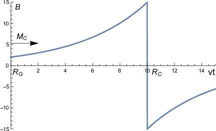
This type of models have been studied in the literature Jaffe:2019iuk but we simplify them further for our calculation. Let us assume that a monopolium cloud approaches the galaxy from the right and that the monopolium cloud is small enough compared with the size of the galaxy () that we can treat it as a point like object with mass . Thus we reduce the effective B field for the calculation to the one shown in Fig. 5.

We can formulate mathematically the magnetic field by
where the largest possible field found in galaxies, , and . We have chosen to plot the figure. Let the monopolium cloud move from the right towards the center with a velocity . The moving cloud feels a time dependent magnetic field , where is the point where we start measuring the time as can be seen in Fig. 6. The most interesting region is close to as we shall see.
The power emitted by a non harmonic force is Mirmoosa:2020pft
| (25) |
where , where recall that is the magnetic polarizability of monopolium, Eq.(22). The power can be written as
| (26) |
where , , and
being .
The emission of power taking into account the magnetic field direction is shown in Fig.7a which is the emitted wave signal. The total energy emitted in the process at the point is
| (28) |
In Fig. 7b we show the energy emitted as the cloud penetrates the galaxy noticing that most of the emission occurs precisely where the power wave is formed around and approximately during the interval .
If we integrate over the whole interval from to the origin we get
| (29) |
where
| (30) |
Note that is a numerical integral which dependes on the shape of the magnetic field and the structure of the galaxy as determined by the galaxy parameters but does not depend on the velocity. The only velocity dependence is in the factor in front of Eq.(29). is the less known parameter but it is smaller than the rest of size parameters. We use for the other size parameters realistic values as shown in the figures , which is the value of the highest possible galactic magnetic fields observed in nature, , , and for . This small value of makes the transition from one field direction to the other very abrupt.


Studying the dependence of the Integral on for small values of we find that it goes to a good approximation like a constant times as shown in Fig 8, i.e. . For the chosen values of the parameters the constant factor is approximately .
The emitted energy when the monopolium cloud passes across ,
| (31) |
where is the monopolium density which we parametrize by a temperature and its determined by the relation
| (32) |
where is the monopolium density today as shown in Eq.(11), and is the volume of the monopolium cloud. Assuming a spherical cloud we get for the energy emitted when the cloud passes across the region
| (33) |
where we have used the following units: is in fm3, in GeV/fm, in fm-3 which lead to an energy in GeV. The duration in passing the region is governed by the cloud diameter, . Using a favorable case where G, , , c, the emitted power is extremely small GeV/s Joule/s at emission. The smallness is associated with the smallness of the polarizability and also the small magnitude of the galactic fields. Thus monopolium matter associated with Kaluza-Klein monopoles is really dark and the fact that it is stable makes it very improbable to detect via its decay.

VI Concluding remarks
The existence of monopoles is a characteristic signature of Kaluza-Klein multidimensional theories Gross:1983hb; Sorkin:1983ns based on fundamental developments in lower dimensional theories Newman:1963yy; Hawking:1976jb; Gibbons:1979xm. The topology of these theories is extremely interesting, in particular the leitmotiv of my presentation is inspired by the existence of the dipole solution Gross:1983hb; Kerr:1963ud; Gibbons:1976ue, which has been associated to a monopole-anti-monopole bound state. In KK theories this state is classically stable since it does not have the quantum numbers of the vacuum and therefore is long lived. This state has been named monopolium. Its lowest energy state, i.e. and , is electromagnetically inert in free space. We have studied its properties and therefore suggest to propose it as a dark matter constituent.
In order to get some consequences of this line of thought we have used the details of the GPS model which makes the presentation simpler by dealing with exact formulas. But the outcome would be the same accepting some very general features: the topology Newman:1963yy; Hawking:1976jb; Gibbons:1979xm; Kerr:1963ud; Gibbons:1976ue ; the production mechanism by the compactification transition Zeldovich:1978wj; Preskill:1979zi; Harvey:1984fe ; the naturalness of parameters in terms of and . The only formula used from GPS can simply substituted by , where and by dimensional arguments. The only difference with the present calculation would be numerical coefficients, which are almost irrelevant, since what matters here are exponents.
Due to its huge mass, , KK monopoles can only be produced in large quantities via a compactification phase transition in the early Universe Harvey:1984fe. Their long range magnetic force will bind the KK poles form monopolium since monopoles and anti-monopoles are produced in equal quantitites. We have shown that there is a good chance that monopolium survives in detectable amounts after a conventional inflationary period and that their photon emission arising by de-excitation from the initially highly excited state to the ground state will not affect the cosmic microwave background. We have analyzed the observability of monopolium by using its electromagnetic properties induced in the presence of astronomical magnetic fields. We have seen that its magnetic polarizability is extremely small and thus detection is impossible even if appearing in large monopolium clouds. At this point we cannot think of any more favorable scenario than this one. There are objects, like magnetars Kaspi:2017fwg, with much higher magnetic fields, but these fields are of very small extension, at the level of kms, thus would be extremely small, and the emitted power even smaller than the one we have calculated. The other scenario we would like to study in the future is what happens with a cloud on monopolium in the proximity of a supermassive black holes in the center of the galaxies Ghez:2008ms; Gillessen:2008qv, but at this point we do not see how this phenomenon would increase observability. Thus KK monopolium seems very difficult to detect and therefore an ideal candidate to be one of the constituents of dark matter. Probably monopolium clouds will be only detectable by gravitational waves arising from their interaction with black holes.
What really remains to investigate is the discovery of possible signals to detect KK monopoles or KK monopolium. In this work we have assumed their existence and have described some properties which lead to monopolium as being a primordial dark matter constituent. But a proof, even a good argument of its existence is lacking. Its huge mass makes production unfeasible in accelerators, the small magnitude of its electromagnetic effects and its small present day density make it difficult to detect by astronomical observatories. Thus, the aim next is to search for properties of KK monopoles or KK monopolium, which help in proposing experiments which might prove or disprove its existence.
Acknowledgement
Discussions with Gabriela Barenboim, Huner Fanchiotti, Armando Pérez, Sergio Palomares, Santiago Noguera, and Javier Vijande are acknowledged. I would like to thank Carlos García Canal and Marco Traini for a careful reading of the manuscript and valuable comments and suggestions, and Marco Traini also for sharing his profound knowledge on polarizable systems with me. Conversations with V. Vento-Bosch were inspiring to initiate this study. This work was supported in part by the MICINN and UE Feder under contract FPA2016-77177-C2-1-P.
References
- (1) N. Aghanim et al. [Planck], Astron. Astrophys. 641 (2020), A6 doi:10.1051/0004-6361/201833910 [arXiv:1807.06209 [astro-ph.CO]].
- (2) R. H. Wechsler and J. L. Tinker, Ann. Rev. Astron. Astrophys. 56 (2018), 435-487 doi:10.1146/annurev-astro-081817-051756 [arXiv:1804.03097 [astro-ph.GA]].
- (3) G. ’t Hooft, Nucl. Phys. B 79 (1974) 276.
- (4) A. M. Polyakov, JETP Lett. 20 (1974) 194 [Pisma Zh. Eksp. Teor. Fiz. 20 (1974) 430].
- (5) H. Georgi and S. L. Glashow, Phys. Rev. Lett. 28 (1972) 1494.
- (6) J. Preskill, Ann. Rev. Nucl. Part. Sci. 34 (1984) 461. doi:10.1146/annurev.ns.34.120184.002333
- (7) Y. .M. Shnir, “Magnetic monopoles,” Berlin, Germany: Springer (2005) 532 p
- (8) A. H. Guth, Phys. Rev. D 23 (1981) 347 [Adv. Ser. Astrophys. Cosmol. 3 (1987) 139]. doi:10.1103/PhysRevD.23.347
- (9) A. D. Linde, Phys. Lett. 108B (1982) 389 [Adv. Ser. Astrophys. Cosmol. 3 (1987) 149]. doi:10.1016/0370-2693(82)91219-9
- (10) P. A. M. Dirac, Phys. Rev. 74 (1948), 817-830 doi:10.1103/PhysRev.74.817
- (11) T. Kaluza, Sitzungsber. Preuss. Akad. Wiss. Berlin (Math. Phys. ) 1921 (1921) 966 [Int. J. Mod. Phys. D 27 (2018) no.14, 1870001] doi:10.1142/S0218271818700017 [arXiv:1803.08616 [physics.hist-ph]].
- (12) O. Klein, Z. Phys. 37 (1926) 895 [Surveys High Energ. Phys. 5 (1986) 241]. doi:10.1007/BF01397481
- (13) D. J. Gross and M. J. Perry, Nucl. Phys. B 226 (1983) 29. doi:10.1016/0550-3213(83)90462-5
- (14) R. d. Sorkin, Phys. Rev. Lett. 51 (1983) 87. doi:10.1103/PhysRevLett.51.87
- (15) E. Newman, L. Tamburino and T. Unti, J. Math. Phys. 4 (1963) 915. doi:10.1063/1.1704018
- (16) S. W. Hawking, Phys. Lett. A 60 (1977) 81. doi:10.1016/0375-9601(77)90386-3
- (17) G. W. Gibbons and S. W. Hawking, Commun. Math. Phys. 66 (1979) 291. doi:10.1007/BF01197189
- (18) C. T. Hill, Nucl. Phys. B 224 (1983), 469-490 doi:10.1016/0550-3213(83)90386-3
- (19) V. Vento, Int. J. Mod. Phys. A 23 (2008), 4023-4037 doi:10.1142/S0217751X08041669 [arXiv:0709.0470 [astro-ph]].
- (20) L. N. Epele, H. Fanchiotti, C. A. Garcia Canal and V. Vento, Eur. Phys. J. C 56 (2008), 87-95 doi:10.1140/epjc/s10052-008-0628-0 [arXiv:hep-ph/0701133 [hep-ph]].
- (21) R. P. Kerr, Phys. Rev. Lett. 11 (1963), 237-238 doi:10.1103/PhysRevLett.11.237
- (22) G. W. Gibbons and S. W. Hawking, Phys. Rev. D 15 (1977), 2752-2756 doi:10.1103/PhysRevD.15.2752
- (23) J. M. Overduin and P. S. Wesson, Phys. Rept. 283 (1997), 303-380 doi:10.1016/S0370-1573(96)00046-4 [arXiv:gr-qc/9805018 [gr-qc]].
- (24) I. Zahed and G. E. Brown, Phys. Rept. 142 (1986), 1-102 doi:10.1016/0370-1573(86)90142-0
- (25) Z. F. Ezawa and I. G. Koh, Phys. Lett. 140B (1984) 205. doi:10.1016/0370-2693(84)90921-3
- (26) F. A. Bais and P. Batenburg, Nucl. Phys. B 253 (1985) 162. doi:10.1016/0550-3213(85)90524-3
- (27) S. C. Lee, Phys. Lett. 149B (1984) 100. doi:10.1016/0370-2693(84)91561-2
- (28) J. J. Xu and X. Li, Phys. Lett. B 208 (1988) 391. doi:10.1016/0370-2693(88)90635-1
- (29) R. B. Mann and C. Stelea, Nucl. Phys. B 729 (2005) 95 doi:10.1016/j.nuclphysb.2005.09.019 [hep-th/0505114].
- (30) I. I. Cotaescu, Nucl. Phys. B 719 (2005) 140 doi:10.1016/j.nuclphysb.2005.04.033 [hep-th/0501201].
- (31) T. Appelquist and A. Chodos, Phys. Rev. Lett. 50 (1983), 141 doi:10.1103/PhysRevLett.50.141
- (32) Y. B. Zeldovich and M. Y. Khlopov, Phys. Lett. B 79 (1978), 239-241 doi:10.1016/0370-2693(78)90232-0
- (33) J. Preskill, Phys. Rev. Lett. 43 (1979), 1365 doi:10.1103/PhysRevLett.43.1365
- (34) J. A. Harvey, E. W. Kolb and M. J. Perry, Phys. Lett. B 149 (1984), 465-469 doi:10.1016/0370-2693(84)90367-8
- (35) J. D. Jackson, Classical Electrodynamics, 3rd Edition 1998, John Willey and Sons, NY (USA).
- (36) T. R. Jaffe, Galaxies 7 (2019) no.2, 52 doi:10.3390/galaxies7020052 [arXiv:1904.12689 [astro-ph.GA]].
- (37) M. S. Mirmoosa, G. A. Ptitcyn, R Fleury and S.A. Tretyakov, Phys. Rev. A.102 no.1 013503
- (38) V. Vento and M. Traini, Eur. Phys. J. C 80 (2020) no.1, 62 doi:10.1140/epjc/s10052-020-7618-2 [arXiv:1909.03952 [hep-ph]].
- (39) V. M. Kaspi and A. Beloborodov, Ann. Rev. Astron. Astrophys. 55 (2017), 261-301 doi:10.1146/annurev-astro-081915-023329 [arXiv:1703.00068 [astro-ph.HE]].
- (40) A. M. Ghez, S. Salim, N. N. Weinberg, J. R. Lu, T. Do, J. K. Dunn, K. Matthews, M. Morris, S. Yelda and E. E. Becklin, et al. Astrophys. J. 689 (2008), 1044-1062 doi:10.1086/592738 [arXiv:0808.2870 [astro-ph]].
- (41) S. Gillessen, F. Eisenhauer, S. Trippe, T. Alexander, R. Genzel, F. Martins and T. Ott, Astrophys. J. 692 (2009), 1075-1109 doi:10.1088/0004-637X/692/2/1075 [arXiv:0810.4674 [astro-ph]].