跳到论文正文
W Papers独立论文阅读器 arXiv:2011.10271 论文正文 计算阅读时间 · 0%
引用这篇论文根据当前论文元数据生成,正式投稿前建议核对。


License: CC Zero
arXiv:2011.10271v1 [hep-ph] 20 Nov 2020

Prediction of neutron electromagnetic form factors behaviors just by the proton electromagnetic form factors data

Anna Z. Dubničková Address: Department of Theoretical Physics, Comenius University, Bratislava, Slovak Republic    Stanislav Dubnička Address: Institute of Physics, Slovak Academy of Sciences, Bratislava, Slovak Republic
August 11, 2026
Abstract

It is demonstrated how the neutron electromagnetic form factors behaviors in the whole region of their definition can be predicted theoretically just by using the proton form factors data to be described by the advanced proton electromagnetic structure Unitary and Analytic model.

Keywords: 
neutrons, protons, vector mesons, electromagnetic form factors, analyticity

I Introduction

Dominant building particles of the whole universe are protons pp and electrons ee. While the electron is always stable and a point-like particle up to now, the proton, though also to be stable, is compound of three quarks and as a result in interaction with electrons it appears as an extended object in the space. The latter property of the proton is called the proton electromagnetic (EM) structure, for the first time revealed in the middle of the last century, before the quark model of strongly interacting particles, hadrons, has been established. Later on this non-point-like nature of the proton has been generalized also to all other hadrons.

The EM structure of any hadron is completely described by scalar functions to be called EM form factors (FFs) of one variable, in the spacelike region it is the momentum transfer squared t=−Q2t=-Q^{2} and in timelike region it is the total c.m. energy squared s=w2s=w^{2}.

The number of EM FFs depends on the spin of the hadron under consideration. The EM structure of a hadron with spin 0 is completely described by one EM FF, the EM structure of a hadron with spin 1/2 is completely described by two EM FFs, the EM structure of a hadron with spin 1 is completely described by three EM FFs. In the case of the EM structure of hadrons with spin higher than one a situation is even more complicated and generally it is not solved satisfactorily up to now.

Further our interest will be concentrated to the 1/2+1/2^{+} octet baryons consisting of the following particles: p,n,Λ0,Σ+,Σ0,Σ−,Ξ0p,n,\Lambda^{0},\Sigma^{+},\Sigma^{0},\Sigma^{-},\Xi^{0} and Ξ−\Xi^{-}.

To know their EM structure means to have adequate multitude of as precise as possible experimental information on their EM FFs in the whole region of their definition and to dispose with reliable theoretical models to be able predict behaviors of these EM FFs consistently with data.

However, from all members of the 1/2+1/2^{+} octet baryons the most reliable and dense experimental data exist on the proton EM structure just due to its stability. They have been obtained by the processes like e−​p→e−​pe^{-}p\to e^{-}p, e+​p→e+​pe^{+}p\to e^{+}p, e+​e−→p​p¯e^{+}e^{-}\to p\bar{p}, p​p¯→e+​e−p\bar{p}\to e^{+}e^{-} and polarizations there. And thanks to a progress with more accomplished technologies one can expect even improved situation with these data in near future. Moreover the advanced proton EM structure U​n​i​t​a​r​y&A​n​a​l​y​t​i​cUnitary\&Analytic model ABDD has been constructed recently, which reproduces all existing data quite well.

The next member of the 1/2+1/2^{+} octet baryons is the neutron nn, for which there are no very precise and reliable experimental data just due to its instability. One is unable to prepare neither neutron targets nor antineutron beams for realization of similar experiments as they have been carried out with protons. In obtaining of the neutron EM FFs data a lot of model assumptions have been utilized and therefore finally the neutron data are not very reliable.

Heaving in mind the latter, in this paper we would like to demonstrate how the neutron EM FFs behaviors are predicted theoretically in the whole region of their definition by using the reliable proton EM FFs data, for a description of which the advanced proton EM structure U​n​i​t​a​r​y&A​n​a​l​y​t​i​cUnitary\&Analytic model ABDD is applied.

In the next papers a similar approach is planned to be realized also for other members of the 1/2+1/2^{+} octet baryons, so-called hyperons, starting with Λ0\Lambda^{0} and ending with Ξ\Xi hyperons, however for numerical estimation of free physically interpretable parameters of their U​n​i​t​a​r​y&A​n​a​l​y​t​i​cUnitary\&Analytic models a completely different and more laborious approach is developed.

II Proton electromagnetic structure model

The EM structure of the proton is completely described theoretically by two independent functions, the proton Dirac F1p​(t)F^{p}_{1}(t) and Pauli F2p​(t)F^{p}_{2}(t) FFs, which naturally appear in a decomposition of the proton matrix element of the EM current JμE​M​(0)J^{EM}_{\mu}(0) in the form of coefficients of two linearly independent covariants constructed from the four momenta p,p′p,p^{\prime}, γ\gamma-matrices and Dirac bi-spinors

<p|JμE​M​(0)|p>=e​u¯​(p′)​{γμ​F1p​(t)+i2​mp​σμ​ν​(p′−p)μ​F2p​(t)}​u​(p),\displaystyle<p|J^{EM}_{\mu}(0)|p>=e\bar{u}(p^{\prime})\{\gamma_{\mu}F^{p}_{1}(t)+\frac{i}{2m_{p}}\sigma_{\mu\nu}(p^{\prime}-p)_{\mu}F^{p}_{2}(t)\}u(p), (1)

with mpm_{p} to be the proton mass.

Description of the proton is even improved if the following mixed transformation properties of the EM current JμE​M​(0)J^{EM}_{\mu}(0) under the rotation in the isospin space are utilized. One its part transforms like isoscalar and another like the third component of isovector. These transformation properties lead to a splitting of the proton Dirac and Pauli EM FFs to flavour-independent isoscalar F1​sN​(t),F2​sN​(t)F^{N}_{1s}(t),F^{N}_{2s}(t) and isovector F1​vN​(t),F2​vN​(t)F^{N}_{1v}(t),F^{N}_{2v}(t) parts as follows

F1p​(t)=[F1​sN​(t)+F1​vN​(t)]\displaystyle F^{p}_{1}(t)=[F^{N}_{1s}(t)+F^{N}_{1v}(t)]
F2p​(t)=[F2​sN​(t)+F2​vN​(t)]\displaystyle F^{p}_{2}(t)=[F^{N}_{2s}(t)+F^{N}_{2v}(t)] (2)

whereby the sign between them is specified by the sign of the third component of the proton isospin to be +1/2+1/2.

The FFs F1​sN​(t),F1​vN​(t),F2​sN​(t),F2​vN​(t)F^{N}_{1s}(t),F^{N}_{1v}(t),F^{N}_{2s}(t),F^{N}_{2v}(t) are analytic in the whole complex t-plane besides the cuts on the positive real axis starting for isovector FFs at the two-pion threshold and for isoscalar FFs at three-pion threshold.

In the paper ABDD the advanced 9 vector-meson resonance
ρ⁡(770),ω⁡(782),ϕ⁡(1020);ρ′​(1450),ω′​(1420),ϕ′​(1680);ρ′′​(1700),ω′′​(1650),ϕ′′​(2170);\rho(770),\omega(782),\phi(1020);\rho^{\prime}(1450),\omega^{\prime}(1420),\phi^{\prime}(1680);\rho^{\prime\prime}(1700),\omega^{\prime\prime}(1650),\phi^{\prime\prime}(2170); PDG
Unitary and Analytic (U&A)(U\&A) model for proton isoscalar and isovector Dirac and Pauli FFs has been constructed

F1​sN[V(t)]=(1−V21−VN2)4{12Hω′′(V)Hϕ′′(V)\displaystyle F^{N}_{1s}[V(t)]=\Bigg(\frac{1-V^{2}}{1-V^{2}_{N}}\Bigg)^{4}\Bigg\{\frac{1}{2}H_{\omega^{\prime\prime}}(V)H_{\phi^{\prime\prime}}(V)
+[Hϕ′′(V)Hω′(V)(Cϕ′′1​s−Cω′1​s)(Cϕ′′1​s−Cω′′1​s)+Hω′′(V)Hω′(V)(Cω′′1​s−Cω′1​s)(Cω′′1​s−Cϕ′′1​s)\displaystyle+\Bigg[H_{\phi^{\prime\prime}}(V)H_{\omega^{\prime}}(V)\frac{(C^{1s}_{\phi^{\prime\prime}}-C^{1s}_{\omega^{\prime}})}{(C^{1s}_{\phi^{\prime\prime}}-C^{1s}_{\omega^{\prime\prime}})}+H_{\omega^{\prime\prime}}(V)H_{\omega^{\prime}}(V)\frac{(C^{1s}_{\omega^{\prime\prime}}-C^{1s}_{\omega^{\prime}})}{(C^{1s}_{\omega^{\prime\prime}}-C^{1s}_{\phi^{\prime\prime}})}
−Hω′′(V)Hϕ′′(V)](fω′​N​N(1)/fω′)\displaystyle-H_{\omega^{\prime\prime}}(V)H_{\phi^{\prime\prime}}(V)\Bigg](f^{(1)}_{\omega^{\prime}NN}/f_{\omega^{\prime}})
+[Hϕ′′(V)Hϕ′(V)(Cϕ′′1​s−Cϕ′1​s)(Cϕ′′1​s−Cω′′1​s)+Hω′′(V)Hϕ′(V)(Cω′′1​s−Cϕ′1​s)(Cω′′1​s−Cϕ′′1​s)\displaystyle+\Bigg[H_{\phi^{\prime\prime}}(V)H_{\phi^{\prime}}(V)\frac{(C^{1s}_{\phi^{\prime\prime}}-C^{1s}_{\phi^{\prime}})}{(C^{1s}_{\phi^{\prime\prime}}-C^{1s}_{\omega^{\prime\prime}})}+H_{\omega^{\prime\prime}}(V)H_{\phi^{\prime}}(V)\frac{(C^{1s}_{\omega^{\prime\prime}}-C^{1s}_{\phi^{\prime}})}{(C^{1s}_{\omega^{\prime\prime}}-C^{1s}_{\phi^{\prime\prime}})}
−Hω′′(V)Hϕ′′(V)](fϕ′​N​N(1)/fϕ′)\displaystyle-H_{\omega^{\prime\prime}}(V)H_{\phi^{\prime\prime}}(V)\Bigg](f^{(1)}_{\phi^{\prime}NN}/f_{\phi^{\prime}}) (3)
+[Hϕ′′(V)Lω(V)(Cϕ′′1​s−Cω1​s)(Cϕ′′1​s−Cω′′1​s)+Hω′′(V)Lω(V)(Cω′′1​s−Cω1​s)(Cω′′1​s−Cϕ′′1​s)\displaystyle+\Bigg[H_{\phi^{\prime\prime}}(V)L_{\omega}(V)\frac{(C^{1s}_{\phi^{\prime\prime}}-C^{1s}_{\omega})}{(C^{1s}_{\phi^{\prime\prime}}-C^{1s}_{\omega^{\prime\prime}})}+H_{\omega^{\prime\prime}}(V)L_{\omega}(V)\frac{(C^{1s}_{\omega^{\prime\prime}}-C^{1s}_{\omega})}{(C^{1s}_{\omega^{\prime\prime}}-C^{1s}_{\phi^{\prime\prime}})}
−Hω′′(V)Hϕ′′(V)](fω​N​N(1)/fω)\displaystyle-H_{\omega^{\prime\prime}}(V)H_{\phi^{\prime\prime}}(V)\Bigg](f^{(1)}_{\omega NN}/f_{\omega})
+[Hϕ′′(V)Lϕ(V)(Cϕ′′1​s−Cϕ1​s)(Cϕ′′1​s−Cω′′1​s)+Hω′′(V)Lϕ(V)(Cω′′1​s−Cϕ1​s)(Cω′′1​s−Cϕ′′1​s)\displaystyle+\Bigg[H_{\phi^{\prime\prime}}(V)L_{\phi}(V)\frac{(C^{1s}_{\phi^{\prime\prime}}-C^{1s}_{\phi})}{(C^{1s}_{\phi^{\prime\prime}}-C^{1s}_{\omega^{\prime\prime}})}+H_{\omega^{\prime\prime}}(V)L_{\phi}(V)\frac{(C^{1s}_{\omega^{\prime\prime}}-C^{1s}_{\phi})}{(C^{1s}_{\omega^{\prime\prime}}-C^{1s}_{\phi^{\prime\prime}})}
−Hω′′(V)Hϕ′′(V)](fϕ​N​N(1)/fϕ)}\displaystyle-H_{\omega^{\prime\prime}}(V)H_{\phi^{\prime\prime}}(V)\Bigg](f^{(1)}_{\phi NN}/f_{\phi})\Bigg\}

with 5 free parameters (fω′​N​N(1)/fω′),(fϕ′​N​N(1)/fϕ′),(fω​N​N(1)/fω),(fϕ​N​N(1)/fϕ),ti​n1​s(f^{(1)}_{\omega^{\prime}NN}/f_{\omega^{\prime}}),(f^{(1)}_{\phi^{\prime}NN}/f_{\phi^{\prime}}),(f^{(1)}_{\omega NN}/f_{\omega}),(f^{(1)}_{\phi NN}/f_{\phi}),t^{1s}_{in}

F1​vN[W(t)]=(1−W21−WN2)4{12Lρ(W)Lρ′(W)\displaystyle F^{N}_{1v}[W(t)]=\Bigg(\frac{1-W^{2}}{1-W^{2}_{N}}\Bigg)^{4}\Bigg\{\frac{1}{2}L_{\rho}(W)L_{\rho^{\prime}}(W)
+[Lρ′(W)Lρ′′(W)(Cρ′1​v−Cρ′′1​v)(Cρ′1​v−Cρ1​v)+Lρ(W)Lρ′′(W)(Cρ1​v−Cρ′′1​v)(Cρ1​v−Cρ′1​v)\displaystyle+\Bigg[L_{\rho^{\prime}}(W)L_{\rho^{\prime\prime}}(W)\frac{(C^{1v}_{\rho^{\prime}}-C^{1v}_{\rho^{\prime\prime}})}{(C^{1v}_{\rho^{\prime}}-C^{1v}_{\rho})}+L_{\rho}(W)L_{\rho^{\prime\prime}}(W)\frac{(C^{1v}_{\rho}-C^{1v}_{\rho^{\prime\prime}})}{(C^{1v}_{\rho}-C^{1v}_{\rho^{\prime}})} (4)
−Lρ(W)Lρ′(W)](fρ​N​N(1)/fρ)}\displaystyle-L_{\rho}(W)L_{\rho^{\prime}}(W)\Bigg](f^{(1)}_{\rho NN}/f_{\rho})\Bigg\}

with 2 free parameters (fρ​N​N(1)/fρ)(f^{(1)}_{\rho NN}/f_{\rho}) and ti​n1​vt^{1v}_{in},

F2​sN[U(t)]=(1−U21−UN2)6{12(μp+μn−1)Hω′′(U)Hϕ′′(U)Hω′(U)\displaystyle F^{N}_{2s}[U(t)]=\Bigg(\frac{1-U^{2}}{1-U^{2}_{N}}\Bigg)^{6}\Bigg\{\frac{1}{2}(\mu_{p}+\mu_{n}-1)H_{\omega^{\prime\prime}}(U)H_{\phi^{\prime\prime}}(U)H_{\omega^{\prime}}(U)
+[Hϕ′′(U)Hω′(U)Hϕ′(U)(Cϕ′′2​s−Cϕ′2​s)​(Cω′2​s−Cϕ′2​s)(Cϕ′′2​s−Cω′′2​s)​(Cω′2​s−Cω′′2​s)\displaystyle+\Bigg[H_{\phi^{\prime\prime}}(U)H_{\omega^{\prime}}(U)H_{\phi^{\prime}}(U)\frac{(C^{2s}_{\phi^{\prime\prime}}-C^{2s}_{\phi^{\prime}})(C^{2s}_{\omega^{\prime}}-C^{2s}_{\phi^{\prime}})}{(C^{2s}_{\phi^{\prime\prime}}-C^{2s}_{\omega^{\prime\prime}})(C^{2s}_{\omega^{\prime}}-C^{2s}_{\omega^{\prime\prime}})}
+Hω′′​(U)​Hω′​(U)​Hϕ′​(U)​(Cω′′2​s−Cϕ′2​s)​(Cω′2​s−Cϕ′2​s)(Cω′′2​s−Cϕ′′2​s)​(Cω′2​s−Cϕ′′2​s)\displaystyle+H_{\omega^{\prime\prime}}(U)H_{\omega^{\prime}}(U)H_{\phi^{\prime}}(U)\frac{(C^{2s}_{\omega^{\prime\prime}}-C^{2s}_{\phi^{\prime}})(C^{2s}_{\omega^{\prime}}-C^{2s}_{\phi^{\prime}})}{(C^{2s}_{\omega^{\prime\prime}}-C^{2s}_{\phi^{\prime\prime}})(C^{2s}_{\omega^{\prime}}-C^{2s}_{\phi^{\prime\prime}})}
+Hω′′​(U)​Hϕ′′​(U)​Hϕ′​(U)​(Cω′′2​s−Cϕ′2​s)​(Cϕ′′2​s−Cϕ′2​s)(Cω′′2​s−Cω′2​s)​(Cϕ′′2​s−Cω′2​s)\displaystyle+H_{\omega^{\prime\prime}}(U)H_{\phi^{\prime\prime}}(U)H_{\phi^{\prime}}(U)\frac{(C^{2s}_{\omega^{\prime\prime}}-C^{2s}_{\phi^{\prime}})(C^{2s}_{\phi^{\prime\prime}}-C^{2s}_{\phi^{\prime}})}{(C^{2s}_{\omega^{\prime\prime}}-C^{2s}_{\omega^{\prime}})(C^{2s}_{\phi^{\prime\prime}}-C^{2s}_{\omega^{\prime}})}
−Hω′′(U)Hϕ′′(U)Hω′(U)](fϕ′​N​N(2)/fϕ′)\displaystyle-H_{\omega^{\prime\prime}}(U)H_{\phi^{\prime\prime}}(U)H_{\omega^{\prime}}(U)\Bigg](f^{(2)}_{\phi^{\prime}NN}/f_{\phi^{\prime}})
+[Hϕ′′(U)Hω′(U)Lω(U)(Cϕ′′2​s−Cω2​s)​(Cω′2​s−Cω2​s)(Cϕ′′2​s−Cω′′2​s)​(Cω′2​s−Cω′′2​s)\displaystyle+\Bigg[H_{\phi^{\prime\prime}}(U)H_{\omega^{\prime}}(U)L_{\omega}(U)\frac{(C^{2s}_{\phi^{\prime\prime}}-C^{2s}_{\omega})(C^{2s}_{\omega^{\prime}}-C^{2s}_{\omega})}{(C^{2s}_{\phi^{\prime\prime}}-C^{2s}_{\omega^{\prime\prime}})(C^{2s}_{\omega^{\prime}}-C^{2s}_{\omega^{\prime\prime}})}
+Hω′′​(U)​Hω′​(U)​Lω​(U)​(Cω′′2​s−Cω2​s)​(Cω′2​s−Cω2​s)(Cω′′2​s−Cϕ′′2​s)​(Cω′2​s−Cϕ′′2​s)+\displaystyle+H_{\omega^{\prime\prime}}(U)H_{\omega^{\prime}}(U)L_{\omega}(U)\frac{(C^{2s}_{\omega^{\prime\prime}}-C^{2s}_{\omega})(C^{2s}_{\omega^{\prime}}-C^{2s}_{\omega})}{(C^{2s}_{\omega^{\prime\prime}}-C^{2s}_{\phi^{\prime\prime}})(C^{2s}_{\omega^{\prime}}-C^{2s}_{\phi^{\prime\prime}})}+
+Hω′′​(U)​Hϕ′′​(U)​Lω​(U)​(Cω′′2​s−Cω2​s)​(Cϕ′2​s−Cω2​s)(Cω′′2​s−Cω′2​s)​(Cϕ′′2​s−Cω′2​s)\displaystyle+H_{\omega^{\prime\prime}}(U)H_{\phi^{\prime\prime}}(U)L_{\omega}(U)\frac{(C^{2s}_{\omega^{\prime\prime}}-C^{2s}_{\omega})(C^{2s}_{\phi^{\prime}}-C^{2s}_{\omega})}{(C^{2s}_{\omega^{\prime\prime}}-C^{2s}_{\omega^{\prime}})(C^{2s}_{\phi^{\prime\prime}}-C^{2s}_{\omega^{\prime}})} (5)
−Hω′′(U)Hϕ′′(U)Hω′(U)](fω​N​N(2)/fω)\displaystyle-H_{\omega^{\prime\prime}}(U)H_{\phi^{\prime\prime}}(U)H_{\omega^{\prime}}(U)\Bigg](f^{(2)}_{\omega NN}/f_{\omega})
+[Hϕ′′(U)Hω′(U)Lϕ(U)(Cϕ′′2​s−Cϕ2​s)​(Cω′2​s−Cϕ2​s)(Cϕ′′2​s−Cω′′2​s)​(Cω′2​s−Cω′′2​s)\displaystyle+\Bigg[H_{\phi^{\prime\prime}}(U)H_{\omega^{\prime}}(U)L_{\phi}(U)\frac{(C^{2s}_{\phi^{\prime\prime}}-C^{2s}_{\phi})(C^{2s}_{\omega^{\prime}}-C^{2s}_{\phi})}{(C^{2s}_{\phi^{\prime\prime}}-C^{2s}_{\omega^{\prime\prime}})(C^{2s}_{\omega^{\prime}}-C^{2s}_{\omega^{\prime\prime}})}
+Hω′′​(U)​Hω′​(U)​Lϕ​(U)​(Cω′′2​s−Cϕ2​s)​(Cω′2​s−Cϕ2​s)(Cω′′2​s−Cϕ′′2​s)​(Cω′2​s−Cϕ′′2​s)\displaystyle+H_{\omega^{\prime\prime}}(U)H_{\omega^{\prime}}(U)L_{\phi}(U)\frac{(C^{2s}_{\omega^{\prime\prime}}-C^{2s}_{\phi})(C^{2s}_{\omega^{\prime}}-C^{2s}_{\phi})}{(C^{2s}_{\omega^{\prime\prime}}-C^{2s}_{\phi^{\prime\prime}})(C^{2s}_{\omega^{\prime}}-C^{2s}_{\phi^{\prime\prime}})}
+Hω′′​(U)​Hϕ′′​(U)​Lϕ​(U)​(Cω′′2​s−Cϕ2​s)​(Cϕ′′2​s−Cϕ2​s)(Cω′′2​s−Cω′2​s)​(Cϕ′′2​s−Cω′2​s)\displaystyle+H_{\omega^{\prime\prime}}(U)H_{\phi^{\prime\prime}}(U)L_{\phi}(U)\frac{(C^{2s}_{\omega^{\prime\prime}}-C^{2s}_{\phi})(C^{2s}_{\phi^{\prime\prime}}-C^{2s}_{\phi})}{(C^{2s}_{\omega^{\prime\prime}}-C^{2s}_{\omega^{\prime}})(C^{2s}_{\phi^{\prime\prime}}-C^{2s}_{\omega^{\prime}})}
−Hω′′(U)Hϕ′′(U)Hω′(U)](fϕ​N​N(2)/fϕ)}\displaystyle-H_{\omega^{\prime\prime}}(U)H_{\phi^{\prime\prime}}(U)H_{\omega^{\prime}}(U)\Bigg](f^{(2)}_{\phi NN}/f_{\phi})\Bigg\}

with 4 free parameters (fϕ′​N​N(2)/fϕ′)(f^{(2)}_{\phi^{\prime}NN}/f_{\phi^{\prime}}), (fω​N​N(2)/fω)(f^{(2)}_{\omega NN}/f_{\omega}), (fϕ​N​N(2)/fϕ),ti​n2​s(f^{(2)}_{\phi NN}/f_{\phi}),t^{2s}_{in}, and

F2​vN​[X⁡(t)]=(1−X21−XN2)6​{12​(μp−μn−1)​Lρ​(X)​Lρ′​(X)​Hρ′′​(X)}\displaystyle F^{N}_{2v}[X(t)]=\Bigg(\frac{1-X^{2}}{1-X^{2}_{N}}\Bigg)^{6}\Bigg\{\frac{1}{2}(\mu_{p}-\mu_{n}-1)L_{\rho}(X)L_{\rho^{\prime}}(X)H_{\rho^{\prime\prime}}(X)\Bigg\} (6)

dependent on only 1 free parameter ti​n2​vt^{2v}_{in} with

Lr​(V)=(VN−Vr)​(VN−Vr∗)​(VN−1/Vr)​(VN−1/Vr∗)(V−Vr)​(V−Vr∗)​(V−1/Vr)​(V−1/Vr∗),\displaystyle L_{r}(V)=\frac{(V_{N}-V_{r})(V_{N}-V^{*}_{r})(V_{N}-1/V_{r})(V_{N}-1/V^{*}_{r})}{(V-V_{r})(V-V^{*}_{r})(V-1/V_{r})(V-1/V^{*}_{r})}, (7)
C1​sr=(VN−Vr)​(VN−Vr∗)​(VN−1/Vr)​(VN−1/Vr∗)−(Vr−1/Vr)​(Vr−1/Vr∗),r=ω,ϕ\displaystyle C^{1s}_{r}=\frac{(V_{N}-V_{r})(V_{N}-V^{*}_{r})(V_{N}-1/V_{r})(V_{N}-1/V^{*}_{r})}{-(V_{r}-1/V_{r})(V_{r}-1/V^{*}_{r})},r=\omega,\phi
Hl​(V)=(VN−Vl)​(VN−Vl∗)​(VN+Vl)​(VN+Vl∗)(V−Vl)​(V−Vl∗)​(V+Vl)​(V+Vl∗),\displaystyle H_{l}(V)=\frac{(V_{N}-V_{l})(V_{N}-V^{*}_{l})(V_{N}+V_{l})(V_{N}+V^{*}_{l})}{(V-V_{l})(V-V^{*}_{l})(V+V_{l})(V+V^{*}_{l})}, (8)
C1​sl=(VN−Vl)​(VN−Vl∗)​(VN+Vl)​(VN+Vl∗)−(Vl−1/Vl)​(Vl−1/Vl∗),l=ω′′,ϕ′′,ω′,ϕ′\displaystyle C^{1s}_{l}=\frac{(V_{N}-V_{l})(V_{N}-V^{*}_{l})(V_{N}+V_{l})(V_{N}+V^{*}_{l})}{-(V_{l}-1/V_{l})(V_{l}-1/V^{*}_{l})},l=\omega^{\prime\prime},\phi^{\prime\prime},\omega^{\prime},\phi^{\prime}
Lk​(W)=(WN−Wk)​(WN−Wk∗)​(WN−1/Wk)​(WN−1/Wk∗)(W−Wk)​(W−Wk∗)​(W−1/Wk)​(W−1/Wk∗),\displaystyle L_{k}(W)=\frac{(W_{N}-W_{k})(W_{N}-W^{*}_{k})(W_{N}-1/W_{k})(W_{N}-1/W^{*}_{k})}{(W-W_{k})(W-W^{*}_{k})(W-1/W_{k})(W-1/W^{*}_{k})}, (9)
C1​vk=(WN−Wk)​(WN−Wk∗)​(WN−1/Wk)​(WN−1/Wk∗)−(Wk−1/Wk)​(Wk−1/Wk∗),k=ρ′′,ρ′,ρ\displaystyle C^{1v}_{k}=\frac{(W_{N}-W_{k})(W_{N}-W^{*}_{k})(W_{N}-1/W_{k})(W_{N}-1/W^{*}_{k})}{-(W_{k}-1/W_{k})(W_{k}-1/W^{*}_{k})},k=\rho^{\prime\prime},\rho^{\prime},\rho
Lr​(U)=(UN−Ur)​(UN−Ur∗)​(UN−1/Ur)​(UN−1/Ur∗)(U−Ur)​(U−Ur∗)​(U−1/Ur)​(U−1/Ur∗),\displaystyle L_{r}(U)=\frac{(U_{N}-U_{r})(U_{N}-U^{*}_{r})(U_{N}-1/U_{r})(U_{N}-1/U^{*}_{r})}{(U-U_{r})(U-U^{*}_{r})(U-1/U_{r})(U-1/U^{*}_{r})}, (10)
C2​sr=(UN−Ur)​(UN−Ur∗)​(UN−1/Ur)​(UN−1/Ur∗)−(Ur−1/Ur)​(Ur−1/Ur∗),r=ω,ϕ\displaystyle C^{2s}_{r}=\frac{(U_{N}-U_{r})(U_{N}-U^{*}_{r})(U_{N}-1/U_{r})(U_{N}-1/U^{*}_{r})}{-(U_{r}-1/U_{r})(U_{r}-1/U^{*}_{r})},r=\omega,\phi
Hl​(U)=(UN−Ul)​(UN−Ul∗)​(UN+Ul)​(UN+Ul∗)(U−Ul)​(U−Ul∗)​(U+Ul)​(U+Ul∗),\displaystyle H_{l}(U)=\frac{(U_{N}-U_{l})(U_{N}-U^{*}_{l})(U_{N}+U_{l})(U_{N}+U^{*}_{l})}{(U-U_{l})(U-U^{*}_{l})(U+U_{l})(U+U^{*}_{l})}, (11)
C2​sl=(UN−Ul)​(UN−Ul∗)​(UN+Ul)​(UN+Ul∗)−(Ul−1/Ul)​(Ul−1/Ul∗),l=ω′′,ϕ′′,ω′,ϕ′\displaystyle C^{2s}_{l}=\frac{(U_{N}-U_{l})(U_{N}-U^{*}_{l})(U_{N}+U_{l})(U_{N}+U^{*}_{l})}{-(U_{l}-1/U_{l})(U_{l}-1/U^{*}_{l})},l=\omega^{\prime\prime},\phi^{\prime\prime},\omega^{\prime},\phi^{\prime}
Lk​(X)=(XN−Xk)​(XN−Xk∗)​(XN−1/Xk)​(XN−1/Xk∗)(X−Xk)​(X−Xk∗)​(X−1/Xk)​(X−1/Xk∗),\displaystyle L_{k}(X)=\frac{(X_{N}-X_{k})(X_{N}-X^{*}_{k})(X_{N}-1/X_{k})(X_{N}-1/X^{*}_{k})}{(X-X_{k})(X-X^{*}_{k})(X-1/X_{k})(X-1/X^{*}_{k})}, (12)
C2​vk=(XN−Xk)​(XN−Xk∗)​(XN−1/Xk)​(XN−1/Xk∗)−(Xk−1/Xk)​(Xk−1/Xk∗),k=ρ′,ρ\displaystyle C^{2v}_{k}=\frac{(X_{N}-X_{k})(X_{N}-X^{*}_{k})(X_{N}-1/X_{k})(X_{N}-1/X^{*}_{k})}{-(X_{k}-1/X_{k})(X_{k}-1/X^{*}_{k})},k=\rho^{\prime},\rho
Hρ′′​(X)=(XN−Xρ′′)​(XN−Xρ′′∗)​(XN+Xρ′′)​(XN+Xρ′′∗)(X−Xρ′′)​(X−Xρ′′∗)​(X+Xρ′′)​(X+Xρ′′∗),\displaystyle H_{\rho^{\prime\prime}}(X)=\frac{(X_{N}-X_{\rho^{\prime\prime}})(X_{N}-X^{*}_{\rho^{\prime\prime}})(X_{N}+X_{\rho^{\prime\prime}})(X_{N}+X^{*}_{\rho^{\prime\prime}})}{(X-X_{\rho^{\prime\prime}})(X-X^{*}_{\rho^{\prime\prime}})(X+X_{\rho^{\prime\prime}})(X+X^{*}_{\rho^{\prime\prime}})}, (13)
Cρ′′2​v=(XN−Xρ′′)​(XN−Xρ′′∗)​(XN+Xρ′′)​(XN+Xρ′′∗)−(Xρ′′−1/Xρ′′)​(Xρ′′−1/Xρ′′∗).\displaystyle C^{2v}_{\rho^{\prime\prime}}=\frac{(X_{N}-X_{\rho^{\prime\prime}})(X_{N}-X^{*}_{\rho^{\prime\prime}})(X_{N}+X_{\rho^{\prime\prime}})(X_{N}+X^{*}_{\rho^{\prime\prime}})}{-(X_{\rho^{\prime\prime}}-1/X_{\rho^{\prime\prime}})(X_{\rho^{\prime\prime}}-1/X^{*}_{\rho^{\prime\prime}})}.

Whereas the Dirac F1p​(t)F^{p}_{1}(t) and Pauli F2p​(t)F^{p}_{2}(t) proton FFs, as it is seen from the previous, are very effective for theoretical considerations of the proton EM structure, an extraction of experimental information on it from measured cross sections and polarizations, by the proton electric GEp​(t)G^{p}_{E}(t) and proton magnetic GMp​(t)G^{p}_{M}(t) FFs is more comfortable. They appear e.g. in the total cross section of e+​e−→p​p¯e^{+}e^{-}\to p\bar{p} process BPZZ

σt​o​t​(e+​e−→p​p¯)=4​π​α2​C​βp​(t)3​t​[|GMp​(t)|2+2​mpt​|GEp​(s)|2]\displaystyle\sigma_{tot}(e^{+}e^{-}\to p\bar{p})=\frac{4\pi\alpha^{2}C\beta_{p}(t)}{3t}[|G^{p}_{M}(t)|^{2}+\frac{2m_{p}}{t}|G^{p}_{E}(s)|^{2}] (14)

with βp​(t)=1−4​mp2t\beta_{p}(t)=\sqrt{1-\frac{4m^{2}_{p}}{t}} and CC to be the Coulomb enhancement factor, without interference term, unlike the case if Dirac and Pauli FFs appear in the same total cross section.

The relations between both sets of FFs are

GEp​(t)=[F1​sN​(t)+F1​vN​(t)]+t4​mp2​[F2​sN​(t)+F2​vN​(t)]\displaystyle G^{p}_{E}(t)=[F^{N}_{1s}(t)+F^{N}_{1v}(t)]+\frac{t}{4m^{2}_{p}}[F^{N}_{2s}(t)+F^{N}_{2v}(t)] (15)
GMp​(t)=[F1​sN​(t)+F1​vN​(t)]+[F2​sN​(t)+F2​vN​(t)]\displaystyle G^{p}_{M}(t)=[F^{N}_{1s}(t)+F^{N}_{1v}(t)]+[F^{N}_{2s}(t)+F^{N}_{2v}(t)]

with normalizations

GEp​(0)=1;GMp​(0)=μp;\displaystyle G^{p}_{E}(0)=1;\quad G^{p}_{M}(0)=\mu_{p}; (16)

and

F1​sN​(0)=F1​vN​(0)=12;F2​sN​(0)=12​(μp+μn−1);F2​vN​(0)=12​(μp−μn−1),\displaystyle F^{N}_{1s}(0)=F^{N}_{1v}(0)=\frac{1}{2};\quad F^{N}_{2s}(0)=\frac{1}{2}(\mu_{p}+\mu_{n}-1);\quad F^{N}_{2v}(0)=\frac{1}{2}(\mu_{p}-\mu_{n}-1), (17)

where μp\mu_{p} and μn\mu_{n} are the magnetic moments of the proton and neutron, respectively.

The model is in fact a well-matched unification of pole contributions of unstable vector mesons with cut structure in the complex plane tt, whereby these cuts represent so-called continua contributions generated by exchange of more than one particle in the corresponding Feynman diagrams and they secure FFs imaginary parts to be different from zero just beyond the lowest possible thresholds on the positive real axis, as it is required by the FFs unitarity conditions.

There are approximately 460 more or less reliable experimental points on the proton EM FFs GEp​(t),GMp​(t)G^{p}_{E}(t),G^{p}_{M}(t) jones-Ab1 to be graphically presented in Figs. 1-2.

Refer to caption
Refer to caption
Figure 1: Experimental data on the ratios of the proton electric to magnetic FFs in space-like and time-like regions.

The results of their simultaneous analysis by the proton EM structure U&AU\&A model given by (II)-(6) and (15) with 12 free parameters with a clear physical meaning are given in TABLE.

Refer to caption
Refer to caption
Figure 2: Experimental data on the proton electric and magnetic FFs in space-like and time-like regions.

TABLE: Values of free parameters of the proton EM structure U&AU\&A model evaluated in the analysis of the proton EM FFs data.
χ2/n​d​f=1.74;\chi^{2}/ndf=1.74;  si​n1​s=(1.6750±0.0363)​G​e​V2;si​n1​v=(2.9683±0.0091)​G​e​V2;s^{1s}_{in}=(1.6750\pm 0.0363)GeV^{2};s^{1v}_{in}=(2.9683\pm 0.0091)GeV^{2};
si​n2​s=(1.8590±0.0023)​G​e​V2;si​n2​v=(2.4425±0.0208)​G​e​V2;s^{2s}_{in}=(1.8590\pm 0.0023)GeV^{2};s^{2v}_{in}=(2.4425\pm 0.0208)GeV^{2};
(fω′​N​N(1)/fω′)=−0.2937±0.0015;(fϕ′​N​N(1)/fϕ′)=−0.5298±0.0027;(fω​N​N(1)/fω)=0.6384±0.0025;(fϕ​N​N(1)/fϕ)=−0.0271±0.0005;(fϕ′​N​N(2)/fϕ′)=0.3075±0.0156;(fω​N​N(2)/fω)=0.1676±0.0377;(fϕ​N​N(2)/fϕ)=0.1226±0.0035;(fρ​N​N(1)/fρ)=−0.0802±0.0014;(f^{(1)}_{\omega^{\prime}NN}/f_{\omega^{\prime}})=-0.2937\pm 0.0015;(f^{(1)}_{\phi^{\prime}NN}/f_{\phi^{\prime}})=-0.5298\pm 0.0027;\\ (f^{(1)}_{\omega NN}/f_{\omega})=0.6384\pm 0.0025;(f^{(1)}_{\phi NN}/f_{\phi})=-0.0271\pm 0.0005;\\ (f^{(2)}_{\phi^{\prime}NN}/f_{\phi^{\prime}})=0.3075\pm 0.0156;(f^{(2)}_{\omega NN}/f_{\omega})=0.1676\pm 0.0377;\\ (f^{(2)}_{\phi NN}/f_{\phi})=0.1226\pm 0.0035;(f^{(1)}_{\rho NN}/f_{\rho})=-0.0802\pm 0.0014;

The corresponding behaviors of absolute values of the proton electric and magnetic FFs on the base of these results are given by full lines in Fig. 3, where also their comparison with exiting data is presented.

Refer to caption
Refer to caption
Figure 3: The proton EM structure U&AU\&A model given by (II)-(6) and (15) with parameters of TABLE reproduce existing data quite well.

III Theoretical predictions of neutron electromagnetic form factors behaviors

Similarly to the proton one can define the neutron Dirac F1n​(t)F^{n}_{1}(t) and Pauli F2n​(t)F^{n}_{2}(t) FFs by means of the neutron matrix element of the EM current JμE​M​(0)J^{EM}_{\mu}(0)

<n|JμE​M​(0)|n>=e​u¯​(p′)​{γμ​F1n​(t)+i2​mn​σμ​ν​(p′−p)μ​F2n​(t)}​u​(p),\displaystyle<n|J^{EM}_{\mu}(0)|n>=e\bar{u}(p^{\prime})\{\gamma_{\mu}F^{n}_{1}(t)+\frac{i}{2m_{n}}\sigma_{\mu\nu}(p^{\prime}-p)_{\mu}F^{n}_{2}(t)\}u(p), (18)

with mnm_{n} to be the neutron mass. Again mixed transformation properties of the EM current JμE​M​(0)J^{EM}_{\mu}(0) under the rotation in the isospin space is utilized, which leads to a splitting of the neutron Dirac F1n​(t)F^{n}_{1}(t) and Pauli F2n​(t)F^{n}_{2}(t) FFs to the same flavour-independent isoscalar F1​sN​(t),F2​sN​(t)F^{N}_{1s}(t),F^{N}_{2s}(t) and isovector F1​vN​(t),F2​vN​(t)F^{N}_{1v}(t),F^{N}_{2v}(t) parts like in the case of the proton as follows

F1n​(t)=[F1​sN​(t)−F1​vN​(t)]\displaystyle F^{n}_{1}(t)=[F^{N}_{1s}(t)-F^{N}_{1v}(t)]
F2n​(t)=[F2​sN​(t)−F2​vN​(t)]\displaystyle F^{n}_{2}(t)=[F^{N}_{2s}(t)-F^{N}_{2v}(t)] (19)

however, now with the minus sign between them as the sign of the third component of the neutron isospin is -1/2.

Refer to caption
Refer to caption
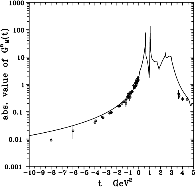
Figure 4: Predicted absolute value of the neutron electric and magnetic FFs behaviors without the use of any experimental point hanson-riordan seen in this figures.

Then the relations between neutron EM FFs and the flavour-independent neutron Dirac and Pauli FFs are

GEn​(t)=[F1​sN​(t)−F1​vN​(t)]+t4​mn2​[F2​sN​(t)−F2​vN​(t)]\displaystyle G^{n}_{E}(t)=[F^{N}_{1s}(t)-F^{N}_{1v}(t)]+\frac{t}{4m^{2}_{n}}[F^{N}_{2s}(t)-F^{N}_{2v}(t)] (20)
GMn​(t)=[F1​sN​(t)−F1​vN​(t)]+[F2​sN​(t)−F2​vN​(t)]\displaystyle G^{n}_{M}(t)=[F^{N}_{1s}(t)-F^{N}_{1v}(t)]+[F^{N}_{2s}(t)-F^{N}_{2v}(t)]

with normalizations

GEn​(0)=0;GMn​(0)=μn.\displaystyle G^{n}_{E}(0)=0;\quad G^{n}_{M}(0)=\mu_{n}. (21)

Since the FFs F1​sN​(t),F2​sN​(t)F^{N}_{1s}(t),F^{N}_{2s}(t) and F1​vN​(t),F2​vN​(t)F^{N}_{1v}(t),F^{N}_{2v}(t) are completely known by the expressions (II)-(6) with free parameters from TABLE to be evaluated in the analysis of only the proton EM FFs data, in combination with relations (20) they represent the advanced neutron electromagnetic structure U&AU\&A model, which enables to predict behaviors of the absolute values of the neutron electric GEn​(t)G^{n}_{E}(t) and magnetic GMn​(t)G^{n}_{M}(t) FFs theoretically, as they are presented by the full lines in Fig. 4, without the use of any experimental point hanson-riordan on the neutron EM FFs data also shown there for a comparison. The results are encouraging.

IV Conclusions

The absolute values of the neutron EM FFs, GEn​(t),GMn​(t)G^{n}_{E}(t),G^{n}_{M}(t), are predicted theoretically in the whole region of their definition without exploiting of any experimental point on them. This could be carried out by the fact that the proton EM structure U&AU\&A model given by (II)-(6) and (15) and the neutron EM structure U&AU\&A model given by (II)-(6) and (20) are compound of the same flavour-independent isoscalar F1​sN​(t),F2​sN​(t)F^{N}_{1s}(t),F^{N}_{2s}(t) and isovector F1​vN​(t),F2​vN​(t)F^{N}_{1v}(t),F^{N}_{2v}(t) parts of the corresponding Dirac and Pauli FFs, and it does not matter that in the case of the proton with "+" sign and in the case of the neutron with "-" sign, however, they depend on the same free parameters.

So, these parameters can be numerically evaluated either in the analysis of the neutron EM FFs data by means of the neutron EM structure U&AU\&A model and then one predicts absolute values of the proton EM FFs behaviors, or in the analysis of the proton EM FFs data by means of the proton EM structure U&AU\&A model and then one predicts absolute values of the neutron EM FFs behaviors. Naturally, as at present the proton EM FFs are more reliable and more precise, we have preferred the second case.

On the conclusion we would like to emphasize that if more precise and more reliable proton EM FFs data will appear in as wide region of their definition as possible, the more reliable predictions for the absolute values of the neutron EM FFs will be achieved by the approach discussed in this paper.

The authors would like to thank Eric Bartos for valuable discussions. The support of the Slovak Grant Agency for Sciences VEGA, grant No.2/0153/17, is acknowledged.

References

  • (1) C.Adamuscin, E.Bartos, S.Dubnicka and A.Z.Dubnickova, Phys. Rev. C 93, 055208 (2016).
  • (2) M.Tanabashi et al.(Particle Data Group) Phys. Rev. D 98, 03000 (2018).
  • (3) R.Baldini, S Paceti, A.Zalo and A.Zichichi, Eur. Phys. J. A 39, 315 (2009).
  • (4) M. K. Jones et al, Phys. Rev. Lett. 84, 1398 (2000).
  • (5) O. Gayou et al, Phys. Rev. Lett. 88, 092301 (2002).
  • (6) V. Punjabi et al, Phys. Rev. C 71, 055202 (2005).
  • (7) X. Zhan et al, Phys. Lett. B 705, 59 (2011).
  • (8) A. J. R. Pucket et al, Phys. Rev. C 85, 045203 (2011).
  • (9) J. Bernauer (MAMI),Measurement of the elastic electron-proton cross-section and separation of the electric and magnetic form factors in the Q2Q^{2} range from 0,004 to 1 (GeV/c)2., Ph.D. Thesis (Mainz: Johannes-Gutenberg-Univ. 2010).
  • (10) T. Janssens et al, Phys. Rev. 142, 922 (1966).
  • (11) Ch. Berger et al, Phys. Lett. B 35, 87 (1971).
  • (12) W. Bartel et al, Nucl. Phys. B 58, 429 (1973).
  • (13) G. Hoehler et al, Nucl. Phys. B 114, 505 (1976).
  • (14) A. F. Sill et al, Phys. Rev. D 48, 29 (1993).
  • (15) R. C. Walker et al, Phys. Rev. D 49, 5671 (1994).
  • (16) L. Andivakis et al, Phys. Rev. D 50, 5491 (1994).
  • (17) M. Ablikim et al (BESIII Collaboration), Phys. Rev. D 91, 112004 (2015).
  • (18) J. Lees et al (BaBar Collaboration), Phys. Rev. D 87, 092005 (2013).
  • (19) G. Bassompierre et al, Nuovo. Cim. A 73, 347 (1983).
  • (20) B. Delcourt et al, Phys. Lett. B 86, 395 (1979).
  • (21) D. Bisello et al, Nucl. Phys. B 224, 379 (1983).
  • (22) G. Bardin et al (PS 170 Collaboration), Nucl. Phys. B 411, 3 (1994).
  • (23) A. Antonelli et al (FENICE Collaboration), Nucl. Phys. B 517, 3 (1998).
  • (24) T. A. Armstrong et al (E760 Collaboration), Phys. Rev. Lett. 70, 1212 (1993).
  • (25) M. Ambrogiani et al (E735 Collaboration), Phys. Rev. D 60, 032002 (1999).
  • (26) M. Ablikim et al (BES Collaboration), Phys. Lett. B 630, 14 (2005).
  • (27) B. Aubert et al (BaBar Collaboration), Phys. Rev. D 73, 012005 (2006).
  • (28) J. P. Lees et al (BaBar Collaboration), Phys. Rev. D 88, 072009 (2013).
  • (29) M.Ablikin et al., Phys. Rev. Lett. 124, 042001 (2020).
  • (30) K. M. Hanson et al, Phys. Rev. D 8, 753 (1973).
  • (31) R. W. Berard et al, Phys. Lett. 47, 355 (1973).
  • (32) S. Galster et al, Nucl. Phys. B 32, 221 (1971).
  • (33) W. Bartel et al, Phys. Lett. B 39, 407 (1972).
  • (34) D. I. Glazier et al, Eur. Phys. J. A 24, 101 (2005).
  • (35) G. Warren et al, Phys. Rev. Lett. 92, 042301 (2004).
  • (36) J. Golak et al, Phys. Rev. C 63, 034006 (2001).
  • (37) S. Rock et al, Phys. Rev. Lett. 49, 1139 (1982).
  • (38) H. Anklin et al, Phys. Lett. B 428, 248 (1998).
  • (39) G. Kubon et al, Phys. Lett. B 524, 26 (2002).
  • (40) P. Markowitz et al, Phys. Rev. C 48, R5 (1993).
  • (41) A. Lung et al, Phys. Rev. Lett. 70, 718 (1993).
  • (42) E. E. W. Bruins et al, Phys. Rev. Lett. 75, 21 (1995).
  • (43) B. Anderson et al, Phys. Rev. C 75, 034003 (2007).
  • (44) B. Plaster et al, Phys. Rev. C 73, 025205 (2006).
  • (45) S. Riordan et al, Phys. Rev. Lett. 105, 262302 (2010).