Flat and bent branes with inner structure in two-field mimetic gravity
Abstract
Inspired by the work [Eur. Phys. J. C 78 (2018) 45], we study the linear tensor perturbation of both the flat and bent thick branes with inner structure in two-field mimetic gravity. The master equations for the linear tensor perturbations are derived by taking the transverse and traceless gauge. For the Minsowskii and Anti-de-Sitter brane, the brane systems are stable against the tensor perturbation. The effective potentials of the tensor perturbations of both the flat and bent thick branes are volcano-like, and this structure may potentially lead to the zero-mode and the resonant modes of the tensor perturbation. We further illustrate the results of massive resonant modes.
pacs
11.10.Kk, 04.50.Kd, 11.27.+dpacs
11.27.+d, 11.25.-w, 04.50.-hI Introduction
The braneworld theory has received much attention over the past years since it proposes a new route to possibly solve the gauge hierarchy problem and the cosmological constant problem Arkani-Hamed1998; Antoniadis1998; RandallS1999; Randall1999. The Randall-Sundrum (RS) models RandallS1999; Randall1999 are the typical examples of them with a non-factorizable metric and a warped extra dimension. It is shown that RS models give rise to thin brane profiles because the warp factor has cusp singularities at the brane positions. Several proposals for generalizing thin branes into thick branes have been presented in the literature. The thick branes are obtained by introducing one or more bulk scalar fields coupled to gravity Gremm:1999pj; DeWolfe:1999cp; Kobayashi:2001jd; Bazeia:2002sd; Wang:2002pka; Bazeia:2004dh; Afonso:2006gi; Bazeia:2006ef; Bogdanos:2006qw; Dzhunushaliev:2009va; Liu:2009ega, or realized by pure geometric frameworks without background matter fields considered in Rubakov:1983rsd; BarbosaCendejas:2005kn; HerreraAguilar:2010kt; Zhong:2015pta. Most of the models study Minkowski branes, and a few of them consider the curvature of the embedded brane, which includes de Sitter (dS) or anti-de Sitter (AdS) geometry.
On the other hand, mimetic gravity is proposed by Chamseddine and Mukhanov Chamseddine2013 as one of the extensions of general relativity (GR). In the original setup, a physical metric is defined in terms of an auxiliary metric and a scalar field with the relation . This model regards the scalar field as the conformal degree of freedom to mimick cold dark matter. The mimetic model is then investigated by adding a potential of the scalar field to explain the cosmological issues Chamseddine2014; Lim2010. With the appropriate choice of the potential, it is possible to provide an inflationary mechanism and a bouncing universe within this framework Chamseddine2014. Therefore, this stimulates some interests in phenomenology and its observational viability Babichev2017; Sadeghnezhad2017; Casalino2018; Ganz2019; Zheng2017; Myrzakulov:2015kda; Vagnozzi:2017ilo; Casalino:2018wnc, and leads to the Hamiltonian analyses of different mimetic models Malaeb2015; Chaichian2014; Takahashi2017; Zheng:2018cuc; Shen:2019nyp. Mimetic gravity in various modified gravity theories has also been widely discussed in Nojiri:2014zqa; Nojiri:2016vhu; Nojiri:2016ppu; Odintsov:2015wwp; Odintsov:2015cwa; Astashenok:2015haa; Nojiri:2017ygt; Cognola2016; Hosseinkhan2018; Guo2020; Chen:2020zzs. Another interest in mimetic gravity is to investigate the mimetic gravity in braneworld scenarios. The late-time cosmic expansion and inflation are investigated in the mimetic RS braneworld Sadeghnezhad2017. Following this work, the late time acceleration and perturbation behavior are studied for the brane-anti-brane system Sadatian2019. Later, the tensor and scalar perturbations on several thick branes are investigated in mimetic gravity Yi2018.
As we know, the scalar fields are usually introduced to generate the topological defects such as kinks and domain walls for realizing the thick branes, so it is natural to generate the domain walls by the mimetic scalar fields. However, suffering from the ghost and gradient instabilities, the original mimetic theory with single field could not suffice Firouzjahi:2017txv. For the single field mimetic scenario, one can go to a ghost-free theory by adding higher derivative terms to the original theory Gorji:2017cai. For the two-field extension of the mimetic gravity put forward in Firouzjahi2018, the double scalar fields version not only avoids the above problem but also allows us to construct the thick branes with a complicated inner structure. It is common to find the background solution of the thick branes via the first-order formalism Afonso:2006gi or the extension method Bazeia:2013uba. However, in the two-field mimetic theory, the gravity and two mimetic scalars are coupled. It is relatively harder to find the domain wall solutions if the four-dimensional geometry is either flat or curved. In this work, we apply the reconstruction technique Higuchi:2014hn to seek the background solutions of three cases of thick branes. The approach gives the form of the warp factor and scalar fields, and provides a direct way to investigate the other variables. We consider that the thick domain walls possess four-dimensional dS and AdS symmetries as well as the Poincaré one. Because dS and AdS branes have different inner structures from flat brane, it is of interest to consider the tensor perturbation of gravity on the bent branes.
The paper is organized as follows. In section II, we introduce the mimetic thick brane model and consider three cases of thick branes. In section III, we analyze the stability of the model under the linear tensor perturbation and study the localization of gravity zero-mode. Finally, a brief conclusion is presented in Section V. Throughout this paper, capital Latin letters ,… represent the five-dimensional coordinate indices running over , and lower-case Greek letters ,… represent the four-dimensional coordinate indices running over .
II Brane Setup and field equations
We consider the five-dimensional two-field mimetic gravity where the action is the Einstein-Hilbert action constructed in terms of the physical metric . For our model, in the natural unit, the action can be written as a Lagrange multiplier formulation,
| (1) |
where the Lagrangian of the two interacting mimetic scalar field is generalized as,
| (2) |
In the original mimetic model , and here the potential is extended into the form of with double mimetic fields. The Lagrange multiplier enforces the mimetic constraint,
| (3) |
The variation of the action (1) concerning the metric and the two scalar fields ( and ) yields the following field equations, respectively:
| (4) |
The line-element for a warped five-dimensional geometry is generally assumed as,
| (5) |
with the extra spatial coordinate. We deal with , and when considering the static brane. The metrics on the branes reads,
where is related to the four-dimensional cosmological constant of dS4 or AdS4 brane Liu:2009dt; Liu:2011zy.
We know that Eqs.(3) and (4) determine the solution of the brane system. There are three independent equations and six variables in this system. To solve this system, we should preset three variables. Based on the reconstruction technique, we will give the form of , , and try to find the solution of , and . Here the warp factor and the scalar fields , are given by
| (10) | |||||
| (11) | |||||
| (12) |
where and are parameters with dimension mass and length, respectively. To display the configuration of , and , we introduce the dimensionless quantities and . The shapes of the warp factor and the two scalar fields are depicted in Fig. 1. The above warp factor indicates that the bulk space-time is asymptotically AdS, which is essential for the localization of gravitation. The brane splits from a single brane into three sub-branes as the parameter increases. Thus, these branes have a rich inner structure. The scalar field supports the topological solution which changes from a single-kink to a double-kink configuration with the increasing of . Without loss of generality, the other scalar field is assumed as a non-topologically lump-like solution.


II.1 Flat brane
For Minkowski brane, we take . With the ansatz (II), the Einstein tensors are expressed as
| (13) |
Eqs. (4) and (3) can be reduced to
| (14) | |||
| (15) | |||
| (16) | |||
| (17) | |||
| (18) |
where the prime denotes the derivative with respect to . Plugging Eqs. (10), (11) and (12) into (18), we get the following analytic solution,
| (19) | |||||
II.2 Bent branes
We now turn attention to the case of . The presence of makes the field equation and background solution complex. For the geometry (), with the ansatz (II), the Einstein tensors are expressed as
| (20) |
Eqs. (4) and (3) can be reduced to
| (21) | |||
| (22) | |||
| (23) | |||
| (24) | |||
| (25) |
Now the system can be solved as,
| (26) | |||||
For AdS case (), we change , the solution of brane is transformed into that of brane. This result is interesting, since it simplifies the calculation significantly.
So far, we have obtained the background solution of the three cases of thick branes. In more detail, the potential is the same; however, and take different values for they are related to the parameter . For the sake of clarity, by performing the rescaling of the quantities,
| (27) |
we can obtain the dimensionless quantities. The profiles of the potential with the increasing of the parameters are shown in Fig. 2.

In Fig. 3, we compare the behaviors of in the three cases of thick branes. Figure 3 shows that the potential in brane opens downwards, different from brane where the curve opens upwards. When , in and branes approach to the values in brane. The shapes of Lagrange multiplier in terms of are plotted in Fig. 4. When , in and branes also tend to the values in brane.


III Linear Tensor perturbation
In the case of the tensor perturbation, we suppose that the space-time undergoes a small perturbation on a fixed background
| (28) |
where represents the five-dimensional Minkowskii, dS, or AdS metric. And the inverse of the perturbed metric will be
| (29) |
with the first-order perturbed metric as and the -order perturbed metric as . For the above metric perturbations, the first order perturbations are expressed as follows:
| (30) | ||||
| (31) | ||||
| (32) |
where denotes the covariant derivative corresponding to the five-dimensional metric . In general, it is complicated to take into account a full set of fluctuations of the metric around the background where gravity is coupled to scalars. Fortunately, there is a sector where the metric fluctuations decouple from the scalars, which is the one associated with the transverse and traceless (TT) part of the metric fluctuation. Based on these relations, we will consider the linear tensor perturbation of flat and bent branes by taking the TT gauge condition.
III.1 Flat brane
For the tensor perturbation of flat brane, the perturbed metric is given by
| (33) |
where describes Minkowski geometry, represents the tensor perturbation and satisfies TT gauge condition and . The linear perturbations of the Ricci tensor and curvature scalar are obtained as
| (34) |
where is the four-dimensional d’Alembert operator, and .
Under the TT condition, the perturbation of the components of the Einstein tensor reads
| (35) |
where the four-dimensional d’Alembertian is defined as . Using Eqs. (21) and (35), the perturbation equation reads
| (36) |
By imposing a coordinate transformation, and a rescaling on , the perturbation equation (36) can be calculated as:
| (37) |
Considering the Kaluza-Klein (KK) decomposition with , where the polarization tensor satisfies the TT condition and , we obtain the Schrödinger-like equation for :
| (38) |
where is the mass of the Kaluza-Klein (KK) mode, and the effective potential is given by Afonso:2006gi
| (39) |
This equation can be factorized as
| (40) |
and this structure ensures that the eigenvalues are non-negative, which means that the brane is stable against the tensor perturbation. Since the potential vanishes for large , this is the only bound state, namely, the massless zero mode (),
| (41) |
To localize the gravity zero-mode, should obey the normalization condition . It can be normalized if
| (42) | |||||
which is finite when ; in other words, the normalized zero-mode can be achieved for such that the observable four-dimensional gravity is recovered on the brane. The behaviors of the dimensionless effective potential and zero-mode in terms of are shown in Fig. 6. The effective potentials have a well with a negative minimum inside the brane and satisfy when far from the brane. As the parameter increases, the volcano-like potential gradually changes to a multi-well potential, and at last splits into three-well potential; meanwhile, the wave function of the graviton zero-mode also splits.


III.2 Bent branes
We now turn to the case of and consider the following perturbed metric,
| (43) |
where the four-dimensional metric is decomposed into a small perturbation around a curved space-time . By imposing a coordinate transformation , we write the bulk metric in the form
| (44) |
The interesting investigations of the tensor perturbation have been already appeared in Refs. Kobayashi2002; RandallJHEP2001 and in references therein. Then, under the TT gauge condition , the equation for the perturbation takes the following form:
| (45) |
where denotes the covariant derivative with respect to . By performing the KK decomposition with satisfying the TT condition, we separate the perturbed equation (45) into the four-dimensional and extra-dimensional part. Here we can get two equations, i.e., for the four-dimensional part, and the Schrödinger-like equation for the extra-dimensional sector
| (46) |
Here is the mass of the KK mode, and the effective potential is derived as
| (47) |
for geometry. The effective potential can also be transformed in terms of coordinate,
| (48) |
At the boundaries of the brane, the potential tends to be negative for . For the term , this equation can not be factorized. This result indicates that the tensor perturbation of brane would not occur stably. For , we get geometry, and the potential tends to be positive at . Eq. (46) can be written as a factorizable equation, with
| (49) |
which ensures the stability of the tensor perturbation.
IV Massive resonant modes
For the volcano-like effective potentials, the tensor perturbation has zero-mode and may also have resonant modes. A further investigation of the metastable modes is necessary. Because the integral is difficult, we can not obtain the analytical expressions of the warp factor and the effective potential . To solve the Schrödinger-like equation (40) for numerically, we decompose into an even parity mode and an odd parity mode, which are set to satisfy the following boundary conditions
| (50) | |||
| (51) |
To find the massive resonant states, we use the numerical method given in Refs. Liu2009a; Liu2009c; Du2013; Tan:2020sys, where a relative probability was proposed:
| (52) |
Here is about the width of the thick brane and is set to .
IV.1 Flat brane
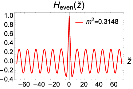
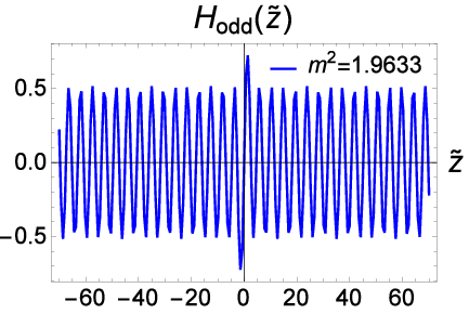
When the wave functions are either even-parity or odd-parity, the Schrödinger-like equation can be solved numerically. The dimensionless effective potential is expressed in terms of . Figure 6 shows the influence of on the effective potential and the resonant modes of gravity. The relative probability as a function of is obtained, and only the peak which satisfies represents a resonance mode.


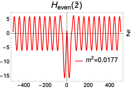
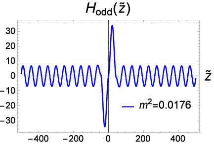
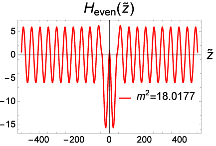
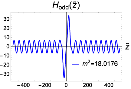
From Fig. 6, we see that, with the increasing of the parameter the effective potential splits from a single-well into a three-well potential, which indicates there are more resonant KK modes for larger , and this can be confirmed by Figs. 6(d), 6(e), 6(f). In Fig. 6(d), there are no peaks of the relative probability, which means there does not exist resonant mode. In Fig. 6(e), there is just one peak of the relative probability corresponding to the even-parity or the odd-parity wave function, and its wave functions with mass square and are plotted in Fig. 7, which shows that the resonance is indeed quasi-localized on the sub-brane. In Fig. 6(f), we find there are five peaks corresponding to the even-parity or the odd-parity resonant modes which satisfy , and the corresponding wave functions of the first even-parity and odd-parity modes with mass square and are plotted in Fig. 7. The numerical results of the mass spectrum, relative probability, full width at half maximum (FWHM) and lifetime of the resonance with are listed in Tab. 1. The resonances having a large lifetime can be quasi-localized on the brane for a long time. Note that the first even and odd resonance modes are not degenerate.
| parity | |||||||
|---|---|---|---|---|---|---|---|
| 0 | 1 | even | |||||
| 3 | 0 | 2 | odd | ||||
| 0 | 1 | odd | |||||
| 0 | 2 | even | |||||
| 0 | 3 | odd | |||||
| 0 | 4 | even | |||||
| 0 | 5 | odd | |||||
| 0 | 6 | even | |||||
| 8 | 0 | 7 | odd | ||||
| 0 | 8 | even | |||||
| 0 | 9 | odd | |||||
| 0 | 10 | even |
IV.2 Bent branes
Because the tensor perturbation of brane would not be stable, we now consider brane, which include two parameters and . Thus, the resonances are more involved and should be discussed specifically.


The effects of the parameters on the effective potentials and relative probability are shown in Fig. 8. The effective potentials have a multi-well with a minimum inside the brane and satisfy when . The effective potential does not change its shape but shift up and down with . Therefore, the number of the resonances, the relative probability , the width of mass , and the lifetime of the KK resonances do not change with for a fixed . Only the mass spectrum changes with . The specific values of masses of the resonances with different values of (including ) are listed in Tab. 2, from which we obtain that all of the masses of the resonances depend linearly on the parameter . For instance, the relations for the masses of the first even-parity and odd-parity modes with can be expressed as
| 28.8477 | ||||||||
| - | - | - | ||||||
| - | - | - | ||||||
| - | - | - | ||||||
| - | - | - | ||||||
| - | - | 18.3123 | - | |||||
| - | - | 18.3375 | - | 27.3375 | ||||
| - | - | - | - | - | - | 27.1745 | ||
| - | - | - | - | - | - | 27.1808 | ||
| (53) | |||||
| (54) |
We plot the fit functions for masses of the first even-parity and odd-parity modes with different in Fig. 9. The wave functions for the first even-parity and odd-parity modes with different are plotted in Fig. 10, which shows that the wave function does not alter with when is fixed.


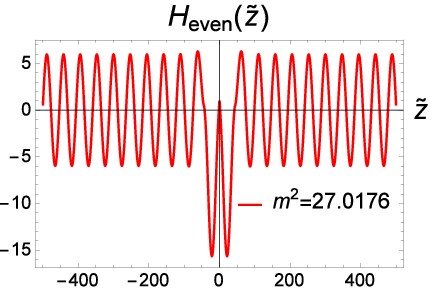
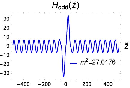
For brane, the potential well also becomes splitting, and the number of resonant modes increases with the parameter . The influence of the parameter on the effective potential and the probabilities is similar to flat brane, so we do not discuss it repeatedly. Here we list the numerical results for mass spectrum, the relative probability, the width of mass, and the lifetime of the KK resonances with different in Tab. 3.
| parity | |||||||
|---|---|---|---|---|---|---|---|
| -8 | 1 | even | |||||
| 3 | -8 | 2 | odd | ||||
| -8 | 1 | odd | |||||
| -8 | 2 | even | |||||
| -8 | 3 | odd | |||||
| -8 | 4 | even | |||||
| -8 | 5 | odd | |||||
| -8 | 6 | even | |||||
| 8 | -8 | 7 | odd | ||||
| -8 | 8 | even | |||||
| -8 | 9 | odd | |||||
| -8 | 10 | even |
V Conclusion
In this paper, we investigate the linear tensor perturbation for , and branes in two-field mimetic gravity. We apply the reconstruction technique to find a set of thick brane solutions in asymptotical space-time, and derive the master equations for linear tensor perturbations under the TT gauge condition. The Schrödinger-like equations for the and branes are factorized into a supersymmetric form; therefore, the brane systems are stable against the tensor perturbations, while the brane is unstable. For the flat and bent branes, the effective potentials of corresponding Schrödinger-like equation behave as volcano-like or modified-volcano-like potentials, which may allow a localized zero-mode responsible for the four-dimensional Newtonian potential and a series of massive resonant modes. The thick branes have two parameters and , one for the cosmological constant of the bent brane and the other for the inner structure of the domain wall. We investigate the effect of the two parameters on the thick branes, namely,
- •
when , the solution of changes into that of . In the limit , the bent brane solution is reduced to the flat brane solution. The number of the resonances does not change with ; however, the masses of resonant KK modes linearly decrease with the parameter for a fixed .
- •
as the parameter increases, the branes split into sub-branes, and the scalar field changes from a single-kink to a double-kink configuration; the effective potentials of the extra-dimensional parts of the tensor perturbations also split into multi-wells; the number of gravitational resonance modes increases.
Finally, we would like to point out that the tensor perturbation of the two-field mimetic gravity model is the same as that of the original single-field mimetic theory Yi2018 and GR. Nevertheless, the two mimetic scalar fields can generate different thick branes, leading to new types of effective potential and graviton resonant modes.
Acknowledgements
We sincerely thank Prof. Yu-Xiao Liu for helpful discussions. This work was supported by the National Natural Science Foundation of China (Grants No. 11705070) and the Fundamental Research Fund for Physics of Lanzhou University (No. Lzujbky-2019-ct06). Yi Zhong was supported by the Fundamental Research Funds for the Central Universities (Grants No. 531118010195).
References
- (1) N. Arkani-Hamed, S. Dimopoulos and G. R. Dvali, Phys. Lett. B 429 (1998), 263-272 [arXiv:hep-ph/9803315 [hep-ph]].
- (2) I. Antoniadis, N. Arkani-Hamed, S. Dimopoulos and G. R. Dvali, Phys. Lett. B 436 (1998), 257-263 [arXiv:hep-ph/9804398 [hep-ph]].
- (3) L. Randall and R. Sundrum, Phys. Rev. Lett. 83 (1999), 3370-3373 [arXiv:hep-ph/9905221 [hep-ph]].
- (4) L. Randall and R. Sundrum, Phys. Rev. Lett. 83 (1999), 4690-4693 [arXiv:hep-th/9906064 [hep-th]].
- (5) M. Gremm, Phys. Lett. B 478 (2000), 434-438 [arXiv:hep-th/9912060 [hep-th]].
- (6) O. DeWolfe, D. Z. Freedman, S. S. Gubser and A. Karch, Phys. Rev. D 62 (2000), 046008 [arXiv:hep-th/9909134 [hep-th]].
- (7) S. Kobayashi, K. Koyama and J. Soda, Phys. Rev. D 65 (2002), 064014 [arXiv:hep-th/0107025 [hep-th]].
- (8) D. Bazeia, L. Losano and C. Wotzasek, Phys. Rev. D 66 (2002), 105025 [arXiv:hep-th/0206031 [hep-th]].
- (9) A. Wang, Phys. Rev. D 66 (2002), 024024 [arXiv:hep-th/0201051 [hep-th]].
- (10) D. Bazeia and A. R. Gomes, JHEP 05 (2004), 012 [arXiv:hep-th/0403141 [hep-th]].
- (11) V. I. Afonso, D. Bazeia and L. Losano, Phys. Lett. B 634 (2006), 526-530 [arXiv:hep-th/0601069 [hep-th]].
- (12) D. Bazeia, F. A. Brito and L. Losano, JHEP 11 (2006), 064 [arXiv:hep-th/0610233 [hep-th]].
- (13) C. Bogdanos, A. Dimitriadis and K. Tamvakis, Phys. Rev. D 74 (2006), 045003 [arXiv:hep-th/0604182 [hep-th]].
- (14) V. Dzhunushaliev, V. Folomeev and M. Minamitsuji, Rept. Prog. Phys. 73 (2010), 066901 [arXiv:0904.1775 [gr-qc]].
- (15) Y. X. Liu, Y. Zhong and K. Yang, EPL 90 (2010) no.5, 51001 [arXiv:0907.1952 [hep-th]].
- (16) N. Barbosa-Cendejas and A. Herrera-Aguilar, JHEP 10 (2005), 101 [arXiv:hep-th/0511050 [hep-th]].
- (17) A. Herrera-Aguilar, D. Malagon-Morejon and R. R. Mora-Luna, JHEP 11 (2010), 015 [arXiv:1009.1684 [hep-th]].
- (18) Y. Zhong and Y. X. Liu, Eur. Phys. J. C 76 (2016) no.6, 321 [arXiv:1507.00630 [hep-th]].
- (19) V. A. Rubakov and M. E. Shaposhnikov, Phys. Lett. B 125 (1983), 139.
- (20) A. H. Chamseddine and V. Mukhanov, JHEP 11 (2013), 135 [arXiv:1308.5410 [astro-ph.CO]].
- (21) A. H. Chamseddine, V. Mukhanov and A. Vikman, JCAP 06 (2014), 017 [arXiv:1403.3961 [astro-ph.CO]].
- (22) E. A. Lim, I. Sawicki and A. Vikman, JCAP 05 (2010), 012 [arXiv:1003.5751 [astro-ph.CO]].
- (23) E. Babichev and S. Ramazanov, Phys. Rev. D 95 (2017) no.2, 024025 [arXiv:1609.08580 [gr-qc]].
- (24) N. Sadeghnezhad and K. Nozari, Phys. Lett. B 769 (2017), 134-140 [arXiv:1703.06269 [gr-qc]].
- (25) A. Casalino, M. Rinaldi, L. Sebastiani and S. Vagnozzi, Phys. Dark Univ. 22 (2018), 108 [arXiv:1803.02620 [gr-qc]].
- (26) A. Ganz, N. Bartolo, P. Karmakar and S. Matarrese, JCAP 01 (2019), 056 [arXiv:1809.03496 [gr-qc]].
- (27) Y. Zheng, L. Shen, Y. Mou and M. Li, JCAP 08 (2017), 040 [arXiv:1704.06834 [gr-qc]].
- (28) R. Myrzakulov, L. Sebastiani, S. Vagnozzi and S. Zerbini, Class. Quant. Grav. 33 (2016) no.12, 125005 [arXiv:1510.02284 [gr-qc]].
- (29) S. Vagnozzi, Class. Quant. Grav. 34 (2017) no.18, 185006 [arXiv:1708.00603 [gr-qc]].
- (30) A. Casalino, M. Rinaldi, L. Sebastiani and S. Vagnozzi, Class. Quant. Grav. 36 (2019) no.1, 017001 [arXiv:1811.06830 [gr-qc]].
- (31) O. Malaeb, Phys. Rev. D 91 (2015) no.10, 103526 [arXiv:1404.4195 [gr-qc]].
- (32) M. Chaichian, J. Kluson, M. Oksanen and A. Tureanu, JHEP 12 (2014), 102 [arXiv:1404.4008 [hep-th]].
- (33) K. Takahashi and T. Kobayashi, JCAP 11 (2017), 038 [arXiv:1708.02951 [gr-qc]].
- (34) Y. Zheng, Y. L. Zheng [arXiv:1810.03826 [gr-qc]].
- (35) L. Y. Shen, Y. L. Zheng and M. Z Li, JCAP 12 (2019), 026 [arXiv:1909.01248 [gr-qc]].
- (36) S. Nojiri and S. D. Odintsov, Mod. Phys. Lett. A 29 (2014) no.40, 1450211 [arXiv:1408.3561 [hep-th]].
- (37) S. Nojiri, S. D. Odintsov and V. K. Oikonomou, Phys. Rev. D 94 (2016) no.10, 104050 [arXiv:1608.07806 [gr-qc]].
- (38) S. Nojiri, S. D. Odintsov and V. K. Oikonomou, Class. Quant. Grav. 33 (2016) no.12, 125017 [arXiv:1601.07057 [gr-qc]].
- (39) S. D. Odintsov and V. K. Oikonomou, Phys. Rev. D 93 (2016) no.2, 023517 [arXiv:1511.04559 [gr-qc]].
- (40) S. D. Odintsov and V. K. Oikonomou, Annals Phys. 363 (2015) 503 [arXiv:1508.07488 [gr-qc]].
- (41) A. V. Astashenok, S. D. Odintsov and V. K. Oikonomou, Class. Quant. Grav. 32 (2015) no.18, 185007 [arXiv:1504.04861 [gr-qc]].
- (42) S. Nojiri, S. D. Odintsov and V. K. Oikonomou, Phys. Lett. B 775 (2017) 44 [arXiv:1710.07838 [gr-qc]].
- (43) G. Cognola, R. Myrzakulov, L. Sebastiani, S. Vagnozzi and S. Zerbini, Class. Quant. Grav. 33 (2016) no.22, 225014 [arXiv:1601.00102 [gr-qc]].
- (44) N. Hosseinkhan and K. Nozari, Eur. Phys. J. Plus 133 (2018) no.2, 50
- (45) W. D. Guo, Y. Zhong, K. Yang, T. T. Sui and Y. X. Liu, Phys. Lett. B 800 (2020), 135099 [arXiv:1805.05650 [hep-th]].
- (46) J. Chen, W. D. Guo and Y. X. Liu, [arXiv:2011.03927 [gr-qc]].
- (47) S. Davood Sadatian and A. Sepehri, Mod. Phys. Lett. A 34 (2019) no.21, 1950162
- (48) Y. Zhong, Y. Zhong, Y. P. Zhang and Y. X. Liu, Eur. Phys. J. C 78 (2018) no.1, 45 [arXiv:1711.09413 [hep-th]].
- (49) H. Firouzjahi, M. A. Gorji and S. A. Hosseini Mansoori, JCAP 07, 031 (2017) [arXiv:1703.02923 [hep-th]].
- (50) M. A. Gorji, S. A. Hosseini Mansoori and H. Firouzjahi, JCAP 01, 020 (2018) [arXiv:1709.09988 [astro-ph.CO]].
- (51) H. Firouzjahi, M. A. Gorji, S. A. Hosseini Mansoori, A. Karami and T. Rostami, JCAP 11 (2018), 046 [arXiv:1806.11472 [gr-qc]].
- (52) D. Bazeia, L. Losano and J. R. L. Santos, Phys. Lett. A 377 (2013), 1615-1620 [arXiv:1304.6904 [hep-th]].
- (53) M. Higuchi and S. Nojiri, Gen. Rel. Grav. 46 (2014) no.11, 1822 [arXiv:1402.1346 [hep-th]].
- (54) Y. X. Liu, K. Yang and Y. Zhong, JHEP 10 (2010), 069 [arXiv:0911.0269 [hep-th]].
- (55) Y. X. Liu, H. Guo, C. E. Fu and H. T. Li, Phys. Rev. D 84 (2011), 044033 [arXiv:1101.4145 [hep-th]].
- (56) S. Kobayashi, K. Koyama and J. Soda, Phys. Rev. D 65 (2002), 064014 [arXiv:hep-th/0107025 [hep-th]].
- (57) A. Karch and L. Randall, JHEP 05 (2001), 008 [arXiv:hep-th/0011156 [hep-th]].
- (58) Y. X. Liu, C. E. Fu, L. Zhao and Y. S. Duan, Phys. Rev. D 80 (2009), 065020 [arXiv:0907.0910 [hep-th]].
- (59) Y. X. Liu, J. Yang, Z. H. Zhao, C. E. Fu and Y. S. Duan, Phys. Rev. D 80 (2009), 065019 [arXiv:0904.1785 [hep-th]].
- (60) Y. Z. Du, L. Zhao, Y. Zhong, C. E. Fu and H. Guo, Phys. Rev. D 88 (2013), 024009 [arXiv:1301.3204 [hep-th]].
- (61) Q. Tan, W. D. Guo, Y. P. Zhang and Y. X. Liu, [arXiv:2008.08440 [gr-qc]].