∎
Cascade Attentive Dropout for Weakly Supervised Object Detection
Abstract
Weakly supervised object detection (WSOD) aims to classify and locate objects with only image-level supervision. Many WSOD approaches adopt multiple instance learning as the initial model, which is prone to converge to the most discriminative object regions while ignoring the whole object, and therefore reduce the model detection performance. In this paper, a novel cascade attentive dropout strategy is proposed to alleviate the part domination problem, together with an improved global context module. We purposely discard attentive elements in both channel and space dimensions, and capture the inter-pixel and inter-channel dependencies to induce the model to better understand the global context. Extensive experiments have been conducted on the challenging PASCAL VOC 2007 benchmarks, which achieve 49.8% mAP and 66.0% CorLoc, outperforming state-of-the-arts.
Keywords:
Weakly supervised object detection Convolutional neural network Dropout1 Introduction

Weakly Supervised Object Detection (WSOD) is attracting more and more attention in computer vision area in recent years. The training of a traditional object detector usually is based on a large amount of manually labeled data, while the labeling process is time-consuming, expensive, and inefficient. Weakly supervised object detection has come into being, which aims to solve this problem by training a detector with only image-level annotations instead of bounding boxes.
Most methods model WSOD as a multiple instance learning (MIL) problem, where each image is considered as a bag and the object proposals as instances. During the training process, the network iterates in the following two steps: (1) training an object classifier to compute the object score of each object proposal; (2) selecting the proposals with the highest score and their similar proposals based on IoU. The model is prone to learn only the most discriminative object features rather than comprehensive object features so that it will cause part domination shown in Figure 1. For example, in the case of a cat, the head may be more discriminative than the body in which appearance changes dramatically due to patterns. In this case, previous techniques can localize only the head, rather than the entire region.
Recent work have alleviated this problem by using context informationkantorov2016contextlocnet; wei2018ts2c, progressive refinementtang2018pcl; tang2017multiple; wan2019c, and smoothed loss functionswan2019c. For example, Contextlocnetkantorov2016contextlocnet built additive and contrastive guidance models to utilize their surrounding context feature to enhance localization performance. C-MILwan2019c divided the instances in the bag into multiple subsets, and defines corresponding smoother loss functions on the each subset to approximate the convex loss function.
Attention mechanism, which enables network to focus on the most informative views, has been proven effective in many fields, such as image classificationhu2018squeeze, image inpaintingyu2018generative, medical image segmentationsinha2019multi, etc. However, the mechanism hurts the object localization performance of WSOD because it focuses only on the most discriminative features. To address this issue, we propose a cascaded attentive dropout module (CADM) to inducing the network to learn less discriminative features for classification but meaningful features for object localization. Specifically, following channel attentive dropout, two complementary attentive branch are built and randomly selected to build spatial-attentive feature maps, where the one rewards the most discriminative features while the other punishes them via a designed attentive dropout strategy. A global context module (GCM), which uses sigmoid to enhance nonlinearity and perform feature fusion through element-wise multiplication and additions, also been introduced into the proposed network to obtain better global context information.
In summary, the main contributions of our work can be summarized as follows:
- 1)
An end-to-end weakly supervised object detection network is proposed, considering both network attention and global context information.
- 2)
A lightweight but effective cascade attentive dropout module is designed to help the network learn more comprehensive features rather than only discriminative features, which notably improve the accuracy of WSOD.
- 3)
An improved global context module is introduced to further boost the learned features in a more efficient way of feature fusion, jointly optimizing the region classification and localization.
- 4)
The proposed network significantly outperforms most state-of-the-art weakly supervised object detection approaches on PASCAL VOC 2007.
2 Related Work
2.1 Weakly supervised object detection
Recent work have combined MIL and CNN to train a weakly supervised object detector in an end-to-end way. Bilen and Vedaldibilen2016weakly proposed a two-stream weakly supervised deep detection network (WSDDN) to get classification and detection scores respectively. Based on WSDDN, Tang et al.tang2017multiple proposed an online instance classifier refinement (OICR) approach to refine the rough output of WSDDN, Kantorov et al.kantorov2016contextlocnet introduced two different kinds of context-aware guidance to improve localization performance of the network. Tang et al.tang2018pcl also proposed a graph-based center cluster method to alleviate the local optimum problem. Some work have also begun to link weak supervision and strong supervision to comprehensively solve the WSOD problem. Zhang et al.zhang2018w2f designed a Weakly-supervised to fully-supervised framework (W2F) which mines high-quality pseudo ground truth to train a fully-supervised object detector. Wang et al.wang2018collaborative proposed a weakly supervised collaborative learning approach that adopts WSDDN and Faster-RCNN as weakly and strongly supervised sub-network respectively. From the perspective of optimization, Wang et al.wan2019c introduce a continuation optimization method into MIL to boost the detection performance. Arun et al.arun2019dissimilarity designed a novel dissimilarity coefficient based WSOD framework which is optimized by minimizing the difference between an annotation agnostic prediction distribution and an annotation aware conditional distribution. Besides, some work combined the tasks of weakly supervised object detection and segmentation into a unified end-to-end learning architecturegao2019c; zeng2019wsod2.
2.2 Dropout
Dropout is a regularization technique originally proposed by hinton2012improving to alleviate the over-fitting problem of fully connected neural networks, which randomly drops neurons with fixed probability during network training. However, all neuron activations are retained while testing the model, and the final output will be scaled according to the dropout probability. In this way, the network can easily integrate several different small models to achieve good regularization. Inspired by Dropout, Dropconnectwan2013regularization, Monte Carlo dropoutgal2016dropout, and many others were also introduced. This is only useful for the fully connected layer, but useless for the convolution layer. One of the reasons may be that the spatially adjacent pixels on the feature map are related to each other and share contextual information. After that, DeVries et al.devries2017improved designed Cutout to randomly drop out contiguous regions of input images, Tompson et al.tompson2015efficient also proposed SpatialDropout to randomly drops partial channels of a feature map, rather than dropping the independent random pixels. Besides, ADLchoe2019attention was proposed to utilize the attention mechanism to erase the maximally activated part.

2.3 Attention mechanism
The Attention mechanism is inspired by the human vision which does not treat all data equally but enhances or weakens them. Recent work have been proposed to improve the localization performance of the model. For example, Hu et. al proposed a squeeze-and-excitation network (SENet)hu2018squeeze to model the inter-channel dependencies, which generates a weight of via a global average pooling layer and two FC layers and multiply it into the input feature map to get an enhanced feature map. Based on SENet, SKNetli2019selective built multiple branches of different receptive fields and used the information summarized by the multiple scale feature to channel-wise guide how to allocate the representation of which kernel to focus on. Wang et. al proposed Non-local Neural networks to fuse the global information and bring richer semantic information to the following layers. Convolutional Block Attention Module (CBAM)woo2018cbam are also proposed to enhance features in channel and spatial dimensions in a cascading manner.
3 The Proposed Approach
In this section, we will introduce our proposed weakly supervised object detection architecture. As shown in Figure 2, the first stage aims to extract enhanced feature maps from VGG16 with a cascade attentive dropout module (CADM) and a global context module (GCM). The enhanced feature maps and region proposals generated by Selective Searchuijlings2013selective are then sent to the RoI pooling layer to produce fixed-size RoI feature maps. At last, MIL Refinement Module utilizes proposal feature vectors to predict object categories and locations. The proposed CADM, which is designed to elliminate negative effects of discriminative features, is employed on pooling 3 feature map. Different from ADL[21] which erased the maximally activated spatial parts, we purposely discard attentive elements in both channel and space dimension. The remainder of this section will discuss these components in detail.

3.1 Cascade Attentive Dropout Module
Weakly supervised object detectors tend to learn only the most discriminative features in imageswan2018min; wan2019c, which will cause network localization errors and decrease detection accuracy. In order to solve this problem, we try to dropout elements in the dimensions of channel and space respectively, as shown in Figure 3.
Channel-Dropout. Given a feature map extracted from CNN, the channel-dropout module takes it as input and outputs a global information embedding via a global average pooling (GAP) layer. The embedding can also be considered as the confidence of different channels, denoted as . Note that is the mini-batch number, is the number of channel, and are weight and height of the feature map, respectively. After that, we refer the confidence of the channel with the highest confidence as , and set the threshold . When the channel confidence is greater than , the channel is dropped; otherwise, keep the channel. Consequently, a binary channel-dropout mask is generated to indicate whether each channel is dropped or not, as shown in formula 1.
| (1) |
where equal to 0 means the -th channel is dropped. The binary drop mask is then multiplied to input map to get the channel-dropped feature map :
| (2) |
where denotes broadcast element-wise multiplication.
Spatial-Dropout. A complementary symmetric structure is constructed for spatial dropout to induce the network to learn more comprehensive features. We first get the self-attention map via a channel-wise average pooling layer. Since the activation value of more discriminative areas in the attention map is higher, we set a threshold to erase these areas to force the network to learn less discriminative features for classification but meaningful features for object localization, thereby avoiding location part domination. For the self-attention map , the maximum value of row is recorded as . When the element in row and column of the attention map is greater than the corresponding drop threshold , the element is dropped; otherwise, the element is retained. As a result, we can obtain a binary spatial-dropout mask :
| (3) |
where equal to 0 means the element in row and column of should be discarded. When decreases, more element values will be discarded.
However, when applying spatial-dropout throughout the training peroid, the most discriminative elements will always be ignored. As a result, the classification performance of the network will also be significantly reduced, which will also harm localization performance. In order to make up for the reduction of classification ability, we set up a reward branch to further enhance the discriminative elements. Specifically, the proposed network activates the self-attention map through a sigmoid function to obtain an importance map , where the intensity of each pixel in the importance map is close to 1 for the most discriminative features and close to 0 for the least discriminative features. During the training process, the network stochastically chooses either of the drop mask or importance map according to , and the selected one is merged into the input feature map to gain the spatial-dropped feature by element-wise multiplication:
| (4) |
where is a random number from a uniform distribution on the interval [0, 1).

3.2 Global Context Module
The non-local strategywang2018non has been proved its efficiency on modeling long-distance dependencies of pixel pairs. NLNet wang2018non learns a position-independent attention map for each position, which is time-consuming. SENethu2018squeeze uses the global context to calibrate the weights of different channels to adjust the channel dependence, in which the weight calibration inhabits its use of global context. In the paper, a new global context module like GCNetcao2019gcnet is introduced to enhance the understanding of the global context in a more efficient way, as shown in Figure 4.
The module can be divided into three stages: global attention pooling, bottleneck transform, and feature fusion. At the first stage, we obtain the attention weights via convolutional layer and a softmax layer, and multiple it into the input to get the global context features , which is expected to help the model better understand the visual scene globally. After that, the model capture channel-wise dependencies through two convolutional layers . In order to reduce the difficulty of model optimization, a layer normalization (LN) is inserted into the module (before ReLU). Sigmoid activation is also employed to learn a non-matually-exclusive relationship to improve original bottleneck transform of GCNet. Finally, unlike GCNet, which uses element-wise addition to fuse features, our enhanced features are fused into the original input by element-wise multiplication and then addition.
Denoting and as the input and output feature map of the global context module,so this module can be formulated as :
| (5) |
| (6) |
where is the nonlinear activation function Sigmoid, and is the index of query positions, and and is the height and weight of the feature map. indicates the bottleneck transform to capture channel-wise dependencies.

3.3 MIL and Refinement Module
Following felipe2020distilling, we build three submodules to classify and optimize instances, as shown in Figure 5. The first module trains a basic multiple instance learning network, which branches the proposal feature vectors into two streams to get by two FC layers, where is the number of proposals. These two matrices are passed through a softmax layer on the classes and proposals dimensions respectively to get the activated prediction result . The predictions of the two branches are fused by element-wise multiplication to obtain the category prediction score of the region proposal. Finally, the prediction score of this image for class can be obtained by summing up the scores over proposal dimensions. We use multi-classes cross-entropy loss to guide the training of this submodule:
| (7) |
where indicates that the input image contain class object and otherwise.
The second submodule builds K instance classifiers to optimize the output of the basic instance classifier. Each classifier is implemented by a FC layer and a softmax layer along categories (background is considered as class). The output of the classifier is considered as the supervision information of the classifier. so we can train the refined instance classifier based on the loss function in formula 8.
| (8) |
where is the loss weight term of region proposal to reduce the noise of supervision and the same as tang2017multiple. is the pseudo grouth truth information for class from the classifier, and indicates the prediction score of region proposal for class in the refinement branch.
Finally, we average the outputs of the K refinements agents outputs as the supervision to guide the distillation agent, which consist of a single FC layer and a softmax layer over class dimension. The distillation loss is the same as the refinement loss . As a result, The final loss function of the entire network is as follows:
| (9) |
4 Experiments
In this section, we will first introduce the dataset we used and the implementation details of our proposed approach. Then we will explore the contributions of each proposed module by the ablation experiments. Finally, we will compare the performance of our proposed network with the-state-of-art methods.
4.1 Datasets and Evaluation Metrics
we evaluate our method on the challenging PASCAL VOC2007 datasetseveringham2010pascal which have 9963 images for 20 object classes and are divided into three subsets: training, verification, and testing sets. The trainval set (5011 images) is chosen to train our proposed network. As we focus on weakly-supervised detection, only image-level labels (presence or absence of a class in the chosen image)are utilized during training. For testing, we evaluating our network using mean average precision (mAP)everingham2010pascal and correct localization (CorLoc) metricsdeselaers2012weakly. All these metrics are based on the PASCAL criteria of IoU > 0.5 between ground truths and predicted boxes.
4.2 Implementation Details
We use Selective searchuijlings2013selective to generate original region proposal and build our proposed network on VGG16simonyan2014very pre-trained on ImageNetdeng2009imagenet. We add the CADM module to the back layer of pooling3. The last max-pooling layer is replaced by ROI pooling and the last FC layer and softmax loss layer are replaced by the layer described in Section 3.3. We insert the global context module in front of the ROI layer.
The original input images are resized into five different scales {480,576,688,864,1200} concerning the smallest image dimension. The resized scale of a training image is randomly selected and the image is randomly horizontal flipped. In this way, each image is augmented into a total of ten images as many other WSOD methods dotang2017multiple; tang2018pcl; wan2018min; wan2019c. During network learning, we employ the SGD algorithm with momentum 0.9, weight decay and batch size 4. The model iterates 50K iterations, where the learning rate is set to for the first 20K iterations and then decreases to in the following 30K iterations. During testing, all ten augmented images are passed into the network, and take the averages as the final outputs. Non-maximum suppression is applied to all prediction with the IoU threshlod set to 0.3. Our experiments are implemented based on PyTorch deep learning framework and a NVIDIA GTX 1080Ti GPU.
| Methods | aero | bike | bird | boat | bottle | bus | car | cat | chair | cow |
|---|---|---|---|---|---|---|---|---|---|---|
| Baselinefelipe2020distilling | 63.1 | 66.4 | 46.1 | 25.4 | 16.9 | 70.8 | 68.8 | 53.2 | 14.9 | 56.8 |
| + CADM | 64.6 | 64.7 | 53.1 | 33.1 | 23.2 | 70.4 | 70.6 | 22.2 | 22.1 | 64.1 |
| + GCM | 66.0 | 66.0 | 56.8 | 20.3 | 19.1 | 72.5 | 70.6 | 59.5 | 19.6 | 64.3 |
| + Both | 66.5 | 65.6 | 56.5 | 26.8 | 19.7 | 69.9 | 69.0 | 61.3 | 21.5 | 66.9 |
| Methods | table | dog | horse | mbike | person | plant | sheep | sofa | train | tv |
| Baselinefelipe2020distilling | 41.5 | 53.7 | 42.7 | 70.0 | 2.9 | 20.6 | 42.8 | 44.8 | 50.8 | 68.3 |
| + CADM | 46.2 | 27.1 | 49.3 | 70.8 | 2.6 | 19.5 | 57.1 | 55.3 | 64.6 | 69.9 |
| + GCM | 42.8 | 47.8 | 42.8 | 68.5 | 2.5 | 20.0 | 47.6 | 48.7 | 62.9 | 64.2 |
| + Both | 43.1 | 50.4 | 49.0 | 70.1 | 2.3 | 20.1 | 53.9 | 47.4 | 65.7 | 70.7 |
| Methods | aero | bike | bird | boat | bottle | bus | car | cat | chair | cow |
|---|---|---|---|---|---|---|---|---|---|---|
| Baselinefelipe2020distilling | 84.6 | 78.4 | 59.2 | 49.5 | 44.7 | 77.7 | 85.0 | 61.0 | 34.8 | 75.3 |
| + CADM | 84.6 | 77.6 | 70.6 | 56.4 | 50.4 | 78.7 | 84.4 | 39.0 | 47.9 | 82.9 |
| + GCM | 84.2 | 82.4 | 70.3 | 64.4 | 44.7 | 79.7 | 86.6 | 47.1 | 46.9 | 84.2 |
| + Both | 84.2 | 75.7 | 75.1 | 50.0 | 40.8 | 77.7 | 82.3 | 68.6 | 46.3 | 82.2 |
| Methods | table | dog | horse | mbike | person | plant | sheep | sofa | train | tv |
| Baselinefelipe2020distilling | 44.1 | 70.5 | 65.0 | 88.8 | 11.4 | 57.1 | 73.2 | 51.9 | 66.2 | 82.4 |
| + CADM | 52.1 | 38.4 | 70.4 | 90.4 | 10.8 | 55.7 | 81.4 | 69.4 | 78.7 | 82.1 |
| + GCM | 48.7 | 40.0 | 73.5 | 88.8 | 11.0 | 55.7 | 82.5 | 66.4 | 70.3 | 82.4 |
| + Both | 52.9 | 63.5 | 73.1 | 89.6 | 10.6 | 52.7 | 79.4 | 55.4 | 78.7 | 82.1 |
| Methods | mAP | CorLoc |
|---|---|---|
| Baselinefelipe2020distilling | 46.0 | 63.0 |
| + CADM | 47.5 | 65.1 |
| + GCM | 48.1 | 65.5 |
| + CADM + GCM | 49.8 | 66.0 |
| multiplication | addition | multiplication + addition | mAP |
| 46 | |||
| 47.8 | |||
| 47.0 | |||
| 48.1 |
| channel-dropout | spatial-dropout | channel + spatial dropout | mAP |
| 48.1 | |||
| 47.6 | |||
| 48.8 | |||
| 49.8 |
4.3 Ablation experiments
we conduct extensive ablation experiments on PASCAL VOC2007 to prove the effectiveness of our proposed network and respectively validate the contribution of each component including CADM and GCM.
4.3.1 Baseline
We use Boosted-OICRfelipe2020distilling as our baseline. We re-run the author’s code multiple times with the same configuration, but the highest mAP we can achieve is only 46.0% due to different cuda versions and GPUs. 11 1 More details about the issue can refer to https://github.com/ppengtang/pcl.pytorch/issues/9
4.3.2 GCM
We conduct experiments with and without GCM to illustrate the effectiveness of GCM and denote the network with GCM as +GCM, which does not include CADM and report the results in Table 1 , Table 2 and Table 3. The detection performance of 13 classes and the localization performance of 11 classes have been improved. Figure 3 shows that applying global context module to our proposed network could improve the performance of the model by at least 2.1% mAP and 2.5% CorLoc.
We also explore the effect of different way of feature fusion on model performance on PASCAL VOC 2007 and the results are shown in Table 4. It shows that multiplication and then addition is more effective than simple multiplication or addition in the fusion stage.

| Methods | aero | bike | bird | boat | bottle | bus | car | cat | chair | cow |
|---|---|---|---|---|---|---|---|---|---|---|
| WSDDNbilen2016weakly | 46.4 | 58.3 | 35.5 | 25.9 | 14.0 | 66.7 | 53.0 | 39.2 | 8.9 | 41.8 |
| DSTLjie2017deep | 52.2 | 47.1 | 35 | 26.7 | 15.4 | 61.3 | 66 | 54.3 | 3 | 53.6 |
| OICRtang2017multiple | 58.0 | 62.4 | 31.1 | 19.4 | 13.0 | 65.1 | 62.2 | 28.4 | 24.8 | 44.7 |
| WCCNdiba2017weakly | 49.5 | 60.6 | 38.6 | 29.2 | 16.2 | 70.8 | 56.9 | 42.5 | 10.9 | 44.1 |
| PCLtang2018pcl | 54.4 | 69.0 | 39.3 | 19.2 | 15.7 | 62.9 | 64.4 | 30.0 | 25.1 | 52.5 |
| TS2Cwei2018ts2c | 59.3 | 57.5 | 43.7 | 27.3 | 13.5 | 63.9 | 61.7 | 59.9 | 24.1 | 46.9 |
| C-WSLgao2018c | 62.7 | 63.7 | 40.0 | 25.5 | 17.7 | 70.1 | 68.3 | 38.9 | 25.4 | 54.5 |
| W2Fzhang2018w2f | 60.9 | 68.7 | 47.1 | 31.7 | 14.2 | 71.2 | 68.9 | 24.5 | 23.5 | 57.6 |
| WeakRPNtang2018weakly | 57.9 | 70.5 | 37.8 | 5.7 | 21.0 | 66.1 | 69.2 | 59.4 | 3.4 | 57.1 |
| BOICRfelipe2020distilling | 63.1 | 66.4 | 46.1 | 25.4 | 16.9 | 70.8 | 68.8 | 53.2 | 14.9 | 56.8 |
| MELMwan2018min | 55.6 | 66.9 | 34.2 | 29.1 | 16.4 | 68.8 | 68.1 | 43.0 | 25.0 | 65.6 |
| ZLDNzhang2018zigzag | 55.4 | 68.5 | 50.1 | 16.8 | 20.8 | 62.7 | 66.8 | 56.5 | 2.1 | 57.8 |
| WSCDNwang2018collaborative | 61.2 | 66.6 | 48.3 | 26.0 | 15.8 | 66.5 | 65.4 | 53.9 | 24.7 | 61.2 |
| C-MILwan2019c | 62.5 | 58.4 | 49.5 | 32.1 | 19.8 | 70.5 | 66.1 | 63.4 | 20.0 | 60.5 |
| Ours | 66.5 | 65.6 | 56.45 | 26.8 | 19.7 | 69.9 | 69.0 | 61.3 | 21.5 | 66.9 |
| Methods | table | dog | horse | mbike | person | plant | sheep | sofa | train | tv |
| WSDDNbilen2016weakly | 26.6 | 38.6 | 44.7 | 59.0 | 10.8 | 17.3 | 40.7 | 49.6 | 56.9 | 50.8 |
| DSTLjie2017deep | 24.7 | 43.6 | 48.4 | 65.8 | 6.6 | 18.8 | 51.9 | 43.6 | 53.6 | 62.4 |
| OICRtang2017multiple | 30.6 | 25.3 | 37.8 | 65.5 | 15.7 | 24.1 | 41.7 | 46.9 | 64.3 | 62.6 |
| WCCNdiba2017weakly | 29.9 | 42.2 | 47.9 | 64.1 | 13.8 | 23.5 | 45.9 | 54.1 | 60.8 | 54.5 |
| PCLtang2018pcl | 44.4 | 19.6 | 39.3 | 67.7 | 17.8 | 22.9 | 46.6 | 57.5 | 58.6 | 63.0 |
| TS2Cwei2018ts2c | 36.7 | 45.6 | 39.9 | 62.6 | 10.3 | 23.6 | 41.7 | 52.4 | 58.7 | 56.6 |
| C-WSLgao2018c | 41.6 | 29.9 | 37.9 | 64.2 | 11.3 | 27.4 | 49.3 | 54.7 | 61.4 | 67.4 |
| W2Fzhang2018w2f | 43.6 | 20.9 | 47.9 | 66.0 | 11.3 | 22.3 | 56.4 | 57.7 | 61.1 | 60.1 |
| WeakRPNtang2018weakly | 57.3 | 35.2 | 64.2 | 68.6 | 32.8 | 28.6 | 50.8 | 49.5 | 41.1 | 30.0 |
| BOICRfelipe2020distilling | 41.5 | 53.7 | 42.7 | 70 | 2.9 | 20.6 | 42.8 | 44.8 | 50.8 | 68.3 |
| MELMwan2018min | 45.3 | 53.2 | 49.6 | 68.6 | 2.0 | 25.4 | 52.5 | 56.8 | 62.1 | 57.1 |
| ZLDNzhang2018zigzag | 47.5 | 40.1 | 69.7 | 68.2 | 21.6 | 27.2 | 53.4 | 56.1 | 52.5 | 58.2 |
| WSCDNwang2018collaborative | 46.2 | 53.5 | 48.5 | 66.1 | 12.1 | 22.0 | 49.2 | 53.2 | 66.2 | 59.4 |
| C-MILwan2019c | 52.9 | 53.5 | 57.4 | 68.9 | 8.4 | 24.6 | 51.8 | 58.7 | 66.7 | 63.5 |
| Ours | 43.1 | 50.4 | 49.0 | 70.1 | 2.3 | 20.1 | 53.9 | 47.4 | 65.7 | 70.7 |
| Methods | aero | bike | bird | boat | bottle | bus | car | cat | chair | cow |
|---|---|---|---|---|---|---|---|---|---|---|
| WSDDNbilen2016weakly | 65.1 | 58.8 | 58.5 | 33.1 | 39.8 | 68.3 | 60.2 | 59.6 | 34.8 | 64.5 |
| DSTLjie2017deep | 72.7 | 55.3 | 53.0 | 27.8 | 35.2 | 68.6 | 81.9 | 60.7 | 11.6 | 71.6 |
| OICRtang2017multiple | 81.7 | 80.4 | 48.7 | 49.5 | 32.8 | 81.7 | 85.4 | 40.1 | 40.6 | 79.5 |
| WCCNdiba2017weakly | 83.9 | 72.8 | 64.5 | 44.1 | 40.1 | 65.7 | 82.5 | 58.9 | 33.7 | 72.5 |
| PCLtang2018pcl | 79.6 | 85.5 | 62.2 | 47.9 | 37.0 | 83.8 | 83.4 | 43.0 | 38.3 | 80.1 |
| TS2Cwei2018ts2c | 84.2 | 74.1 | 61.3 | 52.1 | 32.1 | 76.7 | 82.9 | 66.6 | 42.3 | 70.6 |
| C-WSLgao2018c | 86.3 | 80.4 | 58.3 | 50.0 | 36.6 | 85.8 | 86.2 | 47.1 | 42.7 | 81.5 |
| WeakRPNtang2018weakly | 77.5 | 81.2 | 55.3 | 19.7 | 44.3 | 80.2 | 86.6 | 69.5 | 10.1 | 87.7 |
| BOICRfelipe2020distilling | 84.6 | 78.4 | 59.2 | 49.5 | 44.7 | 77.7 | 85.0 | 61.0 | 34.8 | 75.3 |
| ZLDNzhang2018zigzag | 74.0 | 77.8 | 65.2 | 37.0 | 46.7 | 75.8 | 83.7 | 58.8 | 17.5 | 73.1 |
| WSCDNwang2018collaborative | 85.8 | 80.4 | 73.0 | 42.6 | 36.6 | 79.7 | 82.8 | 66.0 | 34.1 | 78.1 |
| ours | 84.2 | 75.7 | 75.1 | 50.0 | 40.8 | 77.7 | 82.3 | 68.6 | 46.3 | 82.2 |
| Methods | table | dog | horse | mbike | person | plant | sheep | sofa | train | tv |
| WSDDNbilen2016weakly | 30.5 | 43.0 | 56.8 | 82.4 | 25.5 | 41.6 | 61.5 | 55.9 | 65.9 | 63.7 |
| DSTLjie2017deep | 29.7 | 54.3 | 64.3 | 88.2 | 22.2 | 53.7 | 72.2 | 52.6 | 68.9 | 75.5 |
| OICRtang2017multiple | 35.7 | 33.7 | 60.5 | 88.8 | 21.8 | 57.9 | 76.3 | 59.9 | 75.3 | 81.4 |
| WCCNdiba2017weakly | 25.6 | 53.7 | 67.4 | 77.4 | 26.8 | 49.1 | 68.1 | 27.9 | 64.5 | 55.7 |
| PCLtang2018pcl | 50.6 | 30.9 | 57.8 | 90.8 | 27.0 | 58.2 | 75.3 | 68.5 | 75.7 | 78.9 |
| TS2Cwei2018ts2c | 39.5 | 57.0 | 61.2 | 88.4 | 9.3 | 54.6 | 72.2 | 60.0 | 65.0 | 70.3 |
| C-WSLgao2018c | 42.2 | 42.6 | 50.7 | 90.0 | 14.3 | 61.9 | 85.6 | 64.2 | 77.2 | 82.4 |
| WeakRPNtang2018weakly | 68.4 | 52.1 | 84.4 | 91.6 | 57.4 | 63.4 | 77.3 | 58.1 | 57.0 | 53.8 |
| BOICRfelipe2020distilling | 44.1 | 70.5 | 65.0 | 88.8 | 11.4 | 57.1 | 73.2 | 51.9 | 66.2 | 82.4 |
| ZLDNzhang2018zigzag | 49.0 | 51.3 | 76.7 | 87.4 | 30.6 | 47.8 | 75.0 | 62.5 | 64.8 | 68.8 |
| WSCDNwang2018collaborative | 36.9 | 68.6 | 72.4 | 91.6 | 22.2 | 51.3 | 79.4 | 63.7 | 74.5 | 74.6 |
| Ours | 52.9 | 63.5 | 73.1 | 89.6 | 10.6 | 52.7 | 79.4 | 55.4 | 78.7 | 82.1 |
4.3.3 CADM
To verify the effectiveness of CADM, we also conduct experiments with and without CADM. We empirically set original threshold to 0.8, to 0.8 and denote the network with GAM as +CADM, which does not include a global context module. From Table 1 , Table 2 and Table 3, we can conclude that CADM does help the detector learn comprehensive features rather than only discriminative features and brings at least 1.5% mAP and 2.1% CorLoc improvement.
We also further investigate the effect of different on detection performance, as shown in Figure 6. When exploring the role of a certain value, the other two values are fixed at 0.8. From the three subgraphs, we can find that different values have a greater impact on the performance of the model, sometimes it will greatly improve the performance of the model (49.8% vs 48.1%), but sometimes it will hurt the performance of the model (46.8% vs 48.1%). As a result, an appropriate threshold selection is very important.
From Table 5, we can find that using the spatial-dropout submodule can slightly improve the performance of the model, but simply using the channel-dropout submodule will damage the performance of the model to a certain extent. Interestingly, when both submodules are inserted into the network in a cascaded way, the performance of the model is greatly improved. We believe that this is because a simple channel-dropout submodule may throw away too many elements, and the increase in localization performance cannot make up for the loss of classification performance, thereby compromising the final accuracy. But when the two are combined, the more discriminative features are moderately discarded to induce the network to learn those less discriminative features, thereby greatly improving the performance of the model.
| Methods | mAP | CorLoc |
|---|---|---|
| WSDDN bilen2016weakly | 39.2 | 53.5 |
| DSTL jie2017deep | 41.7 | 56.1 |
| OICR tang2017multiple | 42.0 | 60.6 |
| WCCN diba2017weakly | 42.8 | 56.7 |
| PCL tang2018pcl | 43.5 | 62.7 |
| TS2C wei2018ts2c | 44.3 | 61.0 |
| C-WSL gao2018c | 45.6 | 63.3 |
| WSD+FSD1 zhang2018w2f | 45.8 | 65.0 |
| WeakRPN tang2018weakly | 45.3 | 63.8 |
| BOICR felipe2020distilling | 46.0 | 63.0 |
| MELM wan2018min | 47.3 | 61.4 |
| ZLDN zhang2018zigzag | 47.3 | 61.2 |
| WSCDN wang2018collaborative | 48.3 | 64.7 |
| C-MIL wan2019c | 50.3 | 65.0 |
| Ours | 49.8 | 66.0 |
| Methods | mAP | CorLoc |
|---|---|---|
| DSTL jie2017deep | 38.3 | 58.8 |
| OICR tang2017multiple | 37.9 | 62.1 |
| WCCN diba2017weakly | 37.9 | - |
| PCL tang2018pcl | 40.6 | 63.2 |
| TS2C wei2018ts2c | 40.0 | 64.4 |
| C-WSL gao2018c | 41.5 | 64.2 |
| WSD+FSD1 zhang2018w2f | 42.4 | 65.5 |
| WeakRPN tang2018weakly | 40.8 | 64.9 |
| MELM wan2018min | 42.4 | - |
| ZLDN zhang2018zigzag | 42.9 | 61.5 |
| WSCDN wang2018collaborative | 43.3 | 65.2 |
| C-MIL wan2019c | 46.6 | 67.4 |
| SDCN li2019weakly | 43.5 | 67.9 |
| BOICR felipe2020distilling | 46.7 | 66.3 |
| MIL-OICR+GAM+REG yang2019towards | 46.8 | 69.5 |
| Ours | 46.9 | 66.5 |
4.4 Comparison with state-of-the-art
Table 6 and Table 8 shows the detection performance of our proposed method and a comparison with other state-of-the-art methods on the PASCAL VOC 2007 test set. It can be seen that our proposed method improves the original Boosted-OICRfelipe2020distilling code in 3.8% mAP, and outperformed WSDDNbilen2016weakly, OICRtang2017multiple, WSCDNwang2018collaborative, MELMwan2018min and other approaches by 1.5% 10.6%. Meanwhile, our method achieved the highest AP results in 6 classes(aeroplane, bird, motorbike, cow, sheep and tv).
We also evaluated object location performance of our network and compared it with other SOTA on the PASCAL VOC 2007 trainval set in Table 7 and Table 8. The proposed network reached the best localization performance in 4 of the 20 classes(aeroplane, bird, chair and train). our network respectively outperformed WSDDNbilen2016weakly, OICRtang2017multiple, WSCDNwang2018collaborative, MELMwan2018min, C-MILwan2019c and other approaches by 1.0% 12.5%.
We achieve a performance of 46.9% mAP and 66.5% CorLoc on Pascal VOC 2012, which is supervior to previous work in with gain of about 0.1% 8.6% mAP in Table 9.
4.5 Visualization
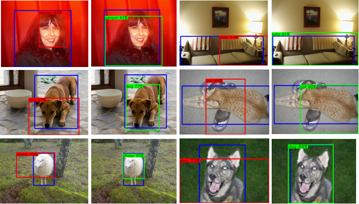
The visualization of our network and baselinefelipe2020distilling detection results is shown in Figure 7. The first and third columns are the detection results of felipe2020distilling, and the other two columns are our detection results. Our proposed methods have achieved better detection results than felipe2020distilling, and the part-dominated problem has been better alleviated as shown in the first two rows. As can be seen from the third row of pictures, our method can also improve the problem of too large a prediction box.
5 Conclusion
In this paper, we propose a simple but effective architecture for weakly supervised object detection. The network selectively discards the most discriminative features in the channel and spatial dimensions based on attention mechanism. To understand the image context information better, a global context module is also introduced into MIL. We have conducted extensive experiments and results show substantial and distinctive improvement of the our proposed method.
Acknowledgements.
This work is supported by the National Natural Science Foundation of China(grant no. 61573168)References
- (1) Kantorov, V., Oquab, M., Cho, M., Laptev, I.: Contextlocnet: Context-aware deep network models for weakly supervised localization. In: European Conference on Computer Vision, pp. 350–365. Springer (2016)
- (2) Wei, Y., Shen, Z., Cheng, B., Shi, H., Xiong, J., Feng, J., Huang, T.: Ts2c: Tight box mining with surrounding segmentation context for weakly supervised object detection. In: Proceedings of the European Conference on Computer Vision (ECCV), pp. 434–450 (2018)
- (3) Tang, P., Wang, X., Bai, S., Shen, W., Bai, X., Liu, W., Yuille, A.: Pcl: Proposal cluster learning for weakly supervised object detection. IEEE transactions on pattern analysis and machine intelligence 42(1), 176–191 (2018)
- (4) Tang, P., Wang, X., Bai, X., Liu, W.: Multiple instance detection network with online instance classifier refinement. In: Proceedings of the IEEE Conference on Computer Vision and Pattern Recognition, pp. 2843–2851 (2017)
- (5) Wan, F., Liu, C., Ke, W., Ji, X., Jiao, J., Ye, Q.: C-mil: Continuation multiple instance learning for weakly supervised object detection. In: Proceedings of the IEEE Conference on Computer Vision and Pattern Recognition, pp. 2199–2208 (2019)
- (6) Hu, J., Shen, L., Sun, G.: Squeeze-and-excitation networks. In: Proceedings of the IEEE conference on computer vision and pattern recognition, pp. 7132–7141 (2018)
- (7) Yu, J., Lin, Z., Yang, J., Shen, X., Lu, X., Huang, T.S.: Generative image inpainting with contextual attention. In: Proceedings of the IEEE conference on computer vision and pattern recognition, pp. 5505–5514 (2018)
- (8) Sinha, A., Dolz, J.: Multi-scale guided attention for medical image segmentation. arXiv preprint arXiv:1906.02849 (2019)
- (9) Bilen, H., Vedaldi, A.: Weakly supervised deep detection networks. In: Proceedings of the IEEE Conference on Computer Vision and Pattern Recognition, pp. 2846–2854 (2016)
- (10) Zhang, Y., Bai, Y., Ding, M., Li, Y., Ghanem, B.: W2f: A weakly-supervised to fully-supervised framework for object detection. In: Proceedings of the IEEE conference on computer vision and pattern recognition, pp. 928–936 (2018)
- (11) Wang, J., Yao, J., Zhang, Y., Zhang, R.: Collaborative learning for weakly supervised object detection. arXiv preprint arXiv:1802.03531 (2018)
- (12) Arun, A., Jawahar, C., Kumar, M.P.: Dissimilarity coefficient based weakly supervised object detection. In: Proceedings of the IEEE Conference on Computer Vision and Pattern Recognition, pp. 9432–9441 (2019)
- (13) Gao, Y., Liu, B., Guo, N., Ye, X., Wan, F., You, H., Fan, D.: C-midn: Coupled multiple instance detection network with segmentation guidance for weakly supervised object detection. In: Proceedings of the IEEE International Conference on Computer Vision, pp. 9834–9843 (2019)
- (14) Zeng, Z., Liu, B., Fu, J., Chao, H., Zhang, L.: Wsod2: Learning bottom-up and top-down objectness distillation for weakly-supervised object detection. In: Proceedings of the IEEE International Conference on Computer Vision, pp. 8292–8300 (2019)
- (15) Hinton, G.E., Srivastava, N., Krizhevsky, A., Sutskever, I., Salakhutdinov, R.R.: Improving neural networks by preventing co-adaptation of feature detectors. arXiv preprint arXiv:1207.0580 (2012)
- (16) Wan, L., Zeiler, M., Zhang, S., Le Cun, Y., Fergus, R.: Regularization of neural networks using dropconnect. In: International conference on machine learning, pp. 1058–1066 (2013)
- (17) Gal, Y., Ghahramani, Z.: Dropout as a bayesian approximation: Representing model uncertainty in deep learning. In: international conference on machine learning, pp. 1050–1059 (2016)
- (18) DeVries, T., Taylor, G.W.: Improved regularization of convolutional neural networks with cutout. arXiv preprint arXiv:1708.04552 (2017)
- (19) Tompson, J., Goroshin, R., Jain, A., LeCun, Y., Bregler, C.: Efficient object localization using convolutional networks. In: Proceedings of the IEEE conference on computer vision and pattern recognition, pp. 648–656 (2015)
- (20) Choe, J., Shim, H.: Attention-based dropout layer for weakly supervised object localization. In: Proceedings of the IEEE Conference on Computer Vision and Pattern Recognition, pp. 2219–2228 (2019)
- (21) Li, X., Wang, W., Hu, X., Yang, J.: Selective kernel networks (2019)
- (22) Woo, S., Park, J., Lee, J.Y., So Kweon, I.: Cbam: Convolutional block attention module. In: Proceedings of the European conference on computer vision (ECCV), pp. 3–19 (2018)
- (23) Uijlings, J.R., Van De Sande, K.E., Gevers, T., Smeulders, A.W.: Selective search for object recognition. International journal of computer vision 104(2), 154–171 (2013)
- (24) Wan, F., Wei, P., Jiao, J., Han, Z., Ye, Q.: Min-entropy latent model for weakly supervised object detection. In: Proceedings of the IEEE Conference on Computer Vision and Pattern Recognition, pp. 1297–1306 (2018)
- (25) Wang, X., Girshick, R., Gupta, A., He, K.: Non-local neural networks. In: Proceedings of the IEEE conference on computer vision and pattern recognition, pp. 7794–7803 (2018)
- (26) Cao, Y., Xu, J., Lin, S., Wei, F., Hu, H.: Gcnet: Non-local networks meet squeeze-excitation networks and beyond. In: Proceedings of the IEEE International Conference on Computer Vision Workshops, pp. 0–0 (2019)
- (27) Felipe Zeni, L., Jung, C.R.: Distilling knowledge from refinement in multiple instance detection networks. In: Proceedings of the IEEE/CVF Conference on Computer Vision and Pattern Recognition Workshops, pp. 768–769 (2020)
- (28) Everingham, M., Van Gool, L., Williams, C.K., Winn, J., Zisserman, A.: The pascal visual object classes (voc) challenge. International journal of computer vision 88(2), 303–338 (2010)
- (29) Deselaers, T., Alexe, B., Ferrari, V.: Weakly supervised localization and learning with generic knowledge. International journal of computer vision 100(3), 275–293 (2012)
- (30) Simonyan, K., Zisserman, A.: Very deep convolutional networks for large-scale image recognition. arXiv preprint arXiv:1409.1556 (2014)
- (31) Deng, J., Dong, W., Socher, R., Li, L.J., Li, K., Fei-Fei, L.: Imagenet: A large-scale hierarchical image database. In: 2009 IEEE conference on computer vision and pattern recognition, pp. 248–255. Ieee (2009)
- (32) Jie, Z., Wei, Y., Jin, X., Feng, J., Liu, W.: Deep self-taught learning for weakly supervised object localization. In: Proceedings of the IEEE Conference on Computer Vision and Pattern Recognition, pp. 1377–1385 (2017)
- (33) Diba, A., Sharma, V., Pazandeh, A., Pirsiavash, H., Van Gool, L.: Weakly supervised cascaded convolutional networks. In: Proceedings of the IEEE conference on computer vision and pattern recognition, pp. 914–922 (2017)
- (34) Gao, M., Li, A., Yu, R., Morariu, V.I., Davis, L.S.: C-wsl: Count-guided weakly supervised localization. In: Proceedings of the European Conference on Computer Vision (ECCV), pp. 152–168 (2018)
- (35) Tang, P., Wang, X., Wang, A., Yan, Y., Liu, W., Huang, J., Yuille, A.: Weakly supervised region proposal network and object detection. In: Proceedings of the European conference on computer vision (ECCV), pp. 352–368 (2018)
- (36) Zhang, X., Feng, J., Xiong, H., Tian, Q.: Zigzag learning for weakly supervised object detection. In: Proceedings of the IEEE Conference on Computer Vision and Pattern Recognition, pp. 4262–4270 (2018)
- (37) Li, X., Kan, M., Shan, S., Chen, X.: Weakly supervised object detection with segmentation collaboration. In: Proceedings of the IEEE International Conference on Computer Vision, pp. 9735–9744 (2019)
- (38) Yang, K., Li, D., Dou, Y.: Towards precise end-to-end weakly supervised object detection network. In: Proceedings of the IEEE International Conference on Computer Vision, pp. 8372–8381 (2019)