DoDNet: Learning to segment multi-organ and tumors
from multiple partially labeled datasets
Abstract
Due to the intensive cost of labor and expertise in annotating 3D medical images at a voxel level, most benchmark datasets are equipped with the annotations of only one type of organs and/or tumors, resulting in the so-called partially labeling issue. To address this, we propose a dynamic on-demand network (DoDNet) that learns to segment multiple organs and tumors on partially labeled datasets.
DoDNet consists of a shared encoder-decoder architecture, a task encoding module, a controller for generating dynamic convolution filters, and a single but dynamic segmentation head. The information of the current segmentation task is encoded as a task-aware prior to tell the model what the task is expected to solve. Different from existing approaches which fix kernels after training, the kernels in dynamic head are generated adaptively by the controller, conditioned on both input image and assigned task. Thus, DoDNet is able to segment multiple organs and tumors, as done by multiple networks or a multi-head network, in a much efficient and flexible manner. We have created a large-scale partially labeled dataset, termed MOTS, and demonstrated the superior performance of our DoDNet over other competitors on seven organ and tumor segmentation tasks. We also transferred the weights pre-trained on MOTS to a downstream multi-organ segmentation task and achieved state-of-the-art performance. This study provides a general 3D medical image segmentation model that has been pre-trained on a large-scale partially labelled dataset and can be extended (after fine-tuning) to downstream volumetric medical data segmentation tasks. The dataset and code are available at: https://git.io/DoDNet
1 Introduction

Automated segmentation of abdominal organs and tumors using computed tomography (CT) is one of the most fundamental yet challenging tasks in medical image analysis pang2020ctumorgan; kavur2020chaos. It plays a pivotal role in a variety of computer-aided diagnosis tasks, including lesion contouring, surgical planning, and 3D reconstruction. Constrained by the labor cost and expertise, it is hard to annotate multiple organs and tumors at voxel level in a large dataset. Consequently, most benchmark datasets were collected for the segmentation of only one type of organs andor tumors, and all task-irrelevant organs and tumors were annotated as the background (see Fig. 1). For instance, the LiTS dataset bilic2019liver only has annotations of the liver and liver tumors, and the KiTS dataset heller2019kits19 only provides annotations of kidneys and kidney tumors. These partially labeled datasets are distinctly different from the segmentation benchmarks in other computer vision areas, such as PASCAL VOC everingham2010pascal and Cityscapes cordts2016cityscapes, where multiple types of objects were annotated on each image. Therefore, one of the significant challenges facing multi-organ and tumor segmentation is the so-called partially labeling issue, i.e., how to learn the representation of multiple organs and tumors under the supervision of these partially annotated images.
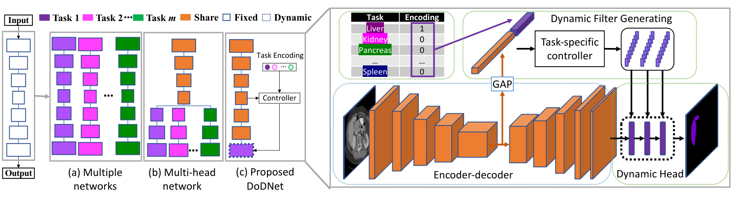
Mainstream approaches address this issue via separating the partially labeled dataset into several fully labeled subsets and training a network on each subset for a specific segmentation task yu2019crossbar; isensee2019automated; zhang2019light; myronenko20193d; zhu2019multi, resulting in ‘multiple networks’ shown in Fig. 2(a). Such an intuitive strategy, however, increases the computational complexity dramatically. Another commonly-used solution is to design a multi-head network (see Fig. 2(b)), which is composed of a shared encoder and multiple task-specific decoders (heads) chen2019med3d; fang2020multi; shi2020marginal. In the training stage, when each partially labeled data is fed to the network, only one head is updated and others are frozen. The inferences made by other heads are unnecessary and wasteful. Besides, the inflexible multi-head architecture is not easy to extend to a newly labeled task.
In this paper, we propose a dynamic on-demand network (DoDNet), which can be trained on partially labeled datasets for multi-organ and tumor segmentation. DoDNet is an encoder-decoder network with a single but dynamic head (see Fig. 2(c)), which is able to segment multiple organs and tumors as done by multiple networks or a multi-head network. The kernels in the dynamic head are generated adaptively by a controller, conditioned on the input image and assigned task. Specifically, the task-specific prior is fed to the controller to guide the generation of dynamic head kernels for each segmentation task. Owing to the light-weight design of the dynamic head, the computational cost of repeated inference can be ignored when compared to that of a multi-head network. We evaluate the effectiveness of DoDNet on seven organ and tumor segmentation benchmarks, involving the liver and tumors, kidneys and tumors, hepatic vessels and tumors, pancreas and tumors, colon tumors, and spleen. Besides, we transfer the weights pre-trained on partially labeled datasets to a downstream multi-organ segmentation task, and achieve state-of-the-art performance on the Multi-Atlas Labeling Beyond the Cranial Vault Challenge dataset. Our contributions are three-fold:
- •
We attempt to address the partially labeling issue from a new perspective, i.e., proposing a single network that has a dynamic segmentation head to segment multiple organs and tumors as done by multiple networks or a multi-head network.
- •
Different from the traditional segmentation head which is fixed after training, the dynamic segmentation head in our model is adaptive to the input and assigned task, leading to much improved efficiency and flexibility.
- •
The proposed DoDNet pre-trained on partially labeled datasets can be transferred to downstream annotation-limited segmentation tasks, and hence is beneficial for the medical community where only limited annotations are available for 3D image segmentation.
2 Related Work
Partially labeled medical image segmentation Segmentation of multiple organs and tumors is a generally recognized difficulty in medical image analysis Xie_multiorgan; zhang2020block; wang2019abdominal; schoppe2020deep, particularly when there is no large-scale fully labeled datasets. Although several partially labeled datasets are available, each of them is specialized for the segmentation of one particular organ andor tumors. Accordingly, a segmentation model is usually trained on one partially labeled dataset, and hence is only able to segment one particular organ and tumors, such as the liver and liver tumors li2018h; zhang2019light; seo2019modified; tang2020net, kidneys and kidney tumors myronenko20193d; Hou_kidney_isbi. Training multiple networks, however, suffers from the waste of computational resources and a poor scalability.
To address this issue, many attempts have been made to explore multiple partially labeled datasets in a more efficient manner. Chen et al. chen2019med3d collected multiple partially labeled datasets from different medical domains, and co-trained a heterogeneous 3D network on them, which is specially designed with a task-shared encoder and task-specific decoders for eight segmentation tasks. Huang et al. huang2020multi proposed to co-train a pair of weight-averaged models for unified multi-organ segmentation on few-organ datasets. Zhou et al. zhou2019prior first approximated anatomical priors of the size of abdominal organs on a fully labeled dataset, and then regularized the organ size distributions on several partially labeled datasets. Fang et al. fang2020multi treated the voxels with unknown labels as the background, and then proposed the target adaptive loss (TAL) for a segmentation network that is trained on multiple partially labeled datasets. Shi et al. shi2020marginal merged unlabeled organs with the background and imposed an exclusive constraint on each voxel (i.e. each voxel belongs to either one organ or the background) for learning a segmentation model jointly on a fully labeled dataset and several partially labeled datasets. To learn multi-class segmentation from single-class datasets, Dmitriev et al. dmitriev2019learning utilized the segmentation task as a prior and incorporated it into the intermediate activation signal.
The proposed DoDNet is different from these methods in three main aspects: (1) fang2020multi; shi2020marginal formulate the partially labeled issue as a multi-class segmentation task and treat unlabeled organs as the background, which may be misleading since the organ unlabeled in this dataset is indeed the foreground on another task. To address this issue, we formulate the partially labeled problem as a single-class segmentation task, aiming to segmenting each organ respectively; (2) Most of these methods adopt the multi-head architecture, which is composed of a shared backbone network and multiple segmentation heads for different tasks. Each head is either a decoder chen2019med3d or the last segmentation layer fang2020multi; shi2020marginal. In contrast, the proposed DoDNet is a single-head network, in which the head is flexible and dynamic; (3) Our DoDNet uses the dynamic segmentation head to address the partially labeled issue, instead of embedding the task prior into the encoder and decoder; (4) Most existing methods focus on multi-organ segmentation, while our DoDNet segments both organs and tumors, which is more challenging.
Dynamic filter learning Dynamic filter learning has drawn considerable research attention in the computer vision community due to its adaptive nature jia2016dynamic; yang2019condconv; chen2020dynamic; Tian2020CondInst; he2019dynamic; HDFNet_ECCV2020. Jia et al. jia2016dynamic designed a dynamic filter network, in which the filters are generated dynamically conditioned on the input. This design is more flexible than traditional convolutional networks, where the learned filters are fixed during the inference. Yang et al. yang2019condconv introduced the conditionally parameterized convolutions, which learn specialized convolutional kernels for each input, and effectively increase the size and capacity of a convolutional neural network. Chen et al. chen2020dynamic presented another dynamic network, which dynamically generates attention weights for multiple parallel convolution kernels and assembles these kernels to strengthen the representation capability. Pang et al. HDFNet_ECCV2020 integrated the features of RGB images and depth images to generate dynamic filters for better use of cross-modal fusion information in RGB-D salient object detection. Tian et al. Tian2020CondInst applied the dynamic convolution to instance segmentation, where the filters in the mask head are dynamically generated for each target instance. These methods successfully employ the dynamic filer learning towards certain ends, such as increasing the network flexibility jia2016dynamic, enhancing the representation capacity yang2019condconv; chen2020dynamic, integrating cross-modal fusion information HDFNet_ECCV2020, or abandoning the use of instance-wise ROIs Tian2020CondInst. Comparing to these works, our work here differs as follows. 1) we employ the dynamic filter learning to address the partially labeling issue for 3D medical image segmentation; and 2) the dynamic filters generated in our DoDNet are conditioned not only on the input image, but also on the assigned task.
3 Our Approach
3.1 Problem definition
Let us consider partially labeled datasets , which were collected for organ and tumor segmentation tasks:
Here, represents the -th partially labeled dataset that contains labeled images. The -th image in is denoted by , where is the size of each slice and is number of slices. The corresponding segmentation ground truth is , where the label of each voxel belongs to . Straightforwardly, this partially labeled multi-organ and tumor segmentation problem can be solved by training segmentation networks on datasets, respectively, shown as follows
| (1) |
where represents the loss function of each network, represent the parameters of these networks. In this work, we attempt to address this problem using only one single network , which can be formally expressed as
| (2) |
The DoDNet proposed here for this purpose consists of a shared encoder-decoder, a task encoding module, a dynamic filter generation module, and a dynamic segmentation head (see Fig. 2). We now delve into the details of each part.
3.2 Encoder-decoder architecture
The main component of DoDNet is the shared encoder-decoder that has an U-like architecture ronneberger2015u. The encoder is composed of repeated applications of 3D residual blocks he2016deep, each containing two convolutional layers with kernels. Each convolutional layer is followed by group normalization wu2018group and ReLU activation. At each downsampling step, the convolution with a stride of 2 is used to halve the resolution of input feature maps. The number of filters is set to 32 in the first layer, and is doubled after each downsampling step so as to preseve the time complexity per layer he2016deep. We totally perform four downsampling operations in the encoder. Given an input image , the output feature map is
| (3) |
where represents all encoder parameters.
Symmetrically, the decoder upsamples the feature map to improve its resolution and halve its channel number step by step. At each step, the upsampled feature map is first summed with the corresponding low-level feature map from the encoder, and then refined by a residual block. After upsampling the feature map four times, we have
| (4) |
where is the pre-segmentation feature map, represents all decoder parameters, and the channel number is set to 8 (see ablation study in Sec. 4.2).
The encoder-decoder aims to generate , which is supposed to be rich-semantic and not subject to a specific task, i.e., containing the semantic information of multiple organs and tumors.
3.3 Task encoding
Each partially labeled dataset contains the annotations of only a specific organ and related tumors. This information is a critical prior that tells the model with which task it is dealing and on which region it should focus. For instance, given an input sampled from the liver and tumor segmentation dataset, the proposed DoDNet is expected to be specialized for this task, i.e., predicting the masks of liver and liver tumors while ignoring other organs and other tumors. Intuitively, this task prior should be encoded into the model for task-awareness. Chen et al. chen2017fast encoded the task as a -dimensional one-hot vector, and concatenated the extended task encoding vector with the input image to form an augmented input. Owing to task encoding, the network ‘awares’ the task through the additional input channels and thus is able to accomplish multiple tasks, albeit with the performance degradation. However, the channel of input increases from to , leading to a dramatic increase of computation and memory cost. In this work, we also encode the task prior of each input into a -dimensional one-hot vector , shown as follows
| (5) |
Here, means that the annotation of -th task is available for the current input . Instead of extending the size of task encoding vector from to and using it as additional input channels chen2017fast, we first concatenate with the aggregated features and then use the concatenation for dynamic filter generation. Therefore, both computational and spatial complexity of our task encoding strategy is significantly lower than that in chen2017fast (see Figure 4).
3.4 Dynamic filter generation
For a traditional convolutional layer, the learned kernels are fixed after training and shared by all test cases. Hence, the network optimized on one task must be less-optimal to others, and it is hard to use a single network to perform multiple organ and tumor segmentation tasks. To overcome this difficulty, we introduce a dynamic filter method to generate the kernels, which are specialized to segment a particular organ and tumors. Specifically, a single convolutional layer is used as a task-specific controller . The image feature is aggregated via global average pooling (GAP) and concatenated with the task encoding vector as the input of . Then, the kernel parameters are generated dynamically conditioned not only on the assigned task but also on the input image itself, expressed as follows
| (6) |
where represents the controller parameters, and represents the concatenation operation.
| Conv layer | #Weights | #Bias |
|---|---|---|
| 1 | ||
| 2 | ||
| 3 | ||
| Totoal | ||
3.5 Dynamic head
During the supervised training, it is worthless to predict the organs and tumors whose annotations are not available. Therefore, a light-weight dynamic head is designed to enable specific kernels to be assigned to each task for the segmentation of a specific organ and tumors. The dynamic head contains three stacked convolutional layers with kernels. The kernel parameters in three layers, denoted by , are dynamically generated by the controller according to the input image and assigned task (see Eq. 6).
The first two layers have 8 channels, and the last layer has 2 channels, i.e., one channel for organ segmentation and the other for tumor segmentation. Therefore, a total of 162 parameters (see Table 1 for details) are generated by the controller. The partial predictions of -th image with regard to -th task is computed as
| (7) |
where represents the convolution, and represents the predictions of organs and tumors. Although each image requires a group of specific kernels for each task, the computation and memory cost of our light-weight dynamic head is negligible compared to the encoder-decoder (see Sec. 4.3).
3.6 Training and Testing
For simplicity, we treat the segmentation of an organ and related tumors as two binary segmentation tasks, and jointly use the Dice loss and binary cross-entropy loss as the objective for each task. The loss function is formulated as
| (8) | ||||
where and represent the prediction and ground truth of -th voxel, is the number of all voxels, and is added as a smoothing factor. We employ a simple strategy to train DoDNet on multiple partially labeled datasets, i.e., ignoring the predictions corresponding to unlabeled targets. Taking colon tumor segmentation for example, the result of organ prediction is ignored during the loss computation and error back-propagation, since the annotations of organs are unavailable.
During inference, the proposed DoDNet is flexible to segmentation tasks. Given a test image, the pre-segmentation feature is extracted from the encoder-decoder network. Assigned with a task, the controller generates the kernels conditioned on the input image and task. The dynamic head powered with the generated kernels is able to automatically segment the organ and tumors as specified by the task. In addition, if tasks are all required, our DoDNet is able to generate groups of kernels for the dynamic head and to efficiently segment all of organs and tumors in turn. Compared to the encoder-decoder, the dynamic head is so light that the inference cost of dynamic heads is almost negligible.
| Partial-label task | Annotations | # Images | ||
| Organ | Tumor | Training | Test | |
| #1 Liver | ✓ | ✓ | 104 | 27 |
| #2 Kidney | ✓ | ✓ | 168 | 42 |
| #3 Hepatic Vessel | ✓ | ✓ | 242 | 61 |
| #4 Pancreas | ✓ | ✓ | 224 | 57 |
| #5 Colon | ✓ | 100 | 26 | |
| #6 Lung | ✓ | 50 | 13 | |
| #7 Spleen | ✓ | 32 | 9 | |
| Total | - | - | 920 | 235 |
1.8in
| Depth | Average Dice | Average HD |
|---|---|---|
| 2 | 71.30 | 25.72 |
| 3 | 71.67 | 25.86 |
| 4 | 71.63 | 26.07 |
1.8in
| Width | Average Dice | Average HD |
|---|---|---|
| 4 | 69.79 | 30.40 |
| 8 | 71.67 | 25.86 |
| 16 | 71.45 | 26.31 |
| Image feat. | Task enc. | Average Dice | Average HD |
|---|---|---|---|
| ✓ | ✓ | 71.67 | 25.86 |
| ✓ | 71.26 | 29.38 | |
| ✓ | 51.80 | 79.94 |
4 Experiment
4.1 Experiment setup
Dataset: We built a large-scale partially labeled Multi-Organ and Tumor Segmentation (MOTS) dataset using multiple medical image segmentation benchmarks, including LiTSbilic2019liver, KiTS heller2019kits19, and Medical Segmentation Decathlon (MSD) simpson2019large. MOTS is composed of seven partially labeled sub-datasets, involving seven organ and tumor segmentation tasks. There are 1155 3D abdominal CT scans collected from various clinical sites around the world, including 920 scans for training and 235 for test. More details are given in Table 2. Each scan is re-sliced to the same voxel size of .
The MICCAI 2015 Multi Atlas Labeling Beyond the Cranial Vault (BCV) dataset BCV_benchmark was also used for this study. It is composed of 50 abdominal CT scans,including 30 scans for training and 20 for test. Each training scan is paired with voxel-wise annotations of 13 organs, including the liver, spleen, pancreas, right kidney, left kidney, gallbladder, esophagus, stomach, aorta, inferior vena cava, portal vein and splenic vein, right adrenal gland, and left adrenal gland. This dataset provides a downstream task, on which the segmentation network pre-trained on MOTS was evaluated.
Evaluation metric: The Dice similarity coefficient (Dice) and Hausdorff distance (HD) were used as performance metrics for this study. Dice measures the overlapping between a segmentation prediction and ground truth, and HD evaluates the quality of segmentation boundaries by computing the maximum distance between the predicted boundaries and ground truth.
Implementation details: All experiments were performed on a workstation with two NVIDIA 2080Ti GPUs. To filter irrelevant regions and simplify subsequent processing, we truncated the HU values in each scan to the range and linearly normalized them to . Owing to the benefits of group normalization wu2018group, our model adopts the micro-batch training strategy with a small batch size of 2. To accelerate the training process, we also employed the weight standarization qiao2019weight that smooths the loss landscape by standardizing the convolutional kernels. The stochastic gradient descent (SGD) algorithm with a momentum of 0.99 was adopted as the optimizer. The learning rate was initialized to 0.01 and decayed according to a polynomial policy , where the maximum epoch was set to 1,000. In the training stage, we randomly extracted sub-volumes with the size of from CT scans as the input. In the test stage, we employed the sliding window based strategy and let the window size equal to the size of training patches. To ensure a fair comparison, the same training strategies, including the weight standarization, learning rate, optimizer, and other settings, were applied to all competing models.
4.2 Ablation study
We split the 20% of training scans as validation data to perform the ablation study, which investigates the effectiveness of the detailed design of the dynamic head and dynamic filter generation module. We average the Dice score and HD of 11 organs and tumors (listed in Table 2) as two evaluation indicators for a fair comparison.
Depth of dynamic head: In Table 5, we compared the performance of the dynamic head with different depths, varying from 2 to 4. The width is fixed to 8, except for the last layer, which has 2 channels. It shows that, considering the trade-off between Dice and HD, DoDNet achieves the best performance on the validation set when the depth of dynamic head is set to 3. But the performance fluctuation is very small when the depth increases from 2 to 4. The results indicate the robustness of dynamic head to the varying depth. We empirically set the depth to 3 for this study.
Width of dynamic head: In Table 5, we compared the performance of the dynamic head with different widths, varying from 4 to 16. The depth is fixed to 3. It shows that the performance improves substantially when increasing the width from 4 to 8, but drops slightly when further increasing the width from 8 to 16. It suggest that the performance of DoDNet tends to become stable when the width of dynamic head falls within reasonable range (). Considering the complexity issue, we empirically set the width of dynamic head to 8.
Condition analysis: The kernels of dynamic head are generated on condition of both the input image and assigned task. We compared the effectiveness of both conditions in Table 5. It reveals that the task encoding plays a much more important role than image features in dynamic filer generation. It may be attributed to the fact that the task prior is able to make DoDNet aware of what task is being handled. Without the task condition, all kinds of organs, like liver, kidneys, and pancreas, are equally treated as the same foreground. In this case, it is hard for DoDNet to fit such a complex foreground that is composed of multiple organs. Moreover, DoDNet fails to distinguish each specific organ or tumors from this foreground without the task condition.
| Methods | Task 1: Liver | Task 2: Kidney | Task 3: Hepatic Vessel | |||||||||
|---|---|---|---|---|---|---|---|---|---|---|---|---|
| Dice | HD | Dice | HD | Dice | HD | |||||||
| Organ | Tumor | Organ | Tumor | Organ | Tumor | Organ | Tumor | Organ | Tumor | Organ | Tumor | |
| Multi-Nets | 96.61 | 61.65 | 4.25 | 41.16 | 96.52 | 74.89 | 1.79 | 11.19 | 63.04 | 72.19 | 13.73 | 50.70 |
| TAL fang2020multi | 96.18 | 60.82 | 5.99 | 38.87 | 95.95 | 75.87 | 1.98 | 15.36 | 61.90 | 72.68 | 13.86 | 43.57 |
| Multi-Head chen2019med3d | 96.75 | 64.08 | 3.67 | 45.68 | 96.60 | 79.16 | 4.69 | 13.28 | 59.49 | 69.64 | 19.28 | 79.66 |
| Cond-NO | 69.38 | 47.38 | 37.79 | 109.65 | 93.32 | 70.40 | 8.68 | 24.37 | 42.27 | 69.86 | 93.35 | 70.34 |
| Cond-Input chen2017fast | 96.68 | 65.26 | 6.21 | 47.61 | 96.82 | 78.41 | 1.32 | 10.10 | 62.17 | 73.17 | 13.61 | 43.32 |
| Cond-Dec dmitriev2019learning | 95.27 | 63.86 | 5.49 | 36.04 | 95.07 | 79.27 | 7.21 | 8.02 | 61.29 | 72.46 | 14.05 | 65.57 |
| DoDNet | 96.87 | 65.47 | 3.35 | 36.75 | 96.52 | 77.59 | 2.11 | 8.91 | 62.42 | 73.39 | 13.49 | 53.56 |
| Methods | Task 4: Pancreas | Task 5: Colon | Task 6: Lung | Task 7: Spleen | Average score | |||||||
| Dice | HD | Dice | HD | Dice | HD | Dice | HD | Dice | HD | |||
| Organ | Tumor | Organ | Tumor | Tumor | Tumor | Tumor | Tumor | Organ | Organ | |||
| Multi-Nets | 82.53 | 58.36 | 9.23 | 26.13 | 34.33 | 103.91 | 54.51 | 53.68 | 93.76 | 2.65 | 71.67 | 28.95 |
| TAL fang2020multi | 81.35 | 59.15 | 9.02 | 21.07 | 48.08 | 66.42 | 61.85 | 39.92 | 93.01 | 3.10 | 73.35 | 23.56 |
| Multi-Head chen2019med3d | 83.49 | 61.22 | 6.40 | 18.66 | 50.89 | 59.00 | 64.75 | 34.22 | 94.01 | 3.86 | 74.55 | 26.22 |
| Cond-NO | 65.31 | 46.24 | 36.06 | 76.26 | 42.55 | 76.14 | 57.67 | 102.92 | 59.68 | 38.11 | 60.37 | 61.24 |
| Cond-Input chen2017fast | 82.53 | 61.20 | 8.09 | 31.53 | 51.43 | 44.18 | 60.29 | 58.02 | 93.51 | 4.32 | 74.68 | 24.39 |
| Cond-Dec dmitriev2019learning | 77.24 | 55.69 | 17.60 | 48.47 | 51.80 | 63.67 | 57.68 | 53.27 | 90.14 | 6.52 | 72.71 | 29.63 |
| DoDNet | 82.64 | 60.45 | 7.88 | 15.51 | 51.55 | 58.89 | 71.25 | 10.37 | 93.91 | 3.67 | 75.64 | 19.50 |
4.3 Comparing to state-of-the-art methods
We compared the proposed DoDNet to state-of-the-art methods, which also attempt to address the partially labeling issue, on seven partially labeled tasks using the MOTS test set. The competitors include (1) seven individual networks, each being trained on a partially dataset (denoted by Multi-Nets), (2) two multi-head networks (i.e., Multi-Head chen2019med3d and TAL fang2020multi), (3) a single-network method without the task condition (Cond-NO), and (4) two single-network methods with the task condition (i.e., Cond-Input chen2017fast and Cond-Dec dmitriev2019learning). To ensure a fair comparison, we used the same encoder-decoder architecture for all methods, except that the channels of decoder layers in Multi-Head were halved due to GPU memory limitation.
Table 6 shows the performance metrics for the segmentation of each organ tumor and the average scores over 11 categories. It reveals that (1) most of methods (TAL, Multi-Head, Cond-Input, Cond-dec, DoDNet) achieve better performance than seven individual networks (Multi-Nets), suggesting that training with more data (even partially labelled) is beneficial to model performance; (2) Cond-NO fails to segment multiple organs and tumors when the task condition is unavailable, demonstrating the importance of task condition for a single network to address the partially labeling issue (consistent with the observation in Table 5); (3) the dynamic filter generation strategy is superior to directly embedding the task condition into the input or decoder (used in Cond-Input and Cond-Dec); and (4) the proposed DoDNet achieves the highest overall performance with an averaged Dice of 75.64% and an averaged HD of 19.50.
To make a qualitative comparison, we visualized the segmentation results obtained by six methods on seven tasks in Figure 3. It shows that our DoDNet outperforms other methods, especially in segmenting small tumors.
In Figure 4, we also compared the speed-accuracy trade-off of five methods. Single-network methods, including TAL, Cond-Dec, Cond-Input, and DoDNet, share the encoder and decoder for all tasks, and hence have a similar number of parameters, i.e., 17.3M. Although our DoDNet has an extra controller, the number of parameters in it is negligible. The Multi-Head network has a little more parameters (i.e., 18.9M) due to the use of multiple task-specific decoders. Multi-Nets has to train seven networks to address these partially labeled tasks, resulting in seven times more parameters than a single network.
As for inference speed, Cond-Input, Multi-Nets, Multi-Head, and Cond-Dec suffer from the repeated inference processes, and hence need more time to segment seven kinds of organ and tumors than other methods. In contrast, TAL is much more efficient to segment all targets, since the encoder-decoder (excepts for the last segmentation layer) is shared by all tasks. Our DoDNet shares the encoder-decoder architecture and specializes the dynamic head for each partially labeled task. Due to the light-weight architecture, the inference of dynamic head is very fast. In summary, our DoDNet achieves the best accuracy and a fast inference speed.

4.4 MOTS Pre-training for downstream tasks
Although achieving startling success driven by large-scale labeled data, deep learning remains trammelled by the limited annotations in medical image analysis. The largest partially labeled dataset, i.e., #3 Hepatic Vessel, only contains 242 training cases, which is much smaller than MOTS with 920 training cases. It has been generally recognized that training a deep model with more data contributes to a better generalization ability zoph2020rethinking; he2019rethinking; tran2018closer; esteva2017dermatologist. Therefore, pre-training a model on MOTS should be beneficial for the annotation-limited downstream task. To demonstrate this, we treated the BCV multi-organ segmentation as a downstream task and conducted experiments on the BCV dataset. We initialized the segmentation network, which has the same encoder-decoder structure as introduced in Sec. 3.2, using three initialization strategies, including randomly initialization (i.e., training from scratch), pre-training on the #3 Hepatic Vessel dataset, and pre-training on MOTS.
First, we split 20 cases from the BCV training set for validation, since the annotations of BCV test set were withheld for online assessment, which is inconvenient. Figure 5 shows the training loss and validation performance of the segmentation network with three initialization strategies. The validation performance is measured by the averaged Dice score calculated over 13 categories. It revels that, comparing to training from scratch, pre-training the network helps it converge quickly and perform better, particularly in the initial stage. Moreover, pre-training on a small dataset (i.e., #3 Hepatic Vessel) only slightly outperforms training from scratch, but pre-training on MOTS, which is much larger than #3 Hepatic Vessel, achieves not only the fastest convergence, but also a remarkable performance boost. The results demonstrate the strong generalization ability of the model pre-trained on MOTS.
Second, we also evaluated the effectiveness of the MOTS pre-trained weights on the BCV unseen test set. We compared our method to other state-of-the-art methods in Table 7, including Auto Context roth2018multi, DLTK pawlowski2017dltk, PaNN zhou2019prior, and nnUnet isensee2019automated. Comparing to training from scratch, using the MOTS pre-trained weights contributes to a substantial performance gain, improving the average Dice from 85.30% to 86.44%, reducing the average mean surface distance (SD) from 1.46 to 1.17, and reducing the average HD from 19.67 to 15.62. With the help of MOTS pre-training weights, our method achieves the best SD and HD, and second highest Dice on the test set.

| Methods | Avg. Dice | Avg. SD | Avg. HD |
|---|---|---|---|
| Auto Context roth2018multi | 78.24 | 1.94 | 26.10 |
| DLTK pawlowski2017dltk | 81.54 | 1.86 | 62.87 |
| PaNN zhou2019prior | 84.97 | 1.45 | 18.47 |
| nnUnet isensee2019automated | 88.10 | 1.39 | 17.26 |
| TFS | 85.30 | 1.46 | 19.67 |
| MOTS | 86.44 | 1.17 | 15.62 |
5 Conclusion
In this paper, we proposed DoDNet, a single encoder-decoder network with a dynamic head, to address the partially labelling issue for multi-organ and tumor segmentation in abdominal CT scans. We created a large-scale partially labeled dataset called MOTS and conducted extensive experiments on it. Our results indicate that, thanks to task encoding and dynamic filter learning, the proposed DoDNet achieves not only the best overall performance on seven organ and tumor segmentation tasks, but also higher inference speed than other competitors. We also demonstrated the value of DoDNet and the MOTS dataset by successfully transferring the weights pre-trained on MOTS to downstream tasks for which only limited annotations are available. It suggests that the byproduct of this work (i.e., a pre-trained 3D network) is conducive to other small-sample 3D medical image segmentation tasks.
References
- (1) Patrick Bilic, Patrick Ferdinand Christ, Eugene Vorontsov, et al. The liver tumor segmentation benchmark (LiTS). arXiv preprint arXiv:1901.04056, 2019.
- (2) Qifeng Chen, Jia Xu, and Vladlen Koltun. Fast image processing with fully-convolutional networks. In Proc. IEEE Int. Conf. Comp. Vis., pages 2497–2506, 2017.
- (3) Sihong Chen, Kai Ma, and Yefeng Zheng. Med3D: Transfer learning for 3D medical image analysis. arXiv preprint arXiv:1904.00625, 2019.
- (4) Yinpeng Chen, Xiyang Dai, Mengchen Liu, Dongdong Chen, Lu Yuan, and Zicheng Liu. Dynamic convolution: Attention over convolution kernels. In Proc. IEEE Conf. Comp. Vis. Patt. Recogn., pages 11030–11039, 2020.
- (5) Marius Cordts, Mohamed Omran, Sebastian Ramos, Timo Rehfeld, Markus Enzweiler, Rodrigo Benenson, Uwe Franke, Stefan Roth, and Bernt Schiele. The cityscapes dataset for semantic urban scene understanding. In Proc. IEEE Conf. Comp. Vis. Patt. Recogn., pages 3213–3223, 2016.
- (6) Konstantin Dmitriev and Arie E Kaufman. Learning multi-class segmentations from single-class datasets. In Proc. IEEE Conf. Comp. Vis. Patt. Recogn., pages 9501–9511, 2019.
- (7) Andre Esteva, Brett Kuprel, Roberto A Novoa, Justin Ko, Susan M Swetter, Helen M Blau, and Sebastian Thrun. Dermatologist-level classification of skin cancer with deep neural networks. Nature, 542(7639):115–118, 2017.
- (8) Mark Everingham, Luc Van Gool, Christopher KI Williams, John Winn, and Andrew Zisserman. The pascal visual object classes (VOC) challenge. Int. J. Comput. Vis., 88(2):303–338, 2010.
- (9) Xi Fang and Pingkun Yan. Multi-organ segmentation over partially labeled datasets with multi-scale feature abstraction. IEEE Trans. Med. Imaging, early access, 2020.
- (10) Junjun He, Zhongying Deng, and Yu Qiao. Dynamic multi-scale filters for semantic segmentation. In Proc. IEEE Int. Conf. Comp. Vis., pages 3562–3572, 2019.
- (11) Kaiming He, Ross Girshick, and Piotr Dollár. Rethinking imagenet pre-training. In Proc. IEEE Int. Conf. Comp. Vis., pages 4918–4927, 2019.
- (12) Kaiming He, Xiangyu Zhang, Shaoqing Ren, and Jian Sun. Deep residual learning for image recognition. In Proc. IEEE Conf. Comp. Vis. Patt. Recogn., pages 770–778, 2016.
- (13) Nicholas Heller, Niranjan Sathianathen, et al. The kits19 challenge data: 300 kidney tumor cases with clinical context, CT semantic segmentations, and surgical outcomes. arXiv preprint arXiv:1904.00445, 2019.
- (14) X. Hou, C. Xie, F. Li, J. Wang, C. Lv, G. Xie, and Y. Nan. A triple-stage self-guided network for kidney tumor segmentation. In IEEE Int. Sym. Biomed. Imaging, pages 341–344, 2020.
- (15) Rui Huang, Yuanjie Zheng, Zhiqiang Hu, Shaoting Zhang, and Hongsheng Li. Multi-organ segmentation via co-training weight-averaged models from few-organ datasets. In Proc. Int. Conf. Med. Image Comput. Comput.-Assist. Intervent., pages 146–155. Springer, 2020.
- (16) Fabian Isensee, Paul F Jäger, Simon AA Kohl, Jens Petersen, and Klaus H Maier-Hein. Automated design of deep learning methods for biomedical image segmentation. arXiv preprint arXiv:1904.08128, 2019.
- (17) Xu Jia, Bert De Brabandere, Tinne Tuytelaars, and Luc V Gool. Dynamic filter networks. In Proc. Adv. Neural Inf. Process. Syst., pages 667–675, 2016.
- (18) A Emre Kavur, N Sinem Gezer, Mustafa Barış, Pierre-Henri Conze, Vladimir Groza, Duc Duy Pham, Soumick Chatterjee, Philipp Ernst, Savaş Özkan, Bora Baydar, et al. Chaos challenge–combined (CT-MR) healthy abdominal organ segmentation. arXiv preprint arXiv:2001.06535, 2020.
- (19) Bennett Landman, Z Xu, JE Igelsias, M Styner, TR Langerak, and A Klein. Multi-atlas labeling beyond the cranial vault-workshop and challenge, 2017.
- (20) Xiaomeng Li, Hao Chen, Xiaojuan Qi, Qi Dou, Chi-Wing Fu, and Pheng-Ann Heng. H-denseunet: hybrid densely connected unet for liver and tumor segmentation from ct volumes. IEEE Trans. Med. Imaging, 37(12):2663–2674, 2018.
- (21) Andriy Myronenko and Ali Hatamizadeh. 3D kidneys and kidney tumor semantic segmentation using boundary-aware networks. arXiv preprint arXiv:1909.06684, 2019.
- (22) Shuchao Pang, Anan Du, Mehmet A Orgun, Zhenmei Yu, Yunyun Wang, Yan Wang, and Guanfeng Liu. Ctumorgan: a unified framework for automatic computed tomography tumor segmentation. Eur. J. Nucl. Med. Mol. Imaging, pages 1–21, 2020.
- (23) Youwei Pang, Lihe Zhang, Xiaoqi Zhao, and Huchuan Lu. Hierarchical dynamic filtering network for rgb-d salient object detection. In Proc. Eur. Conf. Comp. Vis., 2020.
- (24) Nick Pawlowski, Sofia Ira Ktena, Matthew CH Lee, Bernhard Kainz, Daniel Rueckert, Ben Glocker, and Martin Rajchl. DLTK: State of the art reference implementations for deep learning on medical images. arXiv preprint arXiv:1711.06853, 2017.
- (25) Siyuan Qiao, Huiyu Wang, Chenxi Liu, Wei Shen, and Alan Yuille. Weight standardization. arXiv preprint arXiv:1903.10520, 2019.
- (26) Olaf Ronneberger, Philipp Fischer, and Thomas Brox. U-net: Convolutional networks for biomedical image segmentation. In Proc. Int. Conf. Med. Image Comput. Comput.-Assist. Intervent., pages 234–241. Springer, 2015.
- (27) Holger R Roth, Chen Shen, Hirohisa Oda, Takaaki Sugino, Masahiro Oda, Yuichiro Hayashi, Kazunari Misawa, and Kensaku Mori. A multi-scale pyramid of 3D fully convolutional networks for abdominal multi-organ segmentation. In Proc. Int. Conf. Med. Image Comput. Comput.-Assist. Intervent., pages 417–425. Springer, 2018.
- (28) Oliver Schoppe, Chenchen Pan, Javier Coronel, Hongcheng Mai, Zhouyi Rong, Mihail Ivilinov Todorov, Annemarie Müskes, Fernando Navarro, Hongwei Li, Ali Ertürk, et al. Deep learning-enabled multi-organ segmentation in whole-body mouse scans. Nat. Commun., 11(1):1–14, 2020.
- (29) Hyunseok Seo, Charles Huang, Maxime Bassenne, Ruoxiu Xiao, and Lei Xing. Modified u-net (mu-net) with incorporation of object-dependent high level features for improved liver and liver-tumor segmentation in ct images. IEEE Trans. Med. Imaging, 39(5):1316–1325, 2019.
- (30) Gonglei Shi, Li Xiao, Yang Chen, and S Kevin Zhou. Marginal loss and exclusion loss for partially supervised multi-organ segmentation. arXiv preprint arXiv:2007.03868, 2020.
- (31) Amber L Simpson, Michela Antonelli, Spyridon Bakas, Michel Bilello, Keyvan Farahani, Bram Van Ginneken, Annette Kopp-Schneider, Bennett A Landman, Geert Litjens, Bjoern Menze, et al. A large annotated medical image dataset for the development and evaluation of segmentation algorithms. arXiv preprint arXiv:1902.09063, 2019.
- (32) Youbao Tang, Yuxing Tang, Yingying Zhu, Jing Xiao, and Ronald M Summers. E2Net: An edge enhanced network for accurate liver and tumor segmentation on ct scans. In Proc. Int. Conf. Med. Image Comput. Comput.-Assist. Intervent., pages 512–522. Springer, 2020.
- (33) Zhi Tian, Chunhua Shen, and Hao Chen. Conditional convolutions for instance segmentation. In Proc. Eur. Conf. Comp. Vis., 2020.
- (34) Du Tran, Heng Wang, Lorenzo Torresani, Jamie Ray, Yann LeCun, and Manohar Paluri. A closer look at spatiotemporal convolutions for action recognition. In Proc. IEEE Conf. Comp. Vis. Patt. Recogn., pages 6450–6459, 2018.
- (35) Yan Wang, Yuyin Zhou, Wei Shen, Seyoun Park, Elliot K Fishman, and Alan L Yuille. Abdominal multi-organ segmentation with organ-attention networks and statistical fusion. Med. Image Anal., 55:88–102, 2019.
- (36) Yuxin Wu and Kaiming He. Group normalization. In Proc. Eur. Conf. Comp. Vis., pages 3–19, 2018.
- (37) Lingxi Xie, Qihang Yu, Yuyin Zhou, Yan Wang, Elliot K. Fishman, and Alan L. Yuille. Recurrent saliency transformation network for tiny target segmentation in abdominal CT scans. IEEE Trans. Medical Imaging, 39(2):514–525, 2020.
- (38) Brandon Yang, Gabriel Bender, Quoc V Le, and Jiquan Ngiam. Condconv: Conditionally parameterized convolutions for efficient inference. In Proc. Adv. Neural Inf. Process. Syst., pages 1307–1318, 2019.
- (39) Qian Yu, Yinghuan Shi, Jinquan Sun, Yang Gao, Jianbing Zhu, and Yakang Dai. Crossbar-net: A novel convolutional neural network for kidney tumor segmentation in CT images. IEEE Trans. Image Process., 28(8):4060–4074, 2019.
- (40) Jianpeng Zhang, Yutong Xie, Pingping Zhang, Hao Chen, Yong Xia, and Chunhua Shen. Light-weight hybrid convolutional network for liver tumor segmentation. In Proc. Int. Joint Conf. Artificial Intelligence, pages 4271–4277, 2019.
- (41) Liang Zhang, Jiaming Zhang, Peiyi Shen, Guangming Zhu, Ping Li, Xiaoyuan Lu, Huan Zhang, Syed Afaq Shah, and Mohammed Bennamoun. Block level skip connections across cascaded v-net for multi-organ segmentation. IEEE Trans. Med. Imaging, 39(9):2782–2793, 2020.
- (42) Yuyin Zhou, Zhe Li, Song Bai, Chong Wang, Xinlei Chen, Mei Han, Elliot Fishman, and Alan L Yuille. Prior-aware neural network for partially-supervised multi-organ segmentation. In Proc. IEEE Int. Conf. Comp. Vis., pages 10672–10681, 2019.
- (43) Zhuotun Zhu, Yingda Xia, Lingxi Xie, Elliot K Fishman, and Alan L Yuille. Multi-scale coarse-to-fine segmentation for screening pancreatic ductal adenocarcinoma. In Proc. Int. Conf. Med. Image Comput. Comput.-Assist. Intervent., pages 3–12. Springer, 2019.
- (44) Barret Zoph, Golnaz Ghiasi, Tsung-Yi Lin, Yin Cui, Hanxiao Liu, Ekin Dogus Cubuk, and Quoc Le. Rethinking pre-training and self-training. In Proc. Adv. Neural Inf. Process. Syst., 2020.