CLIPPER: A Graph-Theoretic Framework for Robust Data Association
Abstract
We present CLIPPER (Consistent LInking, Pruning, and Pairwise Error Rectification), a framework for robust data association in the presence of noise and outliers. We formulate the problem in a graph-theoretic framework using the notion of geometric consistency. State-of-the-art techniques that use this framework utilize either combinatorial optimization techniques that do not scale well to large-sized problems, or use heuristic approximations that yield low accuracy in high-noise, high-outlier regimes. In contrast, CLIPPER uses a relaxation of the combinatorial problem and returns solutions that are guaranteed to correspond to the optima of the original problem. Low time complexity is achieved with an efficient projected gradient ascent approach. Experiments indicate that CLIPPER maintains a consistently low runtime of 15 ms where exact methods can require up to 24 s at their peak, even on small-sized problems with 200 associations. When evaluated on noisy point cloud registration problems, CLIPPER achieves 100% precision and 98% recall in 90% outlier regimes while competing algorithms begin degrading by 70% outliers. In an instance of associating noisy points of the Stanford Bunny with 990 outlier associations and only 10 inlier associations, CLIPPER successfully returns 8 inlier associations with 100% precision in 138 ms. Code is available at https://mit-acl.github.io/clipper.
I INTRODUCTION
Finding correct one-to-one correspondences between two sets of objects and is a fundamental problem in robotics, arising in a wide range of perception and estimation pipelines. In practice, observations of objects are “noisy” and “partial”, i.e., when an unknown number of objects in do not correspond to any object in (outliers). The traditional linear assignment approach based on corresponding objects of high similarity, e.g., using the Hungarian [1] or auction [2] algorithms, is not robust to high-noise, high-outlier regimes, leading to incorrect correspondences. In this work, we propose the CLIPPER (Consistent LInking, Pruning, and Pairwise Error Rectification) framework which leverages the notion of geometric consistency between object pairs to find correct correspondences in these extreme regimes. Our primary motivation is robust perception with applications such as those shown in Fig. 1, SLAM/loop closure [3, 4], point cloud registration [5, 6], shape alignment [7], object detection [8], and multiple object tracking [9, 10]. However, our framework is general and applicable to other pairwise data association problems.
When an attribute between objects in set is the same as the attribute between their correctly associated objects in , these objects are considered geometrically consistent (e.g., see Fig. 2). Incorporating geometric consistency in data association ultimately leads to a combinatorial optimization, such as maximum clique [11], maximum consensus [12, 13], or quadratic assignment [14] formulations. Relaxations of this NP-hard problem exist [15, 16], but exhibit poor performance in high-outlier regimes or for large problem size. In contrast, CLIPPER maintains high precision with low runtime across various outlier-regimes and problem sizes.
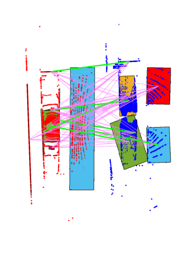
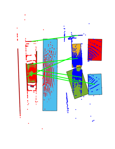
CLIPPER incorporates the concept of geometric consistency in a graph-theoretic framework, and proposes finding consistent association (inliers) by finding the densest subgraph. This formulation is particularly suited to weighted graphs and improves precision compared to maximum clique frameworks which are limited to binary graphs. CLIPPER uses the continuous relaxation technique introduced in [18] to guarantee that the recovered solution corresponds to a dense subgraph. Using projected gradient ascent with backtracking line search, CLIPPER achieves a consistently low runtime as compared to other algorithms. Further, our experiments show that CLIPPER is capable of attaining 100% precision even in high outlier regimes where other algorithms breakdown.
In summary, the contributions of this work include:
- •
An optimization formulation for selecting inlier associations suitable for both binary and weighted graphs.
- •
A relaxation of the resulting NP-hard optimization problem with optimality guarantees (see Sec III-A).
- •
A polynomial-time algorithm for solving the relaxed formulation based on projected gradient ascent, scalable to large-sized data association problems.
Additionally, we include a discussion on the application of geometric consistency to various observation types (e.g., points, lines, planes) commonly found in robotic perception. Finally, we benchmark CLIPPER against the state of the art when finding associations between two point clouds. We find that CLIPPER is able to achieve 100% precision in 99% outlier regimes, where the performance of competing algorithms begin to degrade.
Related works most pertinent to this work include Bailey et al. [11], where geometric consistency is leveraged for 2D LiDAR scan matching. Formulated as a maximum common subgraph problem, their technique resulted in a binary consistency graph for which the maximum clique indicated the correct data association. Leordeanu and Hebert [15] built on this graph-theoretic idea and instead constructed a weighted consistency graph, where edge weights represent the geometric consistency of associations. Enqvist et al. [19] noted the suboptimality of [15] and proposed a vertex covering formulation, essentially an alternative to the maximum clique formulation of [11]. Parra et al. [20] proposed a practical maximum clique algorithm for geometric consistency based on branch and bound and graph coloring. Recent algorithms leveraging these ideas for estimation tasks include PCM [4], where maximum cliques correspond to the largest set of pairwise-consistent loop closure measurements, and TEASER [6], where maximum cliques correspond to inlier associations for point cloud registration, further formalized in ROBIN [21]. CLIPPER advances these works with a continuous relaxation applicable to weighted graphs.

II Graph-Theoretic Formulation
A standard approach for robust data association in the presence of noise and outliers is to find the largest set of geometrically consistent associations. This problem can be formulated in a graph-theoretic framework. In this section, we review the consistency graph framework and the construction of the affinity matrix.
II-A Consistency Graph
For simplicity, and without loss of generality, we introduce the concept of a consistency graph for the point cloud registration problem. In Section V, we will show how this general framework can be used for robust data association in other robotic perception domains. The point cloud registration problem consists of finding the rotation and translation that map coordinates of a set of points to their corresponding points in another set. The main challenge is finding the correct correspondences as the points are noisy and contain outliers. Outlier points are points with large noise, and ones that are partially observed (i.e., points in one set that do no have a counterpart in the other set). Outlier associations are correspondences that match (inlier or outlier) points in one set incorrectly to points in the other set. Fig. 2a gives an example of two point clouds identified by blue and red colors. Inlier points are denoted by in the blue point cloud and their transformed counterparts by in the red point cloud. Points do not correspond to any blue point and hence are considered as outliers. A set of putative associations between the points, denoted by , are given, where are inlier and are outlier associations. In the case that no putative associations are given, an all-to-all hypothesis can be generated.
The consistency of associations can be assessed and represented in the graph-theoretic framework of the consistency graph. The consistency graph of associations consists of vertices, where each vertex represents an association. Edges between the vertices of show that their corresponding associations are consistent. The example in Fig. 2b illustrates the consistency graph for the associations in Fig. 2a. Since rotation and translation are distance-preserving transformations, the distance between the points in one set should be identical (in the noiseless setting) to their counterparts in the other set when associations are correct. This attribute can be used to assess the geometric consistency of two associations, where an edge between two vertices of indicates that the distances between the points matched by the associations are the same. The largest set of mutually consistent associations is given by the largest fully connected subgraph (maximum clique), which consists of vertices in the example of Fig. 2b.
II-B Affinity Matrix
The affinity matrix of a consistency graph with vertices is an symmetric matrix with entries in the interval . The diagonal entries measure the similarity of the data points that association matches, e.g., based on the similarity of point “descriptors” (for instance, the FPFH descriptors for point clouds [22]). Scores of and indicate the lowest and the highest similarity, respectively. The diagonal entries of are set to when similarity information is not available. In this case, , where is the (weighted) adjacency matrix of the consistency graph and is the identity matrix. The off-diagonal entries measure the geometric consistency of association pairs and , and similarly range from to . For example, in the point cloud registration problem, the distance between two points matched to by associations and can be used to measure the consistency as . Here, is a scoring function such that and for , as illustrated in Fig 2c. The threshold is based on a bounded noise model with a noise range of on the point coordinates. Hence, if the distance between the points differs more than this threshold, the associations are considered inconsistent. Another source of inconsistency, referred to as the distinctness constraint, is when correct associations are expected to be one-to-one. Hence, for any two associations and that originate or terminate at the same point, to indicate mutual inconsistency of associations. Lastly, we note that a binary scoring function, e.g., in Fig. 2c, can be used. This will lead to a binary affinity matrix, shown in Fig. 2d.
III Optimization Formulation of CLIPPER
Given the consistency graph with vertices representing associations (all-to-all or putative), and its , symmetric affinity matrix , we propose the problem
for finding the densest subset of consistent associations. Here, the optimization variable is a binary vector of size , with elements indicating associations that are selected as inliers, and ’s otherwise. Since is binary, the constraint ensures that if , then at most one of the associations or is selected in the answer.
When is binary (e.g., obtained by using the scoring function in Fig. 2c) and has one diagonal entries, it is straightforward to show that (III) simplifies to
Problem (III) is known as the maximum clique problem (MCP), and its solution gives the largest set of consistent associations. The MCP framework is used frequently in the literature [6, 4, 11] for data association in the presence of noise and a large number of outliers, where the vertices/associations in the maximum clique are considered as the correct/inlier correspondences. The justification for this consideration is based on the assumption that the noise and outlier points are random, unbiased, and unstructured, thus they are not expected to form a large clique in the consistency graph [15]. We note that MCP is a well-known NP-hard problem [23] in its full generality, hence, algorithms that rely on solving (III) become computationally intractable as the problem size grows.
The density of a graph is defined as the total sum of edge weights divided by the number of vertices. The densest subgraph is the subset of graph vertices and their corresponding edges that have the highest density. Given a graph with affinity matrix (with 1 diagonal entries), the densest subgraph of is found from
where elements in the solution correspond to the vertices in the densest subgraph [24]. Noting the similarity of the objectives in (III) and (III), problem (III) can be interpreted as finding the densest, fully connected subgraph of . The full connectivity requirement is due to the constraints in (III), which prohibit the selection of vertices that are not connected, i.e., . The densest-subgraph objective in (III) is crucial in the weighted case, and sets it apart from the maximum edge weighted clique problem [25]. For example, consider a weighted matrix and two solution candidates as
| (6) |
The MCP objective in (III), or the unnormalized objective of , returns as the optimum solution, whereas the block of corresponding to has low consistency scores of between the vertices/associations. On the other hand, the normalized objective of (III) takes values of and for and , respectively, leading to selection of the smaller, but more consistent subgraph. Example (6) further highlights the importance of choosing a weighted scheme over binary in the affinity matrix, since the maximum clique formulation returns as a solution. While this problem can be avoided by choosing a smaller , a conservative threshold leads to classifying correct associations as outliers (i.e., lower output recall). Further, a weighted scheme can resolve symmetric cases where two binary cliques have the same size.
III-A Continuous Relaxation
The main challenges in solving (III) are the combinatorial complexity of the problem due to its binary domain and the nonlinearity of the objective in . This makes it intractable to solve the problem to global optimality in real time, even for small-sized data association problems. A standard workaround is to relax the domain and the constraints of (III) to obtain a continuous problem amenable to fast solution, followed by projecting this solution back to the domain and constraint manifold of the original problem. Among the relaxation strategies that can be considered, the main advantage of the following approach is that the solutions obtained from the relaxed problem correspond to optima of the original problem, as will be discussed shortly.
We propose the relaxation of (III) as
where is the set of non-negative reals, is the vector norm, and
where is a positive scalar. This approach is inspired by [18], which directly integrates the constraints of the original problem into the continuous formulation of (III-A) via the matrix . Intuitively, when , the scalar penalizes joint selection of in the objective by the amount . Hence, as increases the entries of solution that violate the constraints are pushed to zero.
When , (local or global) optima of (III-A) satisfy the constraints in the original problem, i.e., if . This fact has been shown in [18] for the case when is a binary matrix. While we have extended the proof to the weighted case, this discussion is beyond the space constraints of this paper and will be presented in a subsequent journal submission. We remark that since (III) is an NP-hard problem, depending on the initial condition an optimization algorithm used for solving (III-A) may converge to a local optima. To guarantee finding the global optima, it would be required to search the entire space of solutions.
Given a solution of (III-A) with , let represent the subgraph that corresponds to the nonzero elements of , and be the submatrix of that corresponds to . Noting that , and therefore , satisfies the constraints in (III), problem (III) reduces to binarizing such that the objective is maximized. This is equivalent to the densest subgraph problem of (III), where the goal is to find that has the maximum density. The densest subgraph problem can be solved in polynomial time using existing algorithms [26], but a good approximate answer can be obtained immediately by selecting the largest elements of as vertices of . The justification follows from the well-known facts that , which is the spectral radius of , is a tight upper bound for the graph’s density [27] and nonzero elements of , which form the principal eigenvector of , represent centrality of their corresponding vertices, which is a measure of connectivity for a vertex in the graph [28].
IV CLIPPER Algorithm
The CLIPPER algorithm consists of 1) obtaining a solution of (III-A) via a projected gradient ascent approach with backtracking line search; and 2) estimating the densest cluster in by selecting the largest elements.
Algorithm 1 seeks a feasible subgraph by incrementally increasing the penalty parameter (Line 13) and solving (III-A) via gradient ascent (Lines 7-12). Noting that any optimal solution lies on the boundary of , the constraint manifold can be reduced to , where is the unit sphere. Instead of moving directly along the gradient , we first project onto the tangent space of at (Line 9) and move according to this orthogonal projection . To move quickly in the search space, the step size is chosen greedily so that if there is a to be penalized (i.e., and ), a gradient step would cause to hit the boundary of the positive orthant (Line 10). If no such exists, then is set such that the gradient update step gracefully degrades into a power iteration. In either case, if is chosen too large, backtracking line search is used to find an appropriate step (Line 11). The solution is projected back onto the constraint manifold (Line 12) and gradient ascent continues. Once has converged for the current value of , is incrementally increased (Line 13) and gradient ascent runs again with new objective . This process continues until and has converged. The convergence of the algorithm is guaranteed by the convergence property of the projected gradient approach [29].
The final step of CLIPPER selects the densest component of the subgraph (Lines 14-15), as explained in Section III-A. Since for all elements in the solution satisfy , then . The vertices of the densest component are then identified as the largest elements of .
IV-A Computational Considerations
Neglecting constant factors, the computational cost of Algorithm 1 is per iteration, where is the number of edges in the graph . Note that the orthogonal projection in Line 9 should be implemented as , which costs operations, where is the number of vertices in the graph . Most of the time is spent computing the matrix-vector product . All other operations run in at most operations.
V Constructing The Consistency Graph for Common Robotics Applications
CLIPPER can be applied to a broad array of data association problems found in robotics. All that is required is to identify a geometric invariant in the data, i.e., a quantity that is invariant under transformation. This invariant feature is then used to score geometric consistency for which a consistency graph can be constructed and CLIPPER can be used to quickly remove outlier associations. We briefly review how to score geometric consistency for the application examples in Fig. 1.
Point Clouds In Section II-A we described how two points seen in each cloud will have the same pairwise distance if the association is correct. This idea can be extended to scaled point clouds by using three point correspondences to form triangles for which correct associations will preserve the ratio of side lengths. This leads to a tensor formulation which can be marginalized into an affinity matrix [30].
Line Clouds A line is given by a point and direction . Given two sets of lines and , a simple invariant feature is the angle between pairs of lines, resulting in a geometric consistency score defined by . The point could also be incorporated to improve precision.
Plane Clouds A plane is given by its normal and distance from the origin . An invariant feature of four planes is the four-way intersection point. However, the requirement of choosing four plane correspondences increases computational complexity. Instead, the simpler invariant of angle between normals can be used resulting in the same consistency score as for line clouds.
Patch Clouds A cloud of planar patches, e.g., extracted from LiDAR using [31], additionally provides the centroid and area of each patch. Although neither the centroid nor area are guaranteed to be invariant across views (e.g., partial view), these values can be used to assign a similarity score to corresponding planar patches by weighting the diagonal entries of the affinity matrix . Geometric consistency is scored based on pairs of normals as with plane clouds.
VI EXPERIMENTS
We first present precision and runtime comparisons of CLIPPER as an approximate maximum clique solver on binary graphs. Then, we demonstrate CLIPPER’s ability to perform data association in different outlier regimes and its strengths as a dense subgraph solver against the state of the art. Comparisons are performed against Leordeanu & Hebert [15] and Belachew & Gillis [18], which can also operate on weighted graphs. The exact parallel maximum clique (PMCx) solver [32] and its initial heuristic (PMCh) step are also compared against, as it has recently been used for data association in [6]. We include results for CLIPPER when given a binary graph (CLIPPERb). Experiments are run in MATLAB on an i9-7920, 64 GB RAM with a C++ interface to PMC. We allowed 12 threads for PMC.
VI-A Maximum Clique Finding in Synthetic Data
Given a data association problem and a scoring function (see Fig. 2c), factors such as noise and outlier statistics result in consistency graphs ranging from dense to sparse. For example, in low outlier regimes, many associations are consistent and is dense; conversely, in high outlier regimes with few consistent associations is sparse. In this section, we evaluate CLIPPER against the state of the art as an approximate MC solver on graphs of varying sparsity. Graphs are generated from a complete graph that has increasingly more randomly selected edges removed according to the desired sparsity. Evaluations of precision and runtime are given across Monte Carlo trials. We emphasize that in this synthetic analysis, we are disregarding the ability of CLIPPER to find dense subgraphs in weighted graphs.
Fig. 3 shows the average clique size error of the approximate algorithms compared to the true clique size as provided by PMCx. Positive error indicates overestimation. In our evaluations, the graph size is limited to due to the high runtime of PMCx (see Fig. 4). We observe that Leordeanu underestimates the clique size the most, while CLIPPERb and Belachew have the least average error across the entire sparsity range. An algorithm’s ability to find the largest clique (or densest subgraph) in a consistency graph directly affects its precision and recall in data association.
Fig. 4 shows the corresponding runtime of each algorithm. While PMCx (using 12 threads) is fast for sparser graphs, its runtime peaks in the low sparsity range due to the NP-hardness of exactly recovering the maximum clique. As low graph sparsity corresponds to data association scenarios with few outliers, this runaway of runtime is problematic for a robot operating in varying conditions. PMCh and Leordeanu acheive the fastest overall runtime, but as observed in Fig. 3, underestimate the clique size the most on average. CLIPPERb and Belachew strike a balance of precision and runtime across the sparsity range of binary graphs, with CLIPPERb performing consistently around .
VI-B Data Association for Bunny Dataset
Using the Stanford Bunny [33], seen in Fig. 5, we evaluate CLIPPER as a data association algorithm in varying outlier regimes. The Bunny model is first scaled to fit in a cube and points are randomly sampled. These points are arbitrarily rotated and translated into a second view, where noise uniformly sampled from is added. For a model scale of , this level of noise could reasonably be expected from a sensor. Additionally, 200 outlier points randomly drawn from a radius sphere are added in view 2 to simulate clutter. From the set of all-to-all associations, associations are randomly drawn according to the desired outlier ratio. This process creates putative associations that could have been generated from feature matching or, in the case of no prior information, an all-to-all hypothesis. Note that this is in stark contrast to ICP [34, 35], which performs poorly unless good initial information is provided.
To generate the consistency graph, pairwise consistency scores are computed as described in Section II-B. Weighted algorithms use the affinity matrix defined by for , and 0 otherwise. Binary algorithms use the affinity matrix defined by for , and 0 otherwise. To study the effects of outliers, we choose and small enough so that all algorithms have 100% precision in the 0% outlier regime.
By definition, precision is the ratio of correct associations to the total number of associations returned by an algorithm, and recall is the ratio of correct associations in an algorithm’s output to the total number of associations in the ground truth. The best performance is achieved when both precision and recall are high. For many data association scenarios, precision is particularly important because a single outlier can have disastrous effects (e.g., loop closure in SLAM [4]). Precision, recall, and timing results vs outlier ratio are reported in Fig. 6, with precision/recall results called out in Table I. CLIPPER maintains 100% precision up to 90% outliers, leading in precision up to 99% outliers. We observe that CLIPPER and Leordeanu have a recall of 97% at 0% outliers, due to their use of the weighted scoring function . CLIPPER performs as expected in runtime, at about on average. Belachew, however, takes significantly longer, requiring at 0% outliers and at least until a much sparser graph at 97% outliers.
A timing comparison is given in Fig. 7 with varying number of associations. The Bunny dataset is used with a randomly sampled outlier ratio in –% and is averaged across 5 Monte Carlo iterations. While PMC quickly achieves the maximum clique for sparse problems (see Fig. 4), its runtime can increase without bound in large, dense problem domains.
Fig. 8 illustrates the benefit gained by having a weighted affinity matrix, which is the flexibility to shape the scoring function as opposed to the rigidity of using . By varying the shape of , the user can trade off recall for precision in very high outlier regimes. Fig. 5 shows CLIPPER removing all outlier associations in this regime.
| OR | CLIPPER | CLIPPERb | Belachew | Leordeanu | PMCh | PMCx | |||||
|---|---|---|---|---|---|---|---|---|---|---|---|
| 1.00/0.96 | 1.00/1.00 | 1.00/1.00 | 1.00/0.96 | 1.00/1.00 | 1.00/1.00 | ||||||
| 1.00/0.97 | 0.99/1.00 | 0.99/1.00 | 0.99/1.00 | 0.99/1.00 | 0.99/1.00 | ||||||
| 1.00/0.97 | 0.99/1.00 | 0.99/1.00 | 0.96/1.00 | 0.99/1.00 | 0.99/1.00 | ||||||
| 1.00/0.98 | 0.97/0.99 | 0.97/1.00 | 0.81/1.00 | 0.97/1.00 | 0.97/1.00 | ||||||
| 0.98/0.99 | 0.91/1.00 | 0.91/1.00 | 0.53/1.00 | 0.79/0.47 | 0.91/0.99 | ||||||
| 0.93/1.00 | 0.83/0.99 | 0.84/1.00 | 0.32/0.97 | 0.51/0.34 | 0.82/0.99 | ||||||
| 0.71/0.98 | 0.44/0.76 | 0.55/0.98 | 0.04/0.38 | 0.16/0.22 | 0.55/0.98 |
VII CONCLUSION
We presented CLIPPER, a graph-theoretic framework for robust data association using the notion of geometric consistency. CLIPPER was shown to consistently execute with low runtime and to outperform the state of the art, achieving 100% precision, 80% recall in 99% outlier regimes. These gains were found by implementing an efficient projected gradient descent algorithm and by formulating the data association problem on weighted graphs rather than binary.
References
- [1] H. W. Kuhn, “The hungarian method for the assignment problem,” Naval research logistics quarterly, vol. 2, no. 1-2, pp. 83–97, 1955.
- [2] D. P. Bertsekas, “The auction algorithm: A distributed relaxation method for the assignment problem,” Annals of operations research, vol. 14, no. 1, pp. 105–123, 1988.
- [3] P.-Y. Lajoie, B. Ramtoula, Y. Chang, L. Carlone, and G. Beltrame, “Door-slam: Distributed, online, and outlier resilient slam for robotic teams,” IEEE Robotics and Automation Letters, vol. 5, no. 2, pp. 1656–1663, 2020.
- [4] J. G. Mangelson, D. Dominic, R. M. Eustice, and R. Vasudevan, “Pairwise consistent measurement set maximization for robust multi-robot map merging,” in 2018 IEEE International Conference on Robotics and Automation (ICRA). IEEE, 2018, pp. 2916–2923.
- [5] Á. P. Bustos and T.-J. Chin, “Guaranteed outlier removal for point cloud registration with correspondences,” IEEE transactions on pattern analysis and machine intelligence, vol. 40, no. 12, pp. 2868–2882, 2017.
- [6] H. Yang, J. Shi, and L. Carlone, “Teaser: Fast and certifiable point cloud registration,” IEEE Transactions on Robotics, 2020.
- [7] Y. Li, L. Gu, and T. Kanade, “Robustly aligning a shape model and its application to car alignment of unknown pose,” IEEE transactions on pattern analysis and machine intelligence, vol. 33, no. 9, pp. 1860–1876, 2011.
- [8] C. R. Qi, H. Su, K. Mo, and L. J. Guibas, “Pointnet: Deep learning on point sets for 3d classification and segmentation,” in Proceedings of the IEEE conference on computer vision and pattern recognition, 2017, pp. 652–660.
- [9] H.-k. Chiu, A. Prioletti, J. Li, and J. Bohg, “Probabilistic 3d multi-object tracking for autonomous driving,” arXiv preprint arXiv:2001.05673, 2020.
- [10] C. Kim, F. Li, A. Ciptadi, and J. M. Rehg, “Multiple hypothesis tracking revisited,” in Proceedings of the IEEE international conference on computer vision, 2015, pp. 4696–4704.
- [11] T. Bailey, E. M. Nebot, J. Rosenblatt, and H. F. Durrant-Whyte, “Data association for mobile robot navigation: A graph theoretic approach,” in IEEE International Conference on Robotics and Automation, vol. 3, 2000, pp. 2512–2517.
- [12] P. Antonante, V. Tzoumas, H. Yang, and L. Carlone, “Outlier-robust estimation: Hardness, minimally-tuned algorithms, and applications,” arXiv preprint arXiv:2007.15109, 2020.
- [13] F. Wen, H. Wei, Y. Liu, and P. Liu, “Simultaneous consensus maximization and model fitting,” arXiv preprint arXiv:2008.01574, 2020.
- [14] F. Bernard, J. Thunberg, J. Goncalves, and C. Theobalt, “Synchronisation of partial multi-matchings via non-negative factorisations,” Pattern Recognition, vol. 92, pp. 146–155, 2019.
- [15] M. Leordeanu and M. Hebert, “A spectral technique for correspondence problems using pairwise constraints,” in IEEE International Conference on Computer Vision, vol. 2, 2005, pp. 1482–1489.
- [16] H. M. Le, T.-T. Do, T. Hoang, and N.-M. Cheung, “SDRSAC: Semidefinite-based randomized approach for robust point cloud registration without correspondences,” in IEEE Conference on Computer Vision and Pattern Recognition, 2019, pp. 124–133.
- [17] S. Agarwal, A. Vora, G. Pandey, W. Williams, H. Kourous, and J. McBride, “Ford multi-av seasonal dataset,” arXiv preprint arXiv:2003.07969, 2020.
- [18] M. T. Belachew and N. Gillis, “Solving the maximum clique problem with symmetric rank-one non-negative matrix approximation,” Journal of Optimization Theory and Applications, vol. 173, no. 1, pp. 279–296, 2017.
- [19] O. Enqvist, K. Josephson, and F. Kahl, “Optimal correspondences from pairwise constraints,” in IEEE International Conference on Computer Vision, 2009, pp. 1295–1302.
- [20] A. P. Bustos, T.-J. Chin, F. Neumann, T. Friedrich, and M. Katzmann, “A practical maximum clique algorithm for matching with pairwise constraints,” arXiv preprint arXiv:1902.01534, 2019.
- [21] J. Shi, H. Yang, and L. Carlone, “Robin: a graph-theoretic approach to reject outliers in robust estimation using invariants,” arXiv preprint arXiv:2011.03659, 2020.
- [22] R. B. Rusu, N. Blodow, and M. Beetz, “Fast point feature histograms (fpfh) for 3d registration,” in ICRA. Kobe: IEEE, 2009, pp. 3212–3217.
- [23] Q. Wu and J.-K. Hao, “A review on algorithms for maximum clique problems,” European Journal of Operational Research, vol. 242, no. 3, pp. 693–709, 2015.
- [24] V. E. Lee, N. Ruan, R. Jin, and C. Aggarwal, “A survey of algorithms for dense subgraph discovery,” in Managing and Mining Graph Data. Boston, MA: Springer, 2010, pp. 303–336.
- [25] S. Hosseinian, D. B. M. M. Fontes, S. Butenko, M. B. Nardelli, M. Fornari, and S. Curtarolo, The Maximum Edge Weight Clique Problem: Formulations and Solution Approaches. Cham: Springer International Publishing, 2017, pp. 217–237.
- [26] A. V. Goldberg, Finding a maximum density subgraph. University of California Berkeley, 1984.
- [27] D. M. Cvetković, M. Doob, and H. Sachs, Spectra of Graphs: Theory and Application. New York: Academic Press, 1980.
- [28] G. Canright and K. Engø-Monsen, “Roles in networks,” Science of Computer Programming, vol. 53, no. 2, pp. 195–214, 2004.
- [29] D. P. Bertsekas, “Nonlinear programming,” Journal of the Operational Research Society, vol. 48, no. 3, pp. 334–334, 1997.
- [30] S. Park, S.-K. Park, and M. Hebert, “Fast and scalable approximate spectral matching for higher order graph matching,” IEEE transactions on pattern analysis and machine intelligence, vol. 36, no. 3, pp. 479–492, 2013.
- [31] A. M. Araújo and M. M. Oliveira, “A robust statistics approach for plane detection in unorganized point clouds,” Pattern Recognition, vol. 100, p. 107115, 2020.
- [32] R. A. Rossi, D. F. Gleich, and A. H. Gebremedhin, “Parallel maximum clique algorithms with applications to network analysis,” SIAM Journal on Scientific Computing, vol. 37, no. 5, pp. C589–C616, 2015.
- [33] B. Curless and M. Levoy, “A volumetric method for building complex models from range images,” in Proceedings of the 23rd annual conference on Computer graphics and interactive techniques, 1996, pp. 303–312.
- [34] P. J. Besl and N. D. McKay, “Method for registration of 3-d shapes,” in Sensor fusion IV: control paradigms and data structures, vol. 1611. International Society for Optics and Photonics, 1992, pp. 586–606.
- [35] Y. Chen and G. Medioni, “Object modelling by registration of multiple range images,” Image and vision computing, vol. 10, no. 3, pp. 145–155, 1992.