跳到论文正文
W Papers独立论文阅读器 arXiv:2011.10154 论文正文 计算阅读时间 · 0%
引用这篇论文根据当前论文元数据生成,正式投稿前建议核对。


License: CC BY 4.0
arXiv:2011.10154v2 [hep-th] 03 Mar 2021

August 11, 2026

Janus solutions in three-dimensional 𝒩=8{\cal N}=8 gauged supergravity

Kevin Chen and Michael Gutperle

Mani L. Bhaumik Institute for Theoretical Physics
Department of Physics and Astronomy
University of California, Los Angeles, CA 90095, USA

Abstract

Janus solutions are constructed in d=3d=3, 𝒩=8{\cal N}=8 gauged supergravity. We find explicit half-BPS solutions where two scalars in the SO⁡(8,1)/SO⁡(8)\SO(8,1)/\SO(8) coset have a nontrivial profile. These solutions correspond on the CFT side to an interface with a position-dependent expectation value for a relevant operator and a source which jumps across the interface for a marginal operator.

1 Introduction

Janus configurations are solutions of supergravity theories which are dual to interface CFTs. The original solution [1] was obtained by considering a deformation of AdS5×S5\AdS_{5}\times S^{5} in type IIB supergravity where the dilaton has a nontrivial profile with respect to the slicing coordinate of an AdS4\AdS_{4} slicing of AdS5\AdS_{5}. Subsequently, many more Janus solutions have been found in many different settings. One may distinguish two kinds of solutions: First, there are top-down constructions of Janus solutions in ten-dimensional type IIB or eleven-dimensional M-theory which preserve half of the supersymmetry. Such solutions are generically constructed by considering a warped product of AdS\AdS and sphere factors over a two-dimensional Riemann surface with boundary (see e.g. [2, 3, 4, 5]). Second, there are solutions of gauged supergravities in lower dimensions with various amounts of broken and unbroken supersymmetries (see e.g. [6, 7, 8, 9, 10, 11, 12, 13, 14]). Solutions of the second kind are useful since holographic calculations of quantities such as the entanglement entropy, sources and expectation values of operators, and correlation functions in the Janus background are easier to perform in the lower-dimensional supergravity. In many cases, such solutions can be constructed as consistent truncations, which can be lifted to solutions of ten- or eleven-dimensional supergravity.

In the present paper, we consider a particular example of the second approach. We construct Janus solutions in three-dimensional 𝒩=8\mathcal{N}=8 gauged supergravity. Such theories are naturally related to AdS3×S3×M4\AdS_{3}\times S^{3}\times M_{4} compactifications of type IIB, where M4M_{4} is either T4T_{4} or K​3K3. We consider one of the simplest nontrivial settings where we find solutions which preserve eight of the sixteen supersymmetries of the AdS3\AdS_{3} vacuum, where only two scalars in the coset have a nontrivial profile. One interesting feature of these solutions is that one scalar is dual to a marginal operator with dimension Δ=2\Delta=2 where the source terms have different values on the two sides of the interface. This behavior is the main feature of the original Janus solution [1, 15]. On the other hand, the second scalar is dual to a relevant operator with dimension Δ=1\Delta=1 with a vanishing source term and a position-dependent expectation value. This behavior is a feature of the Janus solution in M-theory [5].

The structure of the paper is as follows: in section 2 we review 𝒩=8\mathcal{N}=8 gauged supergravity in three dimensions, and in section 3 we construct the half-BPS Janus solutions and investigate some of their properties using the AdS/CFT dictionary, including the calculation of the holographic entanglement entropy. We discuss some generalizations and directions for future research in section 4. Some technical details are relegated to appendix A.

2 d=3d=3, 𝒩=8\mathcal{N}=8 gauged supergravity

In the following, we will use the notation and conventions of [16]. The scalar fields of d=3d=3, 𝒩=8\mathcal{N}=8 gauged supergravity are parameterized by a G/H=SO⁡(8,n)/(SO⁡(8)×SO⁡(n))G/H=\SO(8,n)/\quantity\big(\SO(8) \times\SO(n)) coset, which has 8​n8n independent scalar degrees of freedom. This theory can be obtained by a truncation of six-dimensional 𝒩=(2,0)\mathcal{N}=(2,0) supergravity on AdS3×S3\AdS_{3}\times S^{3} coupled to nT≥1n_{T}\geq 1 tensor multiplets, where nT=n−3n_{T}=n-3. The cases nT=5n_{T}=5 and 2121 correspond to compactifications of ten-dimensional type IIB on T3T^{3} and K​3K3, respectively. See [17] for a discussion of consistent truncations of six-dimensional 𝒩=(1,1)\mathcal{N}=(1,1) and 𝒩=(2,0)\mathcal{N}=(2,0) using exceptional field theory.

For future reference, we use the following index conventions:

  • –

    I,J,…=1,2,…,8I,J,\dotsc=1,2,\dotsc,8 for SO⁡(8)\SO(8).

  • –

    r,s,…=9,10,…,n+8r,s,\dotsc=9,10,\dotsc,n+8 for SO⁡(n)\SO(n).

  • –

    I¯,J¯,…=1,2,…,n+8\bar{I},\bar{J},\dotsc=1,2,\dotsc,n+8 for SO⁡(8,n)\SO(8,n).

  • –

    ℳ,𝒩,…\mathcal{M},\mathcal{N},\dotsc for generators of SO⁡(8,n)\SO(8,n).

Let the generators of GG be {tℳ}={tI¯​J¯}={XI​J,Xr​s,YI​r}\{t^{\mathcal{M}}\}=\{t^{\bar{I}\bar{J}}\}=\{X^{IJ},X^{rs},Y^{Ir}\}, where YI​rY^{Ir} are the non-compact generators. Explicitly, the generators of the vector representation are given by

(tI¯​J¯)​L¯K¯​=ηI¯​K¯​δL¯J¯−ηJ¯​K¯​δL¯I¯\displaystyle\mathchoice{(t^{\bar{I}\bar{J}})^{{{\bar{K}}\mathchoice{\makebox[5.00002pt][c]{$\displaystyle$}}{\makebox[5.00002pt][c]{$\textstyle$}}{\makebox[5.00002pt][c]{$\scriptstyle$}}{\makebox[5.00002pt][c]{$\scriptscriptstyle$}}}}_{{\mathchoice{\makebox[5.00002pt][c]{$\displaystyle$}}{\makebox[5.00002pt][c]{$\textstyle$}}{\makebox[5.00002pt][c]{$\scriptstyle$}}{\makebox[5.00002pt][c]{$\scriptscriptstyle$}}{\bar{L}}}}}{(t^{\bar{I}\bar{J}})^{{{\bar{K}}\mathchoice{\makebox[5.00002pt][c]{$\displaystyle$}}{\makebox[5.00002pt][c]{$\textstyle$}}{\makebox[5.00002pt][c]{$\scriptstyle$}}{\makebox[5.00002pt][c]{$\scriptscriptstyle$}}}}_{{\mathchoice{\makebox[5.00002pt][c]{$\displaystyle$}}{\makebox[5.00002pt][c]{$\textstyle$}}{\makebox[5.00002pt][c]{$\scriptstyle$}}{\makebox[5.00002pt][c]{$\scriptscriptstyle$}}{\bar{L}}}}}{(t^{\bar{I}\bar{J}})^{{{\bar{K}}\mathchoice{\makebox[5.00002pt][c]{$\displaystyle$}}{\makebox[5.00002pt][c]{$\textstyle$}}{\makebox[5.00002pt][c]{$\scriptstyle$}}{\makebox[5.00002pt][c]{$\scriptscriptstyle$}}}}_{{\mathchoice{\makebox[5.00002pt][c]{$\displaystyle$}}{\makebox[5.00002pt][c]{$\textstyle$}}{\makebox[5.00002pt][c]{$\scriptstyle$}}{\makebox[5.00002pt][c]{$\scriptscriptstyle$}}{\bar{L}}}}}{(t^{\bar{I}\bar{J}})^{{{\bar{K}}\mathchoice{\makebox[5.00002pt][c]{$\displaystyle$}}{\makebox[5.00002pt][c]{$\textstyle$}}{\makebox[5.00002pt][c]{$\scriptstyle$}}{\makebox[5.00002pt][c]{$\scriptscriptstyle$}}}}_{{\mathchoice{\makebox[5.00002pt][c]{$\displaystyle$}}{\makebox[5.00002pt][c]{$\textstyle$}}{\makebox[5.00002pt][c]{$\scriptstyle$}}{\makebox[5.00002pt][c]{$\scriptscriptstyle$}}{\bar{L}}}}}=\eta^{\bar{I}\bar{K}}\delta^{\bar{J}}_{\bar{L}}-\eta^{\bar{J}\bar{K}}\delta^{\bar{I}}_{\bar{L}} (2.1)

where ηI¯​J¯=diag(++++++++−⋯)\eta^{\bar{I}\bar{J}}=\diag(++++++++-\cdots) is the SO⁡(8,n)\SO(8,n)-invariant tensor. These generators satisfy the following commutation relations,

[tI¯​J¯,tK¯​L¯]=2​(ηI¯[K¯tL¯]J¯−ηJ¯[K¯tL¯]I¯)\displaystyle[t^{\bar{I}\bar{J}},t^{\bar{K}\bar{L}}]=2\quantity( \eta^{\bar I [\bar K} t^{ \bar L ] \bar J} - \eta^{\bar J [\bar K} t^{ \bar L ] \bar I} ) (2.2)

The scalars fields can be parametrized by a GG-valued matrix L⁡(x)L(x) in the vector representation, which transforms under HH and the gauge group G0⊆GG_{0}\subseteq G by

L⁡(x)⟶g0​(x)​L​(x)​h−1​(x)\displaystyle L(x)\longrightarrow g_{0}(x)L(x)h^{-1}(x) (2.3)

for g0∈G0g_{0}\in G_{0} and h∈Hh\in H. The Lagrangian is invariant under such transformations. We can pick a SO⁡(8)×SO⁡(n)\SO(8)\times\SO(n) gauge to put the coset representative into symmetric gauge,

L=exp⁡(ϕI​r​YI​r)\displaystyle L=\exp( \phi_{Ir} Y^{Ir} ) (2.4)

for scalar fields ϕI​r\phi_{Ir}. The 𝒱​𝒜ℳ​\mathchoice{\mathcal{V}^{{{\mathcal{M}}\mathchoice{\makebox[5.90282pt][c]{$\displaystyle$}}{\makebox[5.90282pt][c]{$\textstyle$}}{\makebox[3.675pt][c]{$\scriptstyle$}}{\makebox[2.625pt][c]{$\scriptscriptstyle$}}}}_{{\mathchoice{\makebox[7.19449pt][c]{$\displaystyle$}}{\makebox[7.19449pt][c]{$\textstyle$}}{\makebox[4.49167pt][c]{$\scriptstyle$}}{\makebox[3.20833pt][c]{$\scriptscriptstyle$}}{\mathcal{A}}}}}{\mathcal{V}^{{{\mathcal{M}}\mathchoice{\makebox[5.90282pt][c]{$\displaystyle$}}{\makebox[5.90282pt][c]{$\textstyle$}}{\makebox[3.675pt][c]{$\scriptstyle$}}{\makebox[2.625pt][c]{$\scriptscriptstyle$}}}}_{{\mathchoice{\makebox[7.19449pt][c]{$\displaystyle$}}{\makebox[7.19449pt][c]{$\textstyle$}}{\makebox[4.49167pt][c]{$\scriptstyle$}}{\makebox[3.20833pt][c]{$\scriptscriptstyle$}}{\mathcal{A}}}}}{\mathcal{V}^{{{\mathcal{M}}\mathchoice{\makebox[5.90282pt][c]{$\displaystyle$}}{\makebox[5.90282pt][c]{$\textstyle$}}{\makebox[3.675pt][c]{$\scriptstyle$}}{\makebox[2.625pt][c]{$\scriptscriptstyle$}}}}_{{\mathchoice{\makebox[7.19449pt][c]{$\displaystyle$}}{\makebox[7.19449pt][c]{$\textstyle$}}{\makebox[4.49167pt][c]{$\scriptstyle$}}{\makebox[3.20833pt][c]{$\scriptscriptstyle$}}{\mathcal{A}}}}}{\mathcal{V}^{{{\mathcal{M}}\mathchoice{\makebox[5.90282pt][c]{$\displaystyle$}}{\makebox[5.90282pt][c]{$\textstyle$}}{\makebox[3.675pt][c]{$\scriptstyle$}}{\makebox[2.625pt][c]{$\scriptscriptstyle$}}}}_{{\mathchoice{\makebox[7.19449pt][c]{$\displaystyle$}}{\makebox[7.19449pt][c]{$\textstyle$}}{\makebox[4.49167pt][c]{$\scriptstyle$}}{\makebox[3.20833pt][c]{$\scriptscriptstyle$}}{\mathcal{A}}}}} tensors are defined by

L−1​tℳ​L=𝒱​𝒜ℳ​​t𝒜=12​𝒱​I​Jℳ​​XI​J+12​𝒱​r​sℳ​​Xr​s+𝒱​I​rℳ​​YI​r\displaystyle L^{-1}t^{\mathcal{M}}L=\mathchoice{\mathcal{V}^{{{\mathcal{M}}\mathchoice{\makebox[5.90282pt][c]{$\displaystyle$}}{\makebox[5.90282pt][c]{$\textstyle$}}{\makebox[3.675pt][c]{$\scriptstyle$}}{\makebox[2.625pt][c]{$\scriptscriptstyle$}}}}_{{\mathchoice{\makebox[7.19449pt][c]{$\displaystyle$}}{\makebox[7.19449pt][c]{$\textstyle$}}{\makebox[4.49167pt][c]{$\scriptstyle$}}{\makebox[3.20833pt][c]{$\scriptscriptstyle$}}{\mathcal{A}}}}}{\mathcal{V}^{{{\mathcal{M}}\mathchoice{\makebox[5.90282pt][c]{$\displaystyle$}}{\makebox[5.90282pt][c]{$\textstyle$}}{\makebox[3.675pt][c]{$\scriptstyle$}}{\makebox[2.625pt][c]{$\scriptscriptstyle$}}}}_{{\mathchoice{\makebox[7.19449pt][c]{$\displaystyle$}}{\makebox[7.19449pt][c]{$\textstyle$}}{\makebox[4.49167pt][c]{$\scriptstyle$}}{\makebox[3.20833pt][c]{$\scriptscriptstyle$}}{\mathcal{A}}}}}{\mathcal{V}^{{{\mathcal{M}}\mathchoice{\makebox[5.90282pt][c]{$\displaystyle$}}{\makebox[5.90282pt][c]{$\textstyle$}}{\makebox[3.675pt][c]{$\scriptstyle$}}{\makebox[2.625pt][c]{$\scriptscriptstyle$}}}}_{{\mathchoice{\makebox[7.19449pt][c]{$\displaystyle$}}{\makebox[7.19449pt][c]{$\textstyle$}}{\makebox[4.49167pt][c]{$\scriptstyle$}}{\makebox[3.20833pt][c]{$\scriptscriptstyle$}}{\mathcal{A}}}}}{\mathcal{V}^{{{\mathcal{M}}\mathchoice{\makebox[5.90282pt][c]{$\displaystyle$}}{\makebox[5.90282pt][c]{$\textstyle$}}{\makebox[3.675pt][c]{$\scriptstyle$}}{\makebox[2.625pt][c]{$\scriptscriptstyle$}}}}_{{\mathchoice{\makebox[7.19449pt][c]{$\displaystyle$}}{\makebox[7.19449pt][c]{$\textstyle$}}{\makebox[4.49167pt][c]{$\scriptstyle$}}{\makebox[3.20833pt][c]{$\scriptscriptstyle$}}{\mathcal{A}}}}}t^{\mathcal{A}}=\frac{1}{2}\mathchoice{\mathcal{V}^{{{\mathcal{M}}\mathchoice{\makebox[9.17293pt][c]{$\displaystyle$}}{\makebox[9.17293pt][c]{$\textstyle$}}{\makebox[5.72687pt][c]{$\scriptstyle$}}{\makebox[4.0906pt][c]{$\scriptscriptstyle$}}}}_{{\mathchoice{\makebox[7.19449pt][c]{$\displaystyle$}}{\makebox[7.19449pt][c]{$\textstyle$}}{\makebox[4.49167pt][c]{$\scriptstyle$}}{\makebox[3.20833pt][c]{$\scriptscriptstyle$}}{IJ}}}}{\mathcal{V}^{{{\mathcal{M}}\mathchoice{\makebox[9.17293pt][c]{$\displaystyle$}}{\makebox[9.17293pt][c]{$\textstyle$}}{\makebox[5.72687pt][c]{$\scriptstyle$}}{\makebox[4.0906pt][c]{$\scriptscriptstyle$}}}}_{{\mathchoice{\makebox[7.19449pt][c]{$\displaystyle$}}{\makebox[7.19449pt][c]{$\textstyle$}}{\makebox[4.49167pt][c]{$\scriptstyle$}}{\makebox[3.20833pt][c]{$\scriptscriptstyle$}}{IJ}}}}{\mathcal{V}^{{{\mathcal{M}}\mathchoice{\makebox[9.17293pt][c]{$\displaystyle$}}{\makebox[9.17293pt][c]{$\textstyle$}}{\makebox[5.72687pt][c]{$\scriptstyle$}}{\makebox[4.0906pt][c]{$\scriptscriptstyle$}}}}_{{\mathchoice{\makebox[7.19449pt][c]{$\displaystyle$}}{\makebox[7.19449pt][c]{$\textstyle$}}{\makebox[4.49167pt][c]{$\scriptstyle$}}{\makebox[3.20833pt][c]{$\scriptscriptstyle$}}{IJ}}}}{\mathcal{V}^{{{\mathcal{M}}\mathchoice{\makebox[9.17293pt][c]{$\displaystyle$}}{\makebox[9.17293pt][c]{$\textstyle$}}{\makebox[5.72687pt][c]{$\scriptstyle$}}{\makebox[4.0906pt][c]{$\scriptscriptstyle$}}}}_{{\mathchoice{\makebox[7.19449pt][c]{$\displaystyle$}}{\makebox[7.19449pt][c]{$\textstyle$}}{\makebox[4.49167pt][c]{$\scriptstyle$}}{\makebox[3.20833pt][c]{$\scriptscriptstyle$}}{IJ}}}}X^{IJ}+\frac{1}{2}\mathchoice{\mathcal{V}^{{{\mathcal{M}}\mathchoice{\makebox[7.70258pt][c]{$\displaystyle$}}{\makebox[7.70258pt][c]{$\textstyle$}}{\makebox[4.64365pt][c]{$\scriptstyle$}}{\makebox[3.3169pt][c]{$\scriptscriptstyle$}}}}_{{\mathchoice{\makebox[7.19449pt][c]{$\displaystyle$}}{\makebox[7.19449pt][c]{$\textstyle$}}{\makebox[4.49167pt][c]{$\scriptstyle$}}{\makebox[3.20833pt][c]{$\scriptscriptstyle$}}{rs}}}}{\mathcal{V}^{{{\mathcal{M}}\mathchoice{\makebox[7.70258pt][c]{$\displaystyle$}}{\makebox[7.70258pt][c]{$\textstyle$}}{\makebox[4.64365pt][c]{$\scriptstyle$}}{\makebox[3.3169pt][c]{$\scriptscriptstyle$}}}}_{{\mathchoice{\makebox[7.19449pt][c]{$\displaystyle$}}{\makebox[7.19449pt][c]{$\textstyle$}}{\makebox[4.49167pt][c]{$\scriptstyle$}}{\makebox[3.20833pt][c]{$\scriptscriptstyle$}}{rs}}}}{\mathcal{V}^{{{\mathcal{M}}\mathchoice{\makebox[7.70258pt][c]{$\displaystyle$}}{\makebox[7.70258pt][c]{$\textstyle$}}{\makebox[4.64365pt][c]{$\scriptstyle$}}{\makebox[3.3169pt][c]{$\scriptscriptstyle$}}}}_{{\mathchoice{\makebox[7.19449pt][c]{$\displaystyle$}}{\makebox[7.19449pt][c]{$\textstyle$}}{\makebox[4.49167pt][c]{$\scriptstyle$}}{\makebox[3.20833pt][c]{$\scriptscriptstyle$}}{rs}}}}{\mathcal{V}^{{{\mathcal{M}}\mathchoice{\makebox[7.70258pt][c]{$\displaystyle$}}{\makebox[7.70258pt][c]{$\textstyle$}}{\makebox[4.64365pt][c]{$\scriptstyle$}}{\makebox[3.3169pt][c]{$\scriptscriptstyle$}}}}_{{\mathchoice{\makebox[7.19449pt][c]{$\displaystyle$}}{\makebox[7.19449pt][c]{$\textstyle$}}{\makebox[4.49167pt][c]{$\scriptstyle$}}{\makebox[3.20833pt][c]{$\scriptscriptstyle$}}{rs}}}}X^{rs}+\mathchoice{\mathcal{V}^{{{\mathcal{M}}\mathchoice{\makebox[8.01646pt][c]{$\displaystyle$}}{\makebox[8.01646pt][c]{$\textstyle$}}{\makebox[4.88525pt][c]{$\scriptstyle$}}{\makebox[3.48946pt][c]{$\scriptscriptstyle$}}}}_{{\mathchoice{\makebox[7.19449pt][c]{$\displaystyle$}}{\makebox[7.19449pt][c]{$\textstyle$}}{\makebox[4.49167pt][c]{$\scriptstyle$}}{\makebox[3.20833pt][c]{$\scriptscriptstyle$}}{Ir}}}}{\mathcal{V}^{{{\mathcal{M}}\mathchoice{\makebox[8.01646pt][c]{$\displaystyle$}}{\makebox[8.01646pt][c]{$\textstyle$}}{\makebox[4.88525pt][c]{$\scriptstyle$}}{\makebox[3.48946pt][c]{$\scriptscriptstyle$}}}}_{{\mathchoice{\makebox[7.19449pt][c]{$\displaystyle$}}{\makebox[7.19449pt][c]{$\textstyle$}}{\makebox[4.49167pt][c]{$\scriptstyle$}}{\makebox[3.20833pt][c]{$\scriptscriptstyle$}}{Ir}}}}{\mathcal{V}^{{{\mathcal{M}}\mathchoice{\makebox[8.01646pt][c]{$\displaystyle$}}{\makebox[8.01646pt][c]{$\textstyle$}}{\makebox[4.88525pt][c]{$\scriptstyle$}}{\makebox[3.48946pt][c]{$\scriptscriptstyle$}}}}_{{\mathchoice{\makebox[7.19449pt][c]{$\displaystyle$}}{\makebox[7.19449pt][c]{$\textstyle$}}{\makebox[4.49167pt][c]{$\scriptstyle$}}{\makebox[3.20833pt][c]{$\scriptscriptstyle$}}{Ir}}}}{\mathcal{V}^{{{\mathcal{M}}\mathchoice{\makebox[8.01646pt][c]{$\displaystyle$}}{\makebox[8.01646pt][c]{$\textstyle$}}{\makebox[4.88525pt][c]{$\scriptstyle$}}{\makebox[3.48946pt][c]{$\scriptscriptstyle$}}}}_{{\mathchoice{\makebox[7.19449pt][c]{$\displaystyle$}}{\makebox[7.19449pt][c]{$\textstyle$}}{\makebox[4.49167pt][c]{$\scriptstyle$}}{\makebox[3.20833pt][c]{$\scriptscriptstyle$}}{Ir}}}}Y^{Ir} (2.5)

The gauging of the supergravity is accomplished by introducing Chern-Simons gauge fields BμℳB^{\mathcal{M}}_{\mu} and choosing an embedding tensor Θℳ​𝒩\Theta_{\mathcal{M}\mathcal{N}} (which has to satisfy various identities [18]) that determines which isometries are gauged, the coupling to the Chern-Simons fields, and additional terms in the supersymmetry transformations and action depending on the gauge couplings. In the following, we will make one of the simplest choices and gauge a G0=SO⁡(4)G_{0}=\SO(4) subset of SO⁡(8)\SO(8). Explicitly, we further divide the I,JI,J indices into

  • –

    i,j,…=1,2,3,4i,j,\dotsc=1,2,3,4 for G0=SO⁡(4)G_{0}=\SO(4).

  • –

    ı¯,ȷ¯,…=5,6,7,8\bar{\imath},\bar{\jmath},\dotsc=5,6,7,8 for the remaining ungauged SO⁡(4)⊂SO⁡(8)\SO(4)\subset\SO(8).

The embedding tensor we will employ in the following has the non-zero entries

ΘI​J,K​L=εi​j​k​ℓ\displaystyle\Theta_{IJ,KL}=\varepsilon_{ijk\ell} (2.6)

As this is totally antisymmetric, the trace is θ=0\theta=0. As discussed in [16], this choice of embedding tensor produces a supersymmetric AdS3\AdS_{3} ground state with

SU⁡(2|1,1)L×SU⁡(2|1,1)R\displaystyle\SU(2|1,1)_{L}\times\SU(2|1,1)_{R} (2.7)

super-algebra of isometries. From the embedding tensor, the G0G_{0}-covariant currents can be obtained,

L−1(∂μ+gΘℳ​𝒩Bμℳt𝒩)L=12𝒬μI​JXI​J+12𝒬μr​sXr​s+𝒫μI​rYI​r\displaystyle L^{-1}(\partial_{\mu}+g\Theta_{\mathcal{M}\mathcal{N}}B_{\mu}^{\mathcal{M}}t^{\mathcal{N}})L=\frac{1}{2}\mathcal{Q}^{IJ}_{\mu}X^{IJ}+\frac{1}{2}\mathcal{Q}^{rs}_{\mu}X^{rs}+\mathcal{P}^{Ir}_{\mu}Y^{Ir} (2.8)

It is convenient to define the TT-tensor,

T𝒜|ℬ=Θℳ​𝒩​𝒱​𝒜ℳ​​𝒱​ℬ𝒩​\displaystyle T_{\mathcal{A}|\mathcal{B}}=\Theta_{\mathcal{M}\mathcal{N}}\mathchoice{\mathcal{V}^{{{\mathcal{M}}\mathchoice{\makebox[5.90282pt][c]{$\displaystyle$}}{\makebox[5.90282pt][c]{$\textstyle$}}{\makebox[3.675pt][c]{$\scriptstyle$}}{\makebox[2.625pt][c]{$\scriptscriptstyle$}}}}_{{\mathchoice{\makebox[7.19449pt][c]{$\displaystyle$}}{\makebox[7.19449pt][c]{$\textstyle$}}{\makebox[4.49167pt][c]{$\scriptstyle$}}{\makebox[3.20833pt][c]{$\scriptscriptstyle$}}{\mathcal{A}}}}}{\mathcal{V}^{{{\mathcal{M}}\mathchoice{\makebox[5.90282pt][c]{$\displaystyle$}}{\makebox[5.90282pt][c]{$\textstyle$}}{\makebox[3.675pt][c]{$\scriptstyle$}}{\makebox[2.625pt][c]{$\scriptscriptstyle$}}}}_{{\mathchoice{\makebox[7.19449pt][c]{$\displaystyle$}}{\makebox[7.19449pt][c]{$\textstyle$}}{\makebox[4.49167pt][c]{$\scriptstyle$}}{\makebox[3.20833pt][c]{$\scriptscriptstyle$}}{\mathcal{A}}}}}{\mathcal{V}^{{{\mathcal{M}}\mathchoice{\makebox[5.90282pt][c]{$\displaystyle$}}{\makebox[5.90282pt][c]{$\textstyle$}}{\makebox[3.675pt][c]{$\scriptstyle$}}{\makebox[2.625pt][c]{$\scriptscriptstyle$}}}}_{{\mathchoice{\makebox[7.19449pt][c]{$\displaystyle$}}{\makebox[7.19449pt][c]{$\textstyle$}}{\makebox[4.49167pt][c]{$\scriptstyle$}}{\makebox[3.20833pt][c]{$\scriptscriptstyle$}}{\mathcal{A}}}}}{\mathcal{V}^{{{\mathcal{M}}\mathchoice{\makebox[5.90282pt][c]{$\displaystyle$}}{\makebox[5.90282pt][c]{$\textstyle$}}{\makebox[3.675pt][c]{$\scriptstyle$}}{\makebox[2.625pt][c]{$\scriptscriptstyle$}}}}_{{\mathchoice{\makebox[7.19449pt][c]{$\displaystyle$}}{\makebox[7.19449pt][c]{$\textstyle$}}{\makebox[4.49167pt][c]{$\scriptstyle$}}{\makebox[3.20833pt][c]{$\scriptscriptstyle$}}{\mathcal{A}}}}}\mathchoice{\mathcal{V}^{{{\mathcal{N}}\mathchoice{\makebox[5.5903pt][c]{$\displaystyle$}}{\makebox[5.5903pt][c]{$\textstyle$}}{\makebox[3.47084pt][c]{$\scriptstyle$}}{\makebox[2.47917pt][c]{$\scriptscriptstyle$}}}}_{{\mathchoice{\makebox[5.90282pt][c]{$\displaystyle$}}{\makebox[5.90282pt][c]{$\textstyle$}}{\makebox[3.675pt][c]{$\scriptstyle$}}{\makebox[2.625pt][c]{$\scriptscriptstyle$}}{\mathcal{B}}}}}{\mathcal{V}^{{{\mathcal{N}}\mathchoice{\makebox[5.5903pt][c]{$\displaystyle$}}{\makebox[5.5903pt][c]{$\textstyle$}}{\makebox[3.47084pt][c]{$\scriptstyle$}}{\makebox[2.47917pt][c]{$\scriptscriptstyle$}}}}_{{\mathchoice{\makebox[5.90282pt][c]{$\displaystyle$}}{\makebox[5.90282pt][c]{$\textstyle$}}{\makebox[3.675pt][c]{$\scriptstyle$}}{\makebox[2.625pt][c]{$\scriptscriptstyle$}}{\mathcal{B}}}}}{\mathcal{V}^{{{\mathcal{N}}\mathchoice{\makebox[5.5903pt][c]{$\displaystyle$}}{\makebox[5.5903pt][c]{$\textstyle$}}{\makebox[3.47084pt][c]{$\scriptstyle$}}{\makebox[2.47917pt][c]{$\scriptscriptstyle$}}}}_{{\mathchoice{\makebox[5.90282pt][c]{$\displaystyle$}}{\makebox[5.90282pt][c]{$\textstyle$}}{\makebox[3.675pt][c]{$\scriptstyle$}}{\makebox[2.625pt][c]{$\scriptscriptstyle$}}{\mathcal{B}}}}}{\mathcal{V}^{{{\mathcal{N}}\mathchoice{\makebox[5.5903pt][c]{$\displaystyle$}}{\makebox[5.5903pt][c]{$\textstyle$}}{\makebox[3.47084pt][c]{$\scriptstyle$}}{\makebox[2.47917pt][c]{$\scriptscriptstyle$}}}}_{{\mathchoice{\makebox[5.90282pt][c]{$\displaystyle$}}{\makebox[5.90282pt][c]{$\textstyle$}}{\makebox[3.675pt][c]{$\scriptstyle$}}{\makebox[2.625pt][c]{$\scriptscriptstyle$}}{\mathcal{B}}}}} (2.9)

as well as the tensors A1,2,3A_{1,2,3} which will appear in the potential and the supersymmetry transformations.

A1A​B\displaystyle A_{1}^{AB} =−148​ΓA​BI​J​K​L​TI​J|K​L\displaystyle=-\frac{1}{48}\Gamma^{IJKL}_{AB}T_{IJ|KL}
A2A​A˙​r\displaystyle A_{2}^{A\dot{A}r} =−112​ΓA​A˙I​J​K​TI​J|K​r\displaystyle=-\frac{1}{12}\Gamma^{IJK}_{A\dot{A}}T_{IJ|Kr}
A3A˙​r​B˙​s\displaystyle A_{3}^{\dot{A}r\dot{B}s} =148​δr​s​ΓA˙​B˙I​J​K​L​TI​J|K​L+12​ΓA˙​B˙I​J​TI​J|r​s\displaystyle=\frac{1}{48}\delta^{rs}\Gamma^{IJKL}_{\dot{A}\dot{B}}T_{IJ|KL}+\frac{1}{2}\Gamma^{IJ}_{\dot{A}\dot{B}}T_{IJ|rs} (2.10)

A,BA,B and A˙,B˙\dot{A},\dot{B} are SO⁡(8)\SO(8)-spinor indices and our conventions for the SO⁡(8)\SO(8) Gamma matrices are presented in appendix A.1.

We take the spacetime signature ηa​b=diag(+−−)\eta^{ab}=\diag(+--) to be mostly negative. The bosonic Lagrangian is

e−1​ℒ\displaystyle e^{-1}\mathcal{L} =−14​R+14​𝒫μI​r​𝒫μ​I​r+W−14​e−1​εμ​ν​ρ​g​Θℳ​𝒩​Bμℳ​(∂νBρ𝒩+13​g​Θ𝒦​ℒ​f​𝒫𝒩​𝒦​​Bνℒ​Bρ𝒫)\displaystyle=-\frac{1}{4}R+\frac{1}{4}\mathcal{P}_{\mu}^{Ir}\mathcal{P}^{\mu\,Ir}+W-\frac{1}{4}e^{-1}\varepsilon^{\mu\nu\rho}g\Theta_{\mathcal{M}\mathcal{N}}B_{\mu}^{\mathcal{M}}\quantity( \partial_\nu B_\rho^\cN+ \frac{1}{3} g \Theta_{\cK\cL} \tensor{f}{^{\cN\cK}_{\cP}} B_\nu^\cL B_\rho^\cP)
W\displaystyle W =14​g2​(A1A​B​A1A​B−12​A2A​A˙​r​A2A​A˙​r)\displaystyle=\frac{1}{4}g^{2}\quantity( A^{AB}_1 A^{AB}_1 - \frac{1}{2} A^{A \dot A r}_2 A^{A \dot A r}_2 ) (2.11)

The SUSY transformations are

δ​χA˙​r\displaystyle\delta\chi^{\dot{A}r} =12​i​ΓA​A˙I​γμ​εA​𝒫μI​r+g​A2A​A˙​r​εA\displaystyle=\frac{1}{2}i\Gamma^{I}_{A\dot{A}}\gamma^{\mu}\varepsilon^{A}\mathcal{P}^{Ir}_{\mu}+gA^{A\dot{A}r}_{2}\varepsilon^{A}
δ​ψμA\displaystyle\delta\psi^{A}_{\mu} =(∂μεA+14​ωμa​b​γa​b​εA+14​𝒬μI​J​ΓA​BI​J​εB)+i​g​A1A​B​γμ​εB\displaystyle=\quantity(\partial_\mu\epsilon^A + \frac{1}{4} \omega_\mu^{ab} \gamma_{ab} \epsilon^A + \frac{1}{4} \cQ^{IJ}_\mu\Gamma^{IJ}_{AB} \epsilon^B)+igA^{AB}_{1}\gamma_{\mu}\varepsilon^{B} (2.12)

2.1 The n=1n=1 case

In this section we will consider the n=1n=1 theory, i.e. the scalar fields lie in a SO⁡(8,1)/SO⁡(8)\SO(8,1)/\SO(8) coset. The reason for this is that the resulting expressions for the supersymmetry transformations and BPS conditions are compact and everything can be worked out in detail. Furthermore, we believe that this case illustrates the important features of more general solutions.

As the index r=9r=9 takes only one value in this case, the scalar fields in the coset representative (2.4) are denoted by ϕi≡ϕi​9\phi_{i}\equiv\phi_{i9} for i=1,2,…,8i=1,2,\dotsc,8. We define the following quantities for notational convenience,

Φ2\displaystyle\Phi^{2} ≡ϕI​ϕI=ϕ12+ϕ22+ϕ32+ϕ42+ϕ52+ϕ62+ϕ72+ϕ82\displaystyle\equiv\phi_{I}\phi_{I}=\phi_{1}^{2}+\phi_{2}^{2}+\phi_{3}^{2}+\phi_{4}^{2}+\phi_{5}^{2}+\phi_{6}^{2}+\phi_{7}^{2}+\phi_{8}^{2}
ϕ2\displaystyle\phi^{2} ≡ϕi​ϕi=ϕ12+ϕ22+ϕ32+ϕ42\displaystyle\equiv\phi_{i}\phi_{i}=\phi_{1}^{2}+\phi_{2}^{2}+\phi_{3}^{2}+\phi_{4}^{2}
ϕ¯2\displaystyle\bar{\phi}^{2} ≡ϕı¯​ϕı¯=ϕ52+ϕ62+ϕ72+ϕ82\displaystyle\equiv\phi_{\bar{\imath}}\phi_{\bar{\imath}}=\phi_{5}^{2}+\phi_{6}^{2}+\phi_{7}^{2}+\phi_{8}^{2} (2.13)

The components of the 𝒱​𝒜ℳ​\mathchoice{\mathcal{V}^{{{\mathcal{M}}\mathchoice{\makebox[5.90282pt][c]{$\displaystyle$}}{\makebox[5.90282pt][c]{$\textstyle$}}{\makebox[3.675pt][c]{$\scriptstyle$}}{\makebox[2.625pt][c]{$\scriptscriptstyle$}}}}_{{\mathchoice{\makebox[7.19449pt][c]{$\displaystyle$}}{\makebox[7.19449pt][c]{$\textstyle$}}{\makebox[4.49167pt][c]{$\scriptstyle$}}{\makebox[3.20833pt][c]{$\scriptscriptstyle$}}{\mathcal{A}}}}}{\mathcal{V}^{{{\mathcal{M}}\mathchoice{\makebox[5.90282pt][c]{$\displaystyle$}}{\makebox[5.90282pt][c]{$\textstyle$}}{\makebox[3.675pt][c]{$\scriptstyle$}}{\makebox[2.625pt][c]{$\scriptscriptstyle$}}}}_{{\mathchoice{\makebox[7.19449pt][c]{$\displaystyle$}}{\makebox[7.19449pt][c]{$\textstyle$}}{\makebox[4.49167pt][c]{$\scriptstyle$}}{\makebox[3.20833pt][c]{$\scriptscriptstyle$}}{\mathcal{A}}}}}{\mathcal{V}^{{{\mathcal{M}}\mathchoice{\makebox[5.90282pt][c]{$\displaystyle$}}{\makebox[5.90282pt][c]{$\textstyle$}}{\makebox[3.675pt][c]{$\scriptstyle$}}{\makebox[2.625pt][c]{$\scriptscriptstyle$}}}}_{{\mathchoice{\makebox[7.19449pt][c]{$\displaystyle$}}{\makebox[7.19449pt][c]{$\textstyle$}}{\makebox[4.49167pt][c]{$\scriptstyle$}}{\makebox[3.20833pt][c]{$\scriptscriptstyle$}}{\mathcal{A}}}}}{\mathcal{V}^{{{\mathcal{M}}\mathchoice{\makebox[5.90282pt][c]{$\displaystyle$}}{\makebox[5.90282pt][c]{$\textstyle$}}{\makebox[3.675pt][c]{$\scriptstyle$}}{\makebox[2.625pt][c]{$\scriptscriptstyle$}}}}_{{\mathchoice{\makebox[7.19449pt][c]{$\displaystyle$}}{\makebox[7.19449pt][c]{$\textstyle$}}{\makebox[4.49167pt][c]{$\scriptstyle$}}{\makebox[3.20833pt][c]{$\scriptscriptstyle$}}{\mathcal{A}}}}} tensor are, with no summation over repeated indices and I,J,K,LI,J,K,L being unique indices,

𝒱​I​JI​J​\displaystyle\mathchoice{\mathcal{V}^{{{IJ}\mathchoice{\makebox[9.17293pt][c]{$\displaystyle$}}{\makebox[9.17293pt][c]{$\textstyle$}}{\makebox[5.72687pt][c]{$\scriptstyle$}}{\makebox[4.0906pt][c]{$\scriptscriptstyle$}}}}_{{\mathchoice{\makebox[9.17293pt][c]{$\displaystyle$}}{\makebox[9.17293pt][c]{$\textstyle$}}{\makebox[5.72687pt][c]{$\scriptstyle$}}{\makebox[4.0906pt][c]{$\scriptscriptstyle$}}{IJ}}}}{\mathcal{V}^{{{IJ}\mathchoice{\makebox[9.17293pt][c]{$\displaystyle$}}{\makebox[9.17293pt][c]{$\textstyle$}}{\makebox[5.72687pt][c]{$\scriptstyle$}}{\makebox[4.0906pt][c]{$\scriptscriptstyle$}}}}_{{\mathchoice{\makebox[9.17293pt][c]{$\displaystyle$}}{\makebox[9.17293pt][c]{$\textstyle$}}{\makebox[5.72687pt][c]{$\scriptstyle$}}{\makebox[4.0906pt][c]{$\scriptscriptstyle$}}{IJ}}}}{\mathcal{V}^{{{IJ}\mathchoice{\makebox[9.17293pt][c]{$\displaystyle$}}{\makebox[9.17293pt][c]{$\textstyle$}}{\makebox[5.72687pt][c]{$\scriptstyle$}}{\makebox[4.0906pt][c]{$\scriptscriptstyle$}}}}_{{\mathchoice{\makebox[9.17293pt][c]{$\displaystyle$}}{\makebox[9.17293pt][c]{$\textstyle$}}{\makebox[5.72687pt][c]{$\scriptstyle$}}{\makebox[4.0906pt][c]{$\scriptscriptstyle$}}{IJ}}}}{\mathcal{V}^{{{IJ}\mathchoice{\makebox[9.17293pt][c]{$\displaystyle$}}{\makebox[9.17293pt][c]{$\textstyle$}}{\makebox[5.72687pt][c]{$\scriptstyle$}}{\makebox[4.0906pt][c]{$\scriptscriptstyle$}}}}_{{\mathchoice{\makebox[9.17293pt][c]{$\displaystyle$}}{\makebox[9.17293pt][c]{$\textstyle$}}{\makebox[5.72687pt][c]{$\scriptstyle$}}{\makebox[4.0906pt][c]{$\scriptscriptstyle$}}{IJ}}}} =1+(ϕI2+ϕJ2)​cosh⁡Φ−1Φ2\displaystyle=1+(\phi_{I}^{2}+\phi_{J}^{2})\frac{\cosh\Phi-1}{\Phi^{2}} 𝒱​I​KI​J​\displaystyle\mathchoice{\mathcal{V}^{{{IJ}\mathchoice{\makebox[11.29797pt][c]{$\displaystyle$}}{\makebox[11.29797pt][c]{$\textstyle$}}{\makebox[7.05054pt][c]{$\scriptstyle$}}{\makebox[5.03609pt][c]{$\scriptscriptstyle$}}}}_{{\mathchoice{\makebox[9.17293pt][c]{$\displaystyle$}}{\makebox[9.17293pt][c]{$\textstyle$}}{\makebox[5.72687pt][c]{$\scriptstyle$}}{\makebox[4.0906pt][c]{$\scriptscriptstyle$}}{IK}}}}{\mathcal{V}^{{{IJ}\mathchoice{\makebox[11.29797pt][c]{$\displaystyle$}}{\makebox[11.29797pt][c]{$\textstyle$}}{\makebox[7.05054pt][c]{$\scriptstyle$}}{\makebox[5.03609pt][c]{$\scriptscriptstyle$}}}}_{{\mathchoice{\makebox[9.17293pt][c]{$\displaystyle$}}{\makebox[9.17293pt][c]{$\textstyle$}}{\makebox[5.72687pt][c]{$\scriptstyle$}}{\makebox[4.0906pt][c]{$\scriptscriptstyle$}}{IK}}}}{\mathcal{V}^{{{IJ}\mathchoice{\makebox[11.29797pt][c]{$\displaystyle$}}{\makebox[11.29797pt][c]{$\textstyle$}}{\makebox[7.05054pt][c]{$\scriptstyle$}}{\makebox[5.03609pt][c]{$\scriptscriptstyle$}}}}_{{\mathchoice{\makebox[9.17293pt][c]{$\displaystyle$}}{\makebox[9.17293pt][c]{$\textstyle$}}{\makebox[5.72687pt][c]{$\scriptstyle$}}{\makebox[4.0906pt][c]{$\scriptscriptstyle$}}{IK}}}}{\mathcal{V}^{{{IJ}\mathchoice{\makebox[11.29797pt][c]{$\displaystyle$}}{\makebox[11.29797pt][c]{$\textstyle$}}{\makebox[7.05054pt][c]{$\scriptstyle$}}{\makebox[5.03609pt][c]{$\scriptscriptstyle$}}}}_{{\mathchoice{\makebox[9.17293pt][c]{$\displaystyle$}}{\makebox[9.17293pt][c]{$\textstyle$}}{\makebox[5.72687pt][c]{$\scriptstyle$}}{\makebox[4.0906pt][c]{$\scriptscriptstyle$}}{IK}}}} =ϕJ​ϕK​cosh⁡Φ−1Φ2\displaystyle=\phi_{J}\phi_{K}\frac{\cosh\Phi-1}{\Phi^{2}}
𝒱​K​LI​J​\displaystyle\mathchoice{\mathcal{V}^{{{IJ}\mathchoice{\makebox[12.6959pt][c]{$\displaystyle$}}{\makebox[12.6959pt][c]{$\textstyle$}}{\makebox[7.84679pt][c]{$\scriptstyle$}}{\makebox[5.60484pt][c]{$\scriptscriptstyle$}}}}_{{\mathchoice{\makebox[9.17293pt][c]{$\displaystyle$}}{\makebox[9.17293pt][c]{$\textstyle$}}{\makebox[5.72687pt][c]{$\scriptstyle$}}{\makebox[4.0906pt][c]{$\scriptscriptstyle$}}{KL}}}}{\mathcal{V}^{{{IJ}\mathchoice{\makebox[12.6959pt][c]{$\displaystyle$}}{\makebox[12.6959pt][c]{$\textstyle$}}{\makebox[7.84679pt][c]{$\scriptstyle$}}{\makebox[5.60484pt][c]{$\scriptscriptstyle$}}}}_{{\mathchoice{\makebox[9.17293pt][c]{$\displaystyle$}}{\makebox[9.17293pt][c]{$\textstyle$}}{\makebox[5.72687pt][c]{$\scriptstyle$}}{\makebox[4.0906pt][c]{$\scriptscriptstyle$}}{KL}}}}{\mathcal{V}^{{{IJ}\mathchoice{\makebox[12.6959pt][c]{$\displaystyle$}}{\makebox[12.6959pt][c]{$\textstyle$}}{\makebox[7.84679pt][c]{$\scriptstyle$}}{\makebox[5.60484pt][c]{$\scriptscriptstyle$}}}}_{{\mathchoice{\makebox[9.17293pt][c]{$\displaystyle$}}{\makebox[9.17293pt][c]{$\textstyle$}}{\makebox[5.72687pt][c]{$\scriptstyle$}}{\makebox[4.0906pt][c]{$\scriptscriptstyle$}}{KL}}}}{\mathcal{V}^{{{IJ}\mathchoice{\makebox[12.6959pt][c]{$\displaystyle$}}{\makebox[12.6959pt][c]{$\textstyle$}}{\makebox[7.84679pt][c]{$\scriptstyle$}}{\makebox[5.60484pt][c]{$\scriptscriptstyle$}}}}_{{\mathchoice{\makebox[9.17293pt][c]{$\displaystyle$}}{\makebox[9.17293pt][c]{$\textstyle$}}{\makebox[5.72687pt][c]{$\scriptstyle$}}{\makebox[4.0906pt][c]{$\scriptscriptstyle$}}{KL}}}} =0\displaystyle=0 𝒱​I​9I​9​\displaystyle\mathchoice{\mathcal{V}^{{{I9}\mathchoice{\makebox[8.07434pt][c]{$\displaystyle$}}{\makebox[8.07434pt][c]{$\textstyle$}}{\makebox[4.98846pt][c]{$\scriptstyle$}}{\makebox[3.56319pt][c]{$\scriptscriptstyle$}}}}_{{\mathchoice{\makebox[8.07434pt][c]{$\displaystyle$}}{\makebox[8.07434pt][c]{$\textstyle$}}{\makebox[4.98846pt][c]{$\scriptstyle$}}{\makebox[3.56319pt][c]{$\scriptscriptstyle$}}{I9}}}}{\mathcal{V}^{{{I9}\mathchoice{\makebox[8.07434pt][c]{$\displaystyle$}}{\makebox[8.07434pt][c]{$\textstyle$}}{\makebox[4.98846pt][c]{$\scriptstyle$}}{\makebox[3.56319pt][c]{$\scriptscriptstyle$}}}}_{{\mathchoice{\makebox[8.07434pt][c]{$\displaystyle$}}{\makebox[8.07434pt][c]{$\textstyle$}}{\makebox[4.98846pt][c]{$\scriptstyle$}}{\makebox[3.56319pt][c]{$\scriptscriptstyle$}}{I9}}}}{\mathcal{V}^{{{I9}\mathchoice{\makebox[8.07434pt][c]{$\displaystyle$}}{\makebox[8.07434pt][c]{$\textstyle$}}{\makebox[4.98846pt][c]{$\scriptstyle$}}{\makebox[3.56319pt][c]{$\scriptscriptstyle$}}}}_{{\mathchoice{\makebox[8.07434pt][c]{$\displaystyle$}}{\makebox[8.07434pt][c]{$\textstyle$}}{\makebox[4.98846pt][c]{$\scriptstyle$}}{\makebox[3.56319pt][c]{$\scriptscriptstyle$}}{I9}}}}{\mathcal{V}^{{{I9}\mathchoice{\makebox[8.07434pt][c]{$\displaystyle$}}{\makebox[8.07434pt][c]{$\textstyle$}}{\makebox[4.98846pt][c]{$\scriptstyle$}}{\makebox[3.56319pt][c]{$\scriptscriptstyle$}}}}_{{\mathchoice{\makebox[8.07434pt][c]{$\displaystyle$}}{\makebox[8.07434pt][c]{$\textstyle$}}{\makebox[4.98846pt][c]{$\scriptstyle$}}{\makebox[3.56319pt][c]{$\scriptscriptstyle$}}{I9}}}} =cosh⁡Φ−ϕI2​cosh⁡Φ−1Φ2\displaystyle=\cosh\Phi-\phi_{I}^{2}\frac{\cosh\Phi-1}{\Phi^{2}}
𝒱​J​9I​9​\displaystyle\mathchoice{\mathcal{V}^{{{I9}\mathchoice{\makebox[9.07085pt][c]{$\displaystyle$}}{\makebox[9.07085pt][c]{$\textstyle$}}{\makebox[5.6384pt][c]{$\scriptstyle$}}{\makebox[4.02742pt][c]{$\scriptscriptstyle$}}}}_{{\mathchoice{\makebox[8.07434pt][c]{$\displaystyle$}}{\makebox[8.07434pt][c]{$\textstyle$}}{\makebox[4.98846pt][c]{$\scriptstyle$}}{\makebox[3.56319pt][c]{$\scriptscriptstyle$}}{J9}}}}{\mathcal{V}^{{{I9}\mathchoice{\makebox[9.07085pt][c]{$\displaystyle$}}{\makebox[9.07085pt][c]{$\textstyle$}}{\makebox[5.6384pt][c]{$\scriptstyle$}}{\makebox[4.02742pt][c]{$\scriptscriptstyle$}}}}_{{\mathchoice{\makebox[8.07434pt][c]{$\displaystyle$}}{\makebox[8.07434pt][c]{$\textstyle$}}{\makebox[4.98846pt][c]{$\scriptstyle$}}{\makebox[3.56319pt][c]{$\scriptscriptstyle$}}{J9}}}}{\mathcal{V}^{{{I9}\mathchoice{\makebox[9.07085pt][c]{$\displaystyle$}}{\makebox[9.07085pt][c]{$\textstyle$}}{\makebox[5.6384pt][c]{$\scriptstyle$}}{\makebox[4.02742pt][c]{$\scriptscriptstyle$}}}}_{{\mathchoice{\makebox[8.07434pt][c]{$\displaystyle$}}{\makebox[8.07434pt][c]{$\textstyle$}}{\makebox[4.98846pt][c]{$\scriptstyle$}}{\makebox[3.56319pt][c]{$\scriptscriptstyle$}}{J9}}}}{\mathcal{V}^{{{I9}\mathchoice{\makebox[9.07085pt][c]{$\displaystyle$}}{\makebox[9.07085pt][c]{$\textstyle$}}{\makebox[5.6384pt][c]{$\scriptstyle$}}{\makebox[4.02742pt][c]{$\scriptscriptstyle$}}}}_{{\mathchoice{\makebox[8.07434pt][c]{$\displaystyle$}}{\makebox[8.07434pt][c]{$\textstyle$}}{\makebox[4.98846pt][c]{$\scriptstyle$}}{\makebox[3.56319pt][c]{$\scriptscriptstyle$}}{J9}}}} =−ϕI​ϕJ​cosh⁡Φ−1Φ2\displaystyle=-\phi_{I}\phi_{J}\frac{\cosh\Phi-1}{\Phi^{2}} 𝒱​I​9I​J​\displaystyle\mathchoice{\mathcal{V}^{{{IJ}\mathchoice{\makebox[8.07434pt][c]{$\displaystyle$}}{\makebox[8.07434pt][c]{$\textstyle$}}{\makebox[4.98846pt][c]{$\scriptstyle$}}{\makebox[3.56319pt][c]{$\scriptscriptstyle$}}}}_{{\mathchoice{\makebox[9.17293pt][c]{$\displaystyle$}}{\makebox[9.17293pt][c]{$\textstyle$}}{\makebox[5.72687pt][c]{$\scriptstyle$}}{\makebox[4.0906pt][c]{$\scriptscriptstyle$}}{I9}}}}{\mathcal{V}^{{{IJ}\mathchoice{\makebox[8.07434pt][c]{$\displaystyle$}}{\makebox[8.07434pt][c]{$\textstyle$}}{\makebox[4.98846pt][c]{$\scriptstyle$}}{\makebox[3.56319pt][c]{$\scriptscriptstyle$}}}}_{{\mathchoice{\makebox[9.17293pt][c]{$\displaystyle$}}{\makebox[9.17293pt][c]{$\textstyle$}}{\makebox[5.72687pt][c]{$\scriptstyle$}}{\makebox[4.0906pt][c]{$\scriptscriptstyle$}}{I9}}}}{\mathcal{V}^{{{IJ}\mathchoice{\makebox[8.07434pt][c]{$\displaystyle$}}{\makebox[8.07434pt][c]{$\textstyle$}}{\makebox[4.98846pt][c]{$\scriptstyle$}}{\makebox[3.56319pt][c]{$\scriptscriptstyle$}}}}_{{\mathchoice{\makebox[9.17293pt][c]{$\displaystyle$}}{\makebox[9.17293pt][c]{$\textstyle$}}{\makebox[5.72687pt][c]{$\scriptstyle$}}{\makebox[4.0906pt][c]{$\scriptscriptstyle$}}{I9}}}}{\mathcal{V}^{{{IJ}\mathchoice{\makebox[8.07434pt][c]{$\displaystyle$}}{\makebox[8.07434pt][c]{$\textstyle$}}{\makebox[4.98846pt][c]{$\scriptstyle$}}{\makebox[3.56319pt][c]{$\scriptscriptstyle$}}}}_{{\mathchoice{\makebox[9.17293pt][c]{$\displaystyle$}}{\makebox[9.17293pt][c]{$\textstyle$}}{\makebox[5.72687pt][c]{$\scriptstyle$}}{\makebox[4.0906pt][c]{$\scriptscriptstyle$}}{I9}}}} =𝒱​I​JI​9​=ϕJ​sinh⁡ΦΦ\displaystyle=\mathchoice{\mathcal{V}^{{{I9}\mathchoice{\makebox[9.17293pt][c]{$\displaystyle$}}{\makebox[9.17293pt][c]{$\textstyle$}}{\makebox[5.72687pt][c]{$\scriptstyle$}}{\makebox[4.0906pt][c]{$\scriptscriptstyle$}}}}_{{\mathchoice{\makebox[8.07434pt][c]{$\displaystyle$}}{\makebox[8.07434pt][c]{$\textstyle$}}{\makebox[4.98846pt][c]{$\scriptstyle$}}{\makebox[3.56319pt][c]{$\scriptscriptstyle$}}{IJ}}}}{\mathcal{V}^{{{I9}\mathchoice{\makebox[9.17293pt][c]{$\displaystyle$}}{\makebox[9.17293pt][c]{$\textstyle$}}{\makebox[5.72687pt][c]{$\scriptstyle$}}{\makebox[4.0906pt][c]{$\scriptscriptstyle$}}}}_{{\mathchoice{\makebox[8.07434pt][c]{$\displaystyle$}}{\makebox[8.07434pt][c]{$\textstyle$}}{\makebox[4.98846pt][c]{$\scriptstyle$}}{\makebox[3.56319pt][c]{$\scriptscriptstyle$}}{IJ}}}}{\mathcal{V}^{{{I9}\mathchoice{\makebox[9.17293pt][c]{$\displaystyle$}}{\makebox[9.17293pt][c]{$\textstyle$}}{\makebox[5.72687pt][c]{$\scriptstyle$}}{\makebox[4.0906pt][c]{$\scriptscriptstyle$}}}}_{{\mathchoice{\makebox[8.07434pt][c]{$\displaystyle$}}{\makebox[8.07434pt][c]{$\textstyle$}}{\makebox[4.98846pt][c]{$\scriptstyle$}}{\makebox[3.56319pt][c]{$\scriptscriptstyle$}}{IJ}}}}{\mathcal{V}^{{{I9}\mathchoice{\makebox[9.17293pt][c]{$\displaystyle$}}{\makebox[9.17293pt][c]{$\textstyle$}}{\makebox[5.72687pt][c]{$\scriptstyle$}}{\makebox[4.0906pt][c]{$\scriptscriptstyle$}}}}_{{\mathchoice{\makebox[8.07434pt][c]{$\displaystyle$}}{\makebox[8.07434pt][c]{$\textstyle$}}{\makebox[4.98846pt][c]{$\scriptstyle$}}{\makebox[3.56319pt][c]{$\scriptscriptstyle$}}{IJ}}}}=\phi_{J}\frac{\sinh\Phi}{\Phi}
𝒱​K​9I​J​\displaystyle\mathchoice{\mathcal{V}^{{{IJ}\mathchoice{\makebox[11.19589pt][c]{$\displaystyle$}}{\makebox[11.19589pt][c]{$\textstyle$}}{\makebox[6.96207pt][c]{$\scriptstyle$}}{\makebox[4.9729pt][c]{$\scriptscriptstyle$}}}}_{{\mathchoice{\makebox[9.17293pt][c]{$\displaystyle$}}{\makebox[9.17293pt][c]{$\textstyle$}}{\makebox[5.72687pt][c]{$\scriptstyle$}}{\makebox[4.0906pt][c]{$\scriptscriptstyle$}}{K9}}}}{\mathcal{V}^{{{IJ}\mathchoice{\makebox[11.19589pt][c]{$\displaystyle$}}{\makebox[11.19589pt][c]{$\textstyle$}}{\makebox[6.96207pt][c]{$\scriptstyle$}}{\makebox[4.9729pt][c]{$\scriptscriptstyle$}}}}_{{\mathchoice{\makebox[9.17293pt][c]{$\displaystyle$}}{\makebox[9.17293pt][c]{$\textstyle$}}{\makebox[5.72687pt][c]{$\scriptstyle$}}{\makebox[4.0906pt][c]{$\scriptscriptstyle$}}{K9}}}}{\mathcal{V}^{{{IJ}\mathchoice{\makebox[11.19589pt][c]{$\displaystyle$}}{\makebox[11.19589pt][c]{$\textstyle$}}{\makebox[6.96207pt][c]{$\scriptstyle$}}{\makebox[4.9729pt][c]{$\scriptscriptstyle$}}}}_{{\mathchoice{\makebox[9.17293pt][c]{$\displaystyle$}}{\makebox[9.17293pt][c]{$\textstyle$}}{\makebox[5.72687pt][c]{$\scriptstyle$}}{\makebox[4.0906pt][c]{$\scriptscriptstyle$}}{K9}}}}{\mathcal{V}^{{{IJ}\mathchoice{\makebox[11.19589pt][c]{$\displaystyle$}}{\makebox[11.19589pt][c]{$\textstyle$}}{\makebox[6.96207pt][c]{$\scriptstyle$}}{\makebox[4.9729pt][c]{$\scriptscriptstyle$}}}}_{{\mathchoice{\makebox[9.17293pt][c]{$\displaystyle$}}{\makebox[9.17293pt][c]{$\textstyle$}}{\makebox[5.72687pt][c]{$\scriptstyle$}}{\makebox[4.0906pt][c]{$\scriptscriptstyle$}}{K9}}}} =𝒱​I​JK​9​=0\displaystyle=\mathchoice{\mathcal{V}^{{{K9}\mathchoice{\makebox[9.17293pt][c]{$\displaystyle$}}{\makebox[9.17293pt][c]{$\textstyle$}}{\makebox[5.72687pt][c]{$\scriptstyle$}}{\makebox[4.0906pt][c]{$\scriptscriptstyle$}}}}_{{\mathchoice{\makebox[11.19589pt][c]{$\displaystyle$}}{\makebox[11.19589pt][c]{$\textstyle$}}{\makebox[6.96207pt][c]{$\scriptstyle$}}{\makebox[4.9729pt][c]{$\scriptscriptstyle$}}{IJ}}}}{\mathcal{V}^{{{K9}\mathchoice{\makebox[9.17293pt][c]{$\displaystyle$}}{\makebox[9.17293pt][c]{$\textstyle$}}{\makebox[5.72687pt][c]{$\scriptstyle$}}{\makebox[4.0906pt][c]{$\scriptscriptstyle$}}}}_{{\mathchoice{\makebox[11.19589pt][c]{$\displaystyle$}}{\makebox[11.19589pt][c]{$\textstyle$}}{\makebox[6.96207pt][c]{$\scriptstyle$}}{\makebox[4.9729pt][c]{$\scriptscriptstyle$}}{IJ}}}}{\mathcal{V}^{{{K9}\mathchoice{\makebox[9.17293pt][c]{$\displaystyle$}}{\makebox[9.17293pt][c]{$\textstyle$}}{\makebox[5.72687pt][c]{$\scriptstyle$}}{\makebox[4.0906pt][c]{$\scriptscriptstyle$}}}}_{{\mathchoice{\makebox[11.19589pt][c]{$\displaystyle$}}{\makebox[11.19589pt][c]{$\textstyle$}}{\makebox[6.96207pt][c]{$\scriptstyle$}}{\makebox[4.9729pt][c]{$\scriptscriptstyle$}}{IJ}}}}{\mathcal{V}^{{{K9}\mathchoice{\makebox[9.17293pt][c]{$\displaystyle$}}{\makebox[9.17293pt][c]{$\textstyle$}}{\makebox[5.72687pt][c]{$\scriptstyle$}}{\makebox[4.0906pt][c]{$\scriptscriptstyle$}}}}_{{\mathchoice{\makebox[11.19589pt][c]{$\displaystyle$}}{\makebox[11.19589pt][c]{$\textstyle$}}{\makebox[6.96207pt][c]{$\scriptstyle$}}{\makebox[4.9729pt][c]{$\scriptscriptstyle$}}{IJ}}}}=0 (2.14)

The uu-components of the 𝒬μI​J\mathcal{Q}^{IJ}_{\mu} and 𝒫μI\mathcal{P}^{I}_{\mu} tensors are

𝒬uI​J\displaystyle\mathcal{Q}_{u}^{IJ} =(ϕI′​ϕJ−ϕI​ϕJ′)​cosh⁡Φ−1Φ2+g​Θℳ​𝒩​Buℳ​𝒱I​J𝒩\displaystyle=(\phi_{I}^{\prime}\phi_{J}-\phi_{I}\phi_{J}^{\prime})\frac{\cosh\Phi-1}{\Phi^{2}}+g\Theta_{\mathcal{M}\mathcal{N}}B^{\mathcal{M}}_{u}\mathcal{V}^{\mathcal{N}}_{IJ}
𝒫uI\displaystyle\mathcal{P}_{u}^{I} =ϕI′​sinh⁡ΦΦ−ϕI​Φ′​sinh⁡Φ−ΦΦ2+g​Θℳ​𝒩​Buℳ​𝒱I​9𝒩\displaystyle=\phi_{I}^{\prime}\frac{\sinh\Phi}{\Phi}-\phi_{I}\Phi^{\prime}\frac{\sinh\Phi-\Phi}{\Phi^{2}}+g\Theta_{\mathcal{M}\mathcal{N}}B^{\mathcal{M}}_{u}\mathcal{V}^{\mathcal{N}}_{I9} (2.15)

where the prime ′≡∂∕∂u{}^{\prime}\equiv\partialderivative*{u} denotes the derivative with respect to uu. The terms involving the gauge field have different forms depending on whether I,JI,J are in ii or ı¯\bar{\imath}.

Θℳ​𝒩​Buℳ​𝒱i​j𝒩\displaystyle\Theta_{\mathcal{M}\mathcal{N}}B^{\mathcal{M}}_{u}\mathcal{V}^{\mathcal{N}}_{ij} =εi​j​k​ℓ​[12​Buk​ℓ​(1+(ϕi2+ϕj2)​cosh⁡Φ−1Φ2)+(ϕi​Bui​k​ϕℓ+ϕj​Buj​k​ϕℓ)​cosh⁡Φ−1Φ2]\displaystyle=\varepsilon_{ijk\ell}\quantity[ \frac{1}{2} B^{k\ell}_u \qty( 1 + (\phi_i^2 + \phi_j^2) \frac{\cosh\Phi- 1}{\Phi^2} ) + \qty(\phi_i B^{ik}_u\phi_\ell+ \phi_j B^{jk}_u\phi_\ell) \frac{\cosh\Phi- 1}{\Phi^2} ]
Θℳ​𝒩​Buℳ​𝒱i​ı¯𝒩\displaystyle\Theta_{\mathcal{M}\mathcal{N}}B^{\mathcal{M}}_{u}\mathcal{V}^{\mathcal{N}}_{i\bar{\imath}} =12​εi​j​k​ℓ​ϕı¯​ϕj​Buk​ℓ​cosh⁡Φ−1Φ2\displaystyle=\frac{1}{2}\varepsilon_{ijk\ell}\phi_{\bar{\imath}}\phi_{j}B^{k\ell}_{u}\frac{\cosh\Phi-1}{\Phi^{2}}
Θℳ​𝒩​Buℳ​𝒱ı¯​ȷ¯𝒩\displaystyle\Theta_{\mathcal{M}\mathcal{N}}B^{\mathcal{M}}_{u}\mathcal{V}^{\mathcal{N}}_{\bar{\imath}\bar{\jmath}} =0\displaystyle=0
Θℳ​𝒩​Buℳ​𝒱i​9𝒩\displaystyle\Theta_{\mathcal{M}\mathcal{N}}B^{\mathcal{M}}_{u}\mathcal{V}^{\mathcal{N}}_{i9} =12​εi​j​k​ℓ​ϕj​Buk​ℓ​sinh⁡ΦΦ\displaystyle=\frac{1}{2}\varepsilon_{ijk\ell}\phi_{j}B^{k\ell}_{u}\frac{\sinh\Phi}{\Phi}
Θℳ​𝒩​Buℳ​𝒱ı¯​9𝒩\displaystyle\Theta_{\mathcal{M}\mathcal{N}}B^{\mathcal{M}}_{u}\mathcal{V}^{\mathcal{N}}_{\bar{\imath}9} =0\displaystyle=0 (2.16)

The TT-tensor has non-zero components

Ti​j|k​ℓ\displaystyle T_{ij|k\ell} =εi​j​k​ℓ​(ϕ2​cosh⁡Φ−1Φ2+1)\displaystyle=\varepsilon_{ijk\ell}\quantity(\phi^2 \frac{\cosh\Phi-1 }{\Phi^2} + 1)
Ti​j|k​ı¯\displaystyle T_{ij|k\bar{\imath}} =εi​j​k​ℓ​ϕℓ​ϕı¯​cosh⁡Φ−1Φ2\displaystyle=\varepsilon_{ijk\ell}\phi_{\ell}\phi_{\bar{\imath}}\frac{\cosh\Phi-1}{\Phi^{2}}
Ti​j|k​9\displaystyle T_{ij|k9} =εi​j​k​ℓ​ϕℓ​sinh⁡ΦΦ\displaystyle=\varepsilon_{ijk\ell}\phi_{\ell}\frac{\sinh\Phi}{\Phi} (2.17)

Taking ε1234=1\varepsilon_{1234}=1, we can use the TT-tensor to compute

A1A​B\displaystyle A_{1}^{AB} =−12​ΓA​C1234​[(ϕ2​cosh⁡Φ−1Φ2+1)​δC​B+(ΓC​A˙i​ϕi)​(ΓA˙​Bı¯​ϕı¯)​cosh⁡Φ−1Φ2]\displaystyle=-\frac{1}{2}\Gamma^{1234}_{AC}\Bigg[\quantity(\phi^2 \frac{\cosh\Phi-1 }{\Phi^2} + 1)\delta_{CB}+(\Gamma^{i}_{C\dot{A}}\phi_{i})(\Gamma^{\bar{\imath}}_{\dot{A}B}\phi_{\bar{\imath}})\frac{\cosh\Phi-1}{\Phi^{2}}\Bigg]
A2A​A˙\displaystyle A_{2}^{A\dot{A}} =−12​ΓA​B1234​(ΓB​A˙i​ϕi)​sinh⁡ΦΦ\displaystyle=-\frac{1}{2}\Gamma^{1234}_{AB}(\Gamma^{i}_{B\dot{A}}\phi_{i})\frac{\sinh\Phi}{\Phi}
A3A˙​B˙\displaystyle A_{3}^{\dot{A}\dot{B}} =−A1A​B​δA​A˙​δB​B˙\displaystyle=-A_{1}^{AB}\delta_{A\dot{A}}\delta_{B\dot{B}} (2.18)

Note that A1A​B=A1B​AA_{1}^{AB}=A_{1}^{BA} and

A1A​C​A1B​C\displaystyle A_{1}^{AC}A_{1}^{BC} =14​δA​B​(ϕ2​sinh2​ΦΦ2+1)\displaystyle=\frac{1}{4}\delta_{AB}\quantity( \frac{\phi^2\sinh^2\Phi}{\Phi^2} + 1 )
A2A​A˙​A2B​A˙\displaystyle A_{2}^{A\dot{A}}A_{2}^{B\dot{A}} =14​δA​B​ϕ2​sinh2​ΦΦ2\displaystyle=\frac{1}{4}\delta_{AB}\frac{\phi^{2}\sinh^{2}\Phi}{\Phi^{2}} (2.19)

so the scalar potential (2.11) becomes

W=g24​(ϕ2​sinh2​ΦΦ2+2)\displaystyle W=\frac{g^{2}}{4}\quantity( \frac{\phi^2\sinh^2 \Phi}{\Phi^2} + 2 ) (2.20)

3 Half-BPS Janus solutions

In this section, we construct Janus solutions which preserve eight of the sixteen supersymmetries of the AdS3\AdS_{3} vacuum. Our strategy is to use an AdS2\AdS_{2} slicing of AdS3\AdS_{3} and make the scalar fields as well as the metric functions only dependent on the slicing coordinate. One complication is given by the presence of the gauge fields; due to the Chern-Simons action, the only consistent Janus solution will have vanishing field strength. We show that the gauge fields can be consistently set to zero for our solutions.

3.1 Janus ansatz

We take the Janus ansatz for the metric, scalar fields and Chern-Simons gauge fields,

ds2\displaystyle\differential{s^2} =e2​B​(u)​(dt2−dz2z2)−e2​D​(u)​du2\displaystyle=e^{2B(u)}\quantity(\frac{ \dd{t^2} - \dd{z^2} }{z^2})-e^{2D(u)}\differential{u}^{2}
ϕI\displaystyle\phi_{I} =ϕI​(u)\displaystyle=\phi_{I}(u)
Bℳ\displaystyle B^{\mathcal{M}} =Bℳ​(u)​du\displaystyle=B^{\mathcal{M}}(u)\differential{u} (3.1)

The AdS3\AdS_{3} vacuum solution given by ϕI≡0\phi_{I}\equiv 0 and eB=eD=L​sec⁡ue^{B}=e^{D}=L\sec u has a curvature radius related to the coupling constant by L−1=gL^{-1}=g. The spin connection 1-forms are

ω01\displaystyle\omega^{01} =dtz\displaystyle=\frac{\differential{t}}{z} ω02\displaystyle\omega^{02} =−B′​eB−Dz​dt\displaystyle=-\frac{B^{\prime}e^{B-D}}{z}\differential{t} ω12\displaystyle\omega^{12} =−B′​eB−Dz​dz\displaystyle=-\frac{B^{\prime}e^{B-D}}{z}\differential{z} (3.2)

so the gravitino supersymmetry variation δ​ψμA=0\delta\psi^{A}_{\mu}=0 is

0\displaystyle 0 =∂tε+12​z​γ0​(γ1−B′​eB−D​γ2+2​i​g​eB​A1)​ε\displaystyle=\partial_{t}\varepsilon+\frac{1}{2z}\gamma_{0}\quantity(\gamma_1 - B' e^{B-D} \gamma_2 + 2 i g e^B A_1)\varepsilon
0\displaystyle 0 =∂zε+12​z​γ1​(−B′​eB−D​γ2+2​i​g​eB​A1)​ε\displaystyle=\partial_{z}\varepsilon+\frac{1}{2z}\gamma_{1}\quantity( - B' e^{B-D} \gamma_2 + 2 i g e^B A_1 )\varepsilon
0\displaystyle 0 =∂uε+14​𝒬uI​J​ΓI​J​ε+i​g​eD​γ2​A1​ε\displaystyle=\partial_{u}\varepsilon+\frac{1}{4}\mathcal{Q}_{u}^{IJ}\Gamma^{IJ}\varepsilon+ige^{D}\gamma_{2}A_{1}\varepsilon (3.3)

where we have suppressed the SO⁡(8)\SO(8)-spinor indices. As shown in appendix A.2, the integrability conditions are

0\displaystyle 0 =(1−(2​g​eB​A1)2+(B′​eB−D)2)​ε\displaystyle=\quantity(1 -(2 g e^B A_1)^2 + (B' e^{B-D})^2 )\varepsilon
0\displaystyle 0 =2​i​g​eB​(A1′−14​[A1,𝒬uI​J​ΓI​J])​ε+(−ddu(B′eB−D)+(2geBA1)2eD−B)​γ2​ε\displaystyle=2ige^{B}\quantity( A_1' - \frac{1}{4} [ A_1, \cQ_u^{IJ} \Gamma^{IJ}] )\varepsilon+\quantity( - \dv{u} (B' e^{B-D}) + (2 g e^B A_1)^2 e^{D-B} )\gamma_{2}\varepsilon (3.4)

The first integrability condition gives a first-order equation which must be true for all ε\varepsilon, using the replacement for A12A_{1}^{2} in (2.19),

0=1−g2​e2​B​(ϕ2​sinh2​ΦΦ2+1)+(B′​eB−D)2\displaystyle 0=1-g^{2}e^{2B}\quantity( \frac{\phi^2\sinh^2\Phi}{\Phi^2} + 1)+(B^{\prime}e^{B-D})^{2} (3.5)

The derivative of this simplifies the second integrability condition to

0=(A1′−14​[A1,𝒬uI​J​ΓI​J])​ε+i​g​eD4​B′​ddu⁡(ϕ2​sinh2​ΦΦ2)​γ2​ε\displaystyle 0=\quantity( A_1' - \frac{1}{4} [ A_1, \cQ_u^{IJ} \Gamma^{IJ}] )\varepsilon+\frac{ige^{D}}{4B^{\prime}}\derivative{u}\quantity( \frac{\phi^2 \sinh^2 \Phi}{\Phi^2})\gamma_{2}\varepsilon (3.6)

The BPS equation δ​χA˙=0\smash{\delta\chi^{\dot{A}}=0} is

(−i2​e−D​ΓI​𝒫uI​γ2+g​A2)A​A˙​εA=0\displaystyle\quantity(- \frac{i}{2} e^{-D} \Gamma^I \cP_u^{I} \gamma_2 + g A_2 )_{A\dot{A}}\varepsilon^{A}=0 (3.7)

When g​A22≠0gA_{2}^{2}\neq 0, this equation can be rearranged into the form of a projector

0\displaystyle 0 =(i​MA​B​γ2+δA​B)​εA\displaystyle=\quantity( i M_{AB} \gamma_2 + \delta_{AB} )\varepsilon^{A} (3.8)

where MA​BM_{AB} is given by

MA​B\displaystyle M_{AB} =e−Dg​Φϕ2​sinh⁡Φ​(ΓA​A˙I​𝒫uI)​(ΓA˙​Ci​ϕi)​ΓC​B1234\displaystyle=\frac{e^{-D}}{g}\frac{\Phi}{\phi^{2}\sinh\Phi}(\Gamma^{I}_{A\dot{A}}\mathcal{P}_{u}^{I})(\Gamma^{i}_{\dot{A}C}\phi_{i})\Gamma^{1234}_{CB} (3.9)

For consistency of the projector, we must have

MA​B​MB​C=δA​C\displaystyle M_{AB}M_{BC}=\delta_{AC} (3.10)

As M2=1M^{2}=1, every generalized eigenvector of rank ≥2\geq 2 is automatically an eigenvector, so MM is diagonalizable and has eight eigenvectors with eigenvalues ±1\pm 1. MM is traceless as it is a sum of products of 2 or 4 Gamma matrices, so it has an equal number of +1+1 and −1-1 eigenvectors. The operator i​MA​B​γ2iM_{AB}\gamma_{2} in the projector (3.8) squares to one and is traceless, and projects onto an eight-dimensional space of unbroken supersymmetry generators. If this is the only projection imposed on the solution, it will be half-BPS and hence preserve eight of the sixteen supersymmetries of the vacuum.

The condition M2=1M^{2}=1 gives an equation first-order in derivatives of scalars.

M2=(e−D​Φg​ϕ2​sinh⁡Φ)2​(CLOSE\displaystyle M^{2}=\quantity( \frac{e^{-D}\Phi}{g \phi^2 \sinh\Phi} )^{2}\Big( ϕ2​(−𝒫ui​𝒫ui+𝒫uı¯​𝒫uı¯)−2​ϕ2​(Γı¯​𝒫uı¯)​(Γi​𝒫ui)\displaystyle\phi^{2}(-\mathcal{P}_{u}^{i}\mathcal{P}_{u}^{i}+\mathcal{P}_{u}^{\bar{\imath}}\mathcal{P}_{u}^{\bar{\imath}})-2\phi^{2}(\Gamma^{\bar{\imath}}\mathcal{P}_{u}^{\bar{\imath}})(\Gamma^{i}\mathcal{P}_{u}^{i})
OPEN+2​(𝒫uj​ϕj)​(Γı¯​𝒫uı¯+Γi​𝒫ui)​(Γk​ϕk))\displaystyle+2(\mathcal{P}_{u}^{j}\phi_{j})(\Gamma^{\bar{\imath}}\mathcal{P}_{u}^{\bar{\imath}}+\Gamma^{i}\mathcal{P}_{u}^{i})(\Gamma^{k}\phi_{k})\big) (3.11)

For this to be proportional to the identity, we need all Γı¯​Γi\Gamma^{\bar{\imath}}\Gamma^{i} and Γi​Γj\Gamma^{i}\Gamma^{j} terms to vanish. Vanishing of the latter requires us to impose the condition

𝒫ui​ϕj=𝒫uj​ϕi\displaystyle\mathcal{P}^{i}_{u}\phi_{j}=\mathcal{P}^{j}_{u}\phi_{i} (3.12)

As the ratio 𝒫ui/ϕi\mathcal{P}_{u}^{i}/\phi_{i} is the same for all ii, this implies

∑i𝒫ui​ϕi=∑i𝒫uiϕi​ϕi2=𝒫u1ϕ1​ϕ2⟹−ϕ2​𝒫ui+ϕi​∑j𝒫uj​ϕj=0\displaystyle\sum_{i}\mathcal{P}_{u}^{i}\phi_{i}=\sum_{i}\frac{\mathcal{P}_{u}^{i}}{\phi_{i}}\phi_{i}^{2}=\frac{\mathcal{P}_{u}^{1}}{\phi_{1}}\phi^{2}\qquad\implies\qquad-\phi^{2}\mathcal{P}_{u}^{i}+\phi_{i}\sum_{j}\mathcal{P}_{u}^{j}\phi_{j}=0 (3.13)

This means that imposing Eq. (3.12) also ensures that the Γı¯​Γi\Gamma^{\bar{\imath}}\Gamma^{i} terms vanish. Note that

∑i𝒫ui​𝒫ui=∑i𝒫uiϕi​𝒫uiϕi​ϕi2=(𝒫u1ϕ1)2​ϕ2\displaystyle\sum_{i}\mathcal{P}_{u}^{i}\mathcal{P}_{u}^{i}=\sum_{i}\frac{\mathcal{P}_{u}^{i}}{\phi_{i}}\frac{\mathcal{P}_{u}^{i}}{\phi_{i}}\phi_{i}^{2}=\quantity(\frac{\cP_u^1}{\phi_1})^{2}\phi^{2} (3.14)

so the M2=1M^{2}=1 condition becomes

M2=(e−D​Φg​ϕ2​sinh⁡Φ)2​ϕ2​(𝒫ui​𝒫ui+𝒫uı¯​𝒫uı¯)=1\displaystyle M^{2}=\quantity( \frac{e^{-D}\Phi}{g \phi^2 \sinh\Phi} )^{2}\phi^{2}(\mathcal{P}_{u}^{i}\mathcal{P}_{u}^{i}+\mathcal{P}_{u}^{\bar{\imath}}\mathcal{P}_{u}^{\bar{\imath}})=1 (3.15)

We now give the argument why the Chern-Simons gauge fields can be set to zero. Since we demand that the BμℳB^{\mathcal{M}}_{\mu} only has a component along the uu direction and only depends on uu, the field strength vanishes, consistent with the equation of motion coming from the variation of the Chern-Simons term in the action (2.11) with respect to the gauge field. However, there is another term which contains the gauge field, namely the kinetic term of the scalars via (2.15). For the gauge field to be consistently set to zero, we have to impose

δ​ℒδ​Buk​ℓ|Buℳ=0=0\displaystyle\left.{\delta\mathcal{L}\over\delta B^{k\ell}_{u}}\right|_{B^{\mathcal{M}}_{u}=0}=0 (3.16)

For the Janus ansatz, we find

δ​ℒδ​Buk​ℓ|Buℳ=0=e​g​εi​j​k​ℓ​𝒫i​u​ϕj​sinh⁡ΦΦ\displaystyle\left.{\delta\mathcal{L}\over\delta B^{k\ell}_{u}}\right|_{B^{\mathcal{M}}_{u}=0}=eg\varepsilon_{ijk\ell}\mathcal{P}^{i\,u}\phi_{j}{\sinh\Phi\over\Phi} (3.17)

which indeed vanishes due to Eq. (3.12) imposed by the half-BPS condition.

For a half-BPS solution, the second integrability condition (3.6) should be identical to the projector (3.8). Indeed, we have the simplification

A1′−14\displaystyle A_{1}^{\prime}-\frac{1}{4} [A1,𝒬uI​J​ΓI​J]=−12​ϕ2​sinh2​ΦΦ2​M⊤\displaystyle[A_{1},\mathcal{Q}_{u}^{IJ}\Gamma^{IJ}]=-\frac{1}{2}\frac{\phi^{2}\sinh^{2}\Phi}{\Phi^{2}}M^{\top} (3.18)

so the Gamma matrix structures of the two equations match. Equating the remaining scalar magnitude gives us an equation for the metric factor eBe^{B},

−B′=ddu⁡ln⁡ϕ​sinh⁡ΦΦ\displaystyle-B^{\prime}=\derivative{u}\ln\frac{\phi\sinh\Phi}{\Phi} (3.19)

We can now solve for the metric. Let us define

α⁡(u)≡ϕ​sinh⁡ΦΦ\displaystyle\alpha(u)\equiv\frac{\phi\sinh\Phi}{\Phi} (3.20)

and set the integration constant for BB to be

eB=|C|g​α\displaystyle e^{B}=\frac{|C|}{g\alpha} (3.21)

Plugging this into the first integrability condition (3.5) and picking the gauge e−D≡ge^{-D}\equiv g, we have a first-order equation for α\alpha,

0=α2−C2​(α2+1−α′2/α2)\displaystyle 0=\alpha^{2}-C^{2}(\alpha^{2}+1-\alpha^{\prime 2}/\alpha^{2}) (3.22)

The solution depends on the value of C∈[0,1]C\in[0,1] and up to translations in uu is

α\displaystyle\alpha =e±u\displaystyle=e^{\pm u} if ​C=1\displaystyle\text{if }C=1
α\displaystyle\alpha =|C|1−C2​sech⁡u\displaystyle=\frac{|C|}{\sqrt{1-C^{2}}}\sech u if ​0≤C<1\displaystyle\text{if }0\leq C<1 (3.23)

We will take the case 0≤C<10\leq C<1. This implies that the metric is

ds2=g−2​[(1−C2)​cosh2​u​(dt2−dz2z2)−du2]\displaystyle\differential{s^2}=g^{-2}\quantity[ (1 - C^2) \cosh^2 u \qty( \frac{\dd{t^2} - \dd{z^2}}{z^2} ) - \dd{u^2} ] (3.24)

The choice C=0C=0 corresponds to the AdS3\AdS_{3} vacuum.

3.2 ϕ4,ϕ5\phi_{4},\phi_{5} truncation

We have yet to fully solve the half-BPS conditions (3.12) and (3.15). For simplicity, let us consider the case where only ϕ4,ϕ5\phi_{4},\phi_{5} are non-zero and the other scalars are identically zero, which trivially satisfies Eq. (3.12). It turns out that the important features of the Janus solution are captured by this truncation.

We introduce the following abbreviations

Φ2\displaystyle\Phi^{2} =ϕ42+ϕ52\displaystyle=\phi_{4}^{2}+\phi_{5}^{2} ϕ\displaystyle\phi =|ϕ4|\displaystyle=|\phi_{4}| ϕ¯\displaystyle\bar{\phi} =|ϕ5|\displaystyle=|\phi_{5}| (3.25)

Let us define

β⁡(u)\displaystyle\beta(u) ≡ϕ5​sinh⁡ΦΦ\displaystyle\equiv\frac{\phi_{5}\sinh\Phi}{\Phi} (3.26)

so that

α2+β2\displaystyle\alpha^{2}+\beta^{2} =sinh2​Φ\displaystyle=\sinh^{2}\Phi
𝒫u4\displaystyle\mathcal{P}^{4}_{u} =α′+α​Φ′​1−cosh⁡Φsinh⁡Φ\displaystyle=\alpha^{\prime}+\alpha\Phi^{\prime}\frac{1-\cosh\Phi}{\sinh\Phi}
𝒫u5\displaystyle\mathcal{P}^{5}_{u} =β′+β​Φ′​1−cosh⁡Φsinh⁡Φ\displaystyle=\beta^{\prime}+\beta\Phi^{\prime}\frac{1-\cosh\Phi}{\sinh\Phi} (3.27)

Plugging these into Eq. (3.15) simplifies to

α′2+β′2−(α′​α+β′​β)21+α2+β2\displaystyle\alpha^{\prime 2}+\beta^{\prime 2}-\frac{(\alpha^{\prime}\alpha+\beta^{\prime}\beta)^{2}}{1+\alpha^{2}+\beta^{2}} =α2\displaystyle=\alpha^{2} (3.28)

This can be rearranged into a first-order equation in f≡β/1+α2f\equiv\beta/\sqrt{1+\alpha^{2}},

f′=α2/C1+α2​1+f2\displaystyle f^{\prime}=\frac{\alpha^{2}/C}{1+\alpha^{2}}\sqrt{1+f^{2}} (3.29)

where a sign ambiguity from taking a square-root has been absorbed into CC, which is now extended to C∈(−1,1)C\in(-1,1). Using the explicit solution (3.23) for α\alpha, by noting that

ddu⁡tanh−1⁡(C​tanh⁡u)=C​sech2​u1−C2​tanh2​u=α2/C1+α2\displaystyle\derivative{u}\tanh^{-1}(C\tanh u)=\frac{C\sech^{2}u}{1-C^{2}\tanh^{2}u}=\frac{\alpha^{2}/C}{1+\alpha^{2}} (3.30)

the general solution is

f⁡(u)\displaystyle f(u) =sinh⁡p+C​cosh⁡p​tanh⁡u1−C2​tanh2​u\displaystyle=\frac{\sinh p+C\cosh p\tanh u}{\sqrt{1-C^{2}\tanh^{2}u}}
β⁡(u)\displaystyle\beta(u) =11−C2​(sinh⁡p+C​cosh⁡p​tanh⁡u)\displaystyle=\frac{1}{\sqrt{1-C^{2}}}(\sinh p+C\cosh p\tanh u) (3.31)

for some constant p∈ℝp\in\mathbb{R}. For later convenience, we also redefine C=tanh⁡qC=\tanh q for q∈ℝq\in\mathbb{R}.

In summary, we have solved for the scalars ϕ4,ϕ5\phi_{4},\phi_{5} implicitly through the functions α,β\alpha,\beta,

|ϕ4|​sinh⁡ΦΦ\displaystyle\frac{|\phi_{4}|\sinh\Phi}{\Phi} =|sinh⁡q|​sech⁡u\displaystyle=|\sinh q|\sech u
ϕ5​sinh⁡ΦΦ\displaystyle\frac{\phi_{5}\sinh\Phi}{\Phi} =sinh⁡p​cosh​q+cosh⁡p​sinh​q​tanh​u\displaystyle=\sinh p\cosh q+\cosh p\sinh q\tanh u (3.32)

for real constants p,qp,q. Note that the reflection ϕ4→−ϕ4\phi_{4}\to-\phi_{4} also gives a valid solution. We have explicitly checked that the Einstein equation and scalar equations of motion are satisfied.

The ϕ4\phi_{4} scalar goes to zero at u=±∞u=\pm\infty as it is a massive scalar degree of freedom, and has a sech-like profile near the defect. The ϕ5\phi_{5} scalar interpolates between two boundary values at u=±∞u=\pm\infty, and has a tanh-like profile. The constant pp is related to the boundary values of the ϕ5\phi_{5} scalar, as we can note that

ϕ5​(±∞)=p±q\displaystyle\phi_{5}(\pm\infty)=p\pm q (3.33)

The constant qq is then related to the jump value of the ϕ5\phi_{5} scalar. The defect location u=0u=0 can also be freely translated to any point along the axis. Below is a plot of the solution for the choice (p,q)=(0,1)(p,q)=(0,1).

Refer to caption

Figure 1: Plot of ϕ4\phi_{4} and ϕ5\phi_{5} for (p,q)=(0,1)(p,q)=(0,1)

3.3 Holography

In our AdS-sliced coordinates, the boundary is given by the two AdS2\AdS_{2} components at u=±∞u=\pm\infty, which are joined together at the z=0z=0 interface. Using C=tanh⁡qC=\tanh q, the metric (3.24) becomes

ds2=g−2​[sech2​q​cosh2​u​(dt2−dz2z2)−du2]\displaystyle\differential{s^2}=g^{-2}\quantity[ \sech^2 q \cosh^2 u \qty( \frac{\dd{t^2} - \dd{z^2}}{z^2} ) - \dd{u^2} ] (3.34)

Note that this is not AdS3\AdS_{3} unless q=0q=0, which corresponds to the vacuum solution with all scalars vanishing. The spacetime is, however, asymptotically AdS3\AdS_{3}. In the limit of u→±∞u\to\pm\infty, the sech2​q\sech^{2}q can be eliminated from the leading e±2​ue^{\pm 2u} term in the metric (3.34) by a coordinate shift. We will present the asymptotic mapping to a Fefferman-Graham (FG) coordinate system below. In the following, we will set the AdS\AdS length scale to unity for notational simplicity, i.e. g≡1g\equiv 1.

According to the AdS/CFT correspondence, the mass m2m^{2} of a supergravity scalar field in d=3d=3 is related to the scaling dimension Δ\Delta of the dual CFT operator by

m2=Δ⁡(Δ−2)\displaystyle m^{2}=\Delta(\Delta-2) (3.35)

This relation comes from the linearized equations of motion for the scalar field near the asymptotic AdS3\AdS_{3} boundary. Expanding the supergravity action (2.11) to quadratic order around the AdS3\AdS_{3} vacuum shows that the ϕ4\phi_{4} field has mass m2=−1m^{2}=-1, so the dual operator is relevant with Δ=1\Delta=1 and saturates the Breitenlohner-Freedman (BF) bound [19]. Note that we choose the standard quantization [20], which is the correct one for a supersymmetric solution. The ϕ5\phi_{5} field is massless, so the dual CFT operator is marginal with scaling dimension Δ=2\Delta=2.

In FG coordinates,11 1 The AdS3\AdS_{3} metric in Poincaré coordinates is ds2=−dρ2+dt2−dx2ρ2\differential{s^2}=\frac{-\differential{\rho^2}+\differential{t^2}-\differential{x^2}}{\rho^{2}} and is related to the AdS-sliced metric by the coordinate change z\displaystyle z =x2+ρ2\displaystyle=\sqrt{x^{2}+\rho^{2}} sinh⁡u\displaystyle\sinh u =x/ρ\displaystyle=x/\rho the general expansion for a scalar field near the asymptotic AdS3\AdS_{3} boundary at ρ=0\rho=0 is

ϕΔ=1\displaystyle\phi_{\Delta=1} ∼ψ0​ρ​ln⁡ρ+ϕ0​ρ+⋯\displaystyle\sim\psi_{0}\,\rho\ln\rho+\phi_{0}\,\rho+\cdots
ϕΔ≠1\displaystyle\phi_{\Delta\neq 1} ∼ϕ~0​ρ2−Δ+ϕ~2​ρΔ+⋯\displaystyle\sim\tilde{\phi}_{0}\,\rho^{2-\Delta}+\tilde{\phi}_{2}\,\rho^{\Delta}+\cdots (3.36)

Since ϕΔ=1\phi_{\Delta=1} saturates the BF bound, holographic renormalization and the holographic dictionary are subtle due to the presence of the logarithm [21]. As we show below for the solution (3.32), there is no logarithmic term present and ϕ0\phi_{0} can be identified with the expectation value of the dual operator [21, 22]. For the massless field ϕΔ=2\phi_{\Delta=2}, we can identify ϕ~0\tilde{\phi}_{0} with the source and ϕ~2\tilde{\phi}_{2} with the expectation value of the dual operator.

It is difficult to find a global map which puts the metric (3.34) in FG form. Here, we limit our discussion to the coordinate region away from the defect, where we take u→±∞u\to\pm\infty and keep zz finite [23, 24]. This limit probes the region away from the interface on the boundary. The coordinate change suitable for the u→∞u\to\infty limit can be expressed as a power series,

z\displaystyle z =x+ρ22​x+𝒪⁡(ρ4)\displaystyle=x+\frac{\rho^{2}}{2x}+\mathcal{O}(\rho^{4})
eu\displaystyle e^{u} =cosh⁡q​(2​xρ+ρ2​x+𝒪⁡(ρ3))\displaystyle=\cosh q\quantity( \frac{2 x}{\rho} + \frac{\rho}{2 x} + \cO(\rho^3) ) (3.37)

The metric becomes

ds2\displaystyle\differential{s^2} =1ρ2​[−dρ2+(1−ρ2​tanh2​q2​x2)⁡(dt2−dx2)+𝒪⁡(ρ3)]\displaystyle=\frac{1}{\rho^{2}}\quantity[ -\dd{\rho}^2 + \qty(1 - \frac{\rho^2\tanh^2 q}{2 x^2})(\dd{t}^2 -\dd{x^2}) + \cO(\rho^3)] (3.38)

In the u→−∞u\to-\infty limit, the asymptotic form of the metric is the same and the coordinate change is (3.37) with the replacements eu→e−ue^{u}\to e^{-u} and x→−xx\to-x.

Using this coordinate change, the expansions of the scalar fields near the boundary is

|ϕ4|\displaystyle|\phi_{4}| =|tanh⁡q|​p+q~sinh⁡(p+q~)⋅ρ|x|+𝒪⁡(ρ3)\displaystyle=|\tanh q|\frac{p+\tilde{q}}{\sinh(p + \tilde q)}\cdot\frac{\rho}{|x|}+\mathcal{O}(\rho^{3})
ϕ5\displaystyle\phi_{5} =(p+q~)−12​sinh⁡(p+q~)​(p+q~sinh⁡(p+q~)​tanh2​q+sinh⁡p​tanh⁡(q~)cosh⁡q)⋅ρ2x2+𝒪⁡(ρ4)\displaystyle=(p+\tilde{q})-\frac{1}{2\sinh(p + \tilde q)}\quantity(\frac{p + \tilde q}{\sinh(p + \tilde q)} \tanh^2 q + \frac{\sinh p \tanh{\tilde q}}{\cosh q} )\cdot\frac{\rho^{2}}{x^{2}}+\mathcal{O}(\rho^{4}) (3.39)

where q~≡q​x/|x|\tilde{q}\equiv qx/|x| (see appendix A.3 for details). The defect is located on the boundary at x=0x=0. We can see that the relevant operator corresponding to ϕ4\phi_{4} has no term proportional to ρ​ln⁡ρ\rho\ln\rho in the expansion. This implies that the source is zero and the dual operator has a position-dependent expectation value. The marginal operator corresponding to ϕ5\phi_{5} has a source term which takes different values on the two sides of the defect, corresponding to a Janus interface where the modulus associated with the marginal operator jumps across the interface.

Another quantity which can be calculated holographically is the entanglement entropy for an interval AA using the Ryu-Takanayagi prescription [25],

SEE=Length⁡(ΓA)4​GN(3)\displaystyle S_{\rm EE}={{\rm Length}(\Gamma_{A})\over 4G_{N}^{(3)}} (3.40)

where ΓA\Gamma_{A} is the minimal curve in the bulk which ends on ∂A\partial A.

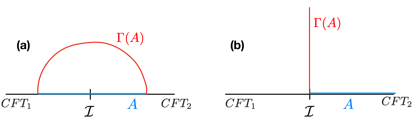
There are two qualitatively different choices for location of the interval in an interface CFT, as shown in figure 2. First, the interval can be chosen symmetrically around the defect [26, 27]. The minimal surface for such a symmetric interval is particularly simple in the AdS\AdS-sliced coordinates (3.34), and is given by z=z0z=z_{0} and u∈(−∞,∞)u\in(-\infty,\infty). The regularized length is given by

Length⁡(ΓA)=∫du=u∞−u−∞\displaystyle{\rm Length}(\Gamma_{A})=\int\differential{u}=u_{\infty}-u_{-\infty} (3.41)

We can use (3.37) to relate the FG cutoff ρ=ε\rho=\varepsilon, which furnishes the UV cutoff on the CFT side, to the cutoff u±∞u_{\pm\infty} in the AdS\AdS-sliced metric,

u±∞=±(−log⁡ε+log⁡(2​z0)+log⁡(cosh⁡q))\displaystyle u_{\pm\infty}=\pm\quantity\big(- \log\epsilon+ \log(2 z_0) +\log(\cosh q) ) (3.42)

Putting this together and using the expression for the central charge in terms of GN(3)G_{N}^{(3)} gives

SEE=c3​log⁡(2​z0ε)+c3​log⁡(cosh⁡q)\displaystyle S_{\rm EE}={c\over 3}\log{2z_0\over\epsilon}+{c\over 3}\log(\cosh q) (3.43)

Refer to caption

Figure 2: (a) The entagling surface AA is symmetric around the interface ℐ{\cal I}, (b) The entagleing surface AA is ends at the interface ℐ{\cal I}

Note that the first logarithmically divergent term is the standard expression for the entanglement entropy for a CFT without an interface present [28], since 2​z02z_{0} is the length of the interval. The constant term is universal in the presence of an interface and can be interpreted as the defect entropy (sometimes called g-factor [29]) associated with the interface.

Second, we can consider an interval which lies on one side of the interface and borders the interface [30, 31]. As shown in [32], the entangling surface is located at u=0u=0 and the entanglement entropy for an interval of length ll bordering the interface is given by

SEE′=c6​sech⁡(q)​log⁡(lε)\displaystyle S^{\prime}_{\rm EE}={c\over 6}\sech{q}\log{l \over\epsilon} (3.44)

3.4 All scalars

For completeness, we also present the general solution with all ϕI\phi_{I} scalars turned on. Let us define

αi​(u)\displaystyle\alpha_{i}(u) ≡ϕi​sinh⁡ΦΦ\displaystyle\equiv\frac{\phi_{i}\sinh\Phi}{\Phi} i\displaystyle i =1,2,3,4\displaystyle=1,2,3,4
βı¯​(u)\displaystyle\beta_{\bar{\imath}}(u) ≡ϕı¯​sinh⁡ΦΦ\displaystyle\equiv\frac{\phi_{\bar{\imath}}\sinh\Phi}{\Phi} ı¯\displaystyle\bar{\imath} =5,6,7,8\displaystyle=5,6,7,8 (3.45)

As a consequence of Eq. (3.12), the ratio ϕi′/ϕi\phi_{i}^{\prime}/\phi_{i} is the same for all ii so all the ϕi\phi_{i} scalars are proportional to each other. In other words, we have αi=ni​α\alpha_{i}=n_{i}\alpha for constants nin_{i} satisfying ni​ni=1n_{i}n_{i}=1, where α\alpha is given in Eq. (3.23). Then Eq. (3.15) becomes

α′2+βı¯′​βı¯′−(α′​α+βı¯′​βı¯)21+α2+βı¯​βı¯=α2\displaystyle\alpha^{\prime 2}+\beta_{\bar{\imath}}^{\prime}\beta_{\bar{\imath}}^{\prime}-\frac{(\alpha^{\prime}\alpha+\beta_{\bar{\imath}}^{\prime}\beta_{\bar{\imath}})^{2}}{1+\alpha^{2}+\beta_{\bar{\imath}}\beta_{\bar{\imath}}}=\alpha^{2} (3.46)

We can note that there exists a family of solutions where all βı¯\beta_{\bar{\imath}} functions satisfy

βı¯=nı¯​β\displaystyle\beta_{\bar{\imath}}=n_{\bar{\imath}}\beta (3.47)

for some function β\beta and constants nı¯n_{\bar{\imath}} satisfying nı¯​nı¯=1n_{\bar{\imath}}n_{\bar{\imath}}=1. When this is the case, Eq. (3.46) then further simplifies to

α′2+β′2−(α′​α+β′​β)21+α2+β2=α2\displaystyle\alpha^{\prime 2}+\beta^{\prime 2}-\frac{(\alpha^{\prime}\alpha+\beta^{\prime}\beta)^{2}}{1+\alpha^{2}+\beta^{2}}=\alpha^{2} (3.48)

which has already been solved in the previous section. We can prove that these are the only solutions to Eq. (3.46) which satisfy the equations of motion. The scalar dependence of the Lagrangian is

e−1​ℒ\displaystyle e^{-1}\mathcal{L} ⊃−g24​𝒫uI​𝒫uI+W\displaystyle\supset-\frac{g^{2}}{4}\mathcal{P}^{I}_{u}\mathcal{P}^{I}_{u}+W
=−g24​(α′2+βı¯′​βı¯′−(α′​α+βı¯′​βı¯)21+α2+βı¯​βı¯−(α2+2))\displaystyle=-\frac{g^{2}}{4}\quantity(\alpha'^2 + \beta_{\bi}' \beta_{\bi}' - \frac{(\alpha' \alpha+ \beta_{\bi}' \beta_{\bi})^2}{1 + \alpha^2 + \beta_{\bi} \beta_{\bi} } - (\alpha^2 + 2) ) (3.49)
If we write the βı¯\beta_{\bar{\imath}} in spherical coordinates, where we call the radius β\beta, this becomes
=−g24​(α′2+β′2+β2​K2−(α′​α+β′​β)21+α2+β2−(α2+2))\displaystyle=-\frac{g^{2}}{4}\quantity(\alpha'^2 + \beta'^2 + \beta^2 K^2 - \frac{(\alpha' \alpha+ \beta' \beta)^2}{1 + \alpha^2 + \beta^2 } - (\alpha^2 + 2) ) (3.50)

where K2K^{2} is the kinetic energy of the angular coordinates.22 2 Explicitly, let K2=θ′2+sin2​θ​ϕ′2+sin2​θ​sin2​ϕ​ψ′2K^{2}=\theta^{\prime 2}+\sin^{2}\theta\,\phi^{\prime 2}+\sin^{2}\theta\sin^{2}\phi\,\psi^{\prime 2}. We can treat α,β\alpha,\beta, and the three angles as the coordinates of this Lagrangian. The equation of motion from varying the Lagrangian with respect to α\alpha will only involve α\alpha and β\beta and their derivatives. Plugging-in (3.23) for α\alpha, satisfying this equation of motion fixes the form of β\beta to be what was found previously in Eq. (3.31). This means that Eq. (3.46) simplifies to β2​K2=0\beta^{2}K^{2}=0 and the three angles must be constant.

Therefore, the general solution is

ϕ​sinh⁡ΦΦ\displaystyle\frac{\phi\sinh\Phi}{\Phi} =|sinh⁡q|​sech⁡u\displaystyle=|\sinh q|\sech u
β\displaystyle\beta =sinh⁡p​cosh​q+cosh⁡p​sinh​q​tanh​u\displaystyle=\sinh p\cosh q+\cosh p\sinh q\tanh u
ϕi\displaystyle\phi_{i} =ni​ϕ,ni​ni=1\displaystyle=n_{i}\phi\qquad,\quad n_{i}n_{i}=1
ϕı¯​sinh⁡ΦΦ\displaystyle\frac{\phi_{\bar{\imath}}\sinh\Phi}{\Phi} =nı¯​β,nı¯​nı¯=1\displaystyle=n_{\bar{\imath}}\beta\qquad,\quad n_{\bar{\imath}}n_{\bar{\imath}}=1 (3.51)

4 Discussion

In this paper, we have presented Janus solutions for d=3d=3, 𝒩=8{\cal N}=8 gauged supergravity. We constructed the simplest solutions with the smallest number of scalars, namely the SO⁡(n,1)/SO⁡(8)\SO(n,1)/\SO(8) coset. The solutions we found have only two scalars displaying a nontrivial profile. One scalar is dual to a marginal operator O2O_{2} with scaling dimension Δ=2\Delta=2 and the other scalar is dual to a relevant operator O1O_{1} with scaling dimension Δ=1\Delta=1. We used the holographic correspondence to find the dual CFT interpretation of these solutions. It is given by a superconformal interface, with a constant source of the operator O2O_{2} which jumps across the interface. For the operator O1O_{1}, the source vanishes but there is an expectation value which depends on the distance from the interface. It would be interesting to study whether half-BPS Janus interfaces which display these characteristics can be constructed in the two-dimensional 𝒩=(4,4)\mathcal{N}=(4,4) SCFTs.

We considered solutions for the SO⁡(n,1)/SO⁡(8)\SO(n,1)/\SO(8) coset, but these solutions can be trivially embedded into the SO⁡(8,n)/(SO⁡(8)×SO⁡(n))\SO(8,n)/\quantity\big(\SO(8) \times\SO(n)) cosets with n>1n>1. Constructing solutions with more scalars with nontrivial profiles is in principle possible, but the explicit expressions for the quantities involved in the BPS equations are becoming very complicated. We also believe that the n=1n=1 case already illustrates the important features of the more general n>1n>1 cosets. Another possible generalization is given by considering more general gaugings. One important example is given by replacing the embedding tensor (2.6) with

ΘI​J,K​L=εi​j​k​ℓ+α​εı¯​ȷ¯​k¯​ℓ¯\displaystyle\Theta_{IJ,KL}=\varepsilon_{ijk\ell}+\alpha\varepsilon_{\bar{\imath}\bar{\jmath}\bar{k}\bar{\ell}} (4.1)

This is a deformation produces an AdS3\AdS_{3} vacuum which is dual to a SCFT with a large D1​(2,1,α)×D1​(2,1,α)D^{1}(2,1;\alpha)\times D^{1}(2,1;\alpha) superconformal algebra. As discussed in [16], this gauging is believed to be a truncation type II supergravity compactified on AdS3×S3×S3×S1\AdS_{3}\times S^{3}\times S^{3}\times S^{1} [33, 34]. It should be straightforward to adapt the methods for finding solutions developed in the present paper to this case.

We calculated the holographic defect entropy for our solution. It would be interesting to investigate whether this quantity can be related to the Calabi diastasis function following [35, 36]. For this identification to work we would have to consider the case n=2n=2 for which the scalar coset is a Kähler manifold.

We leave these interesting questions for future work.

Acknowledgements

We would like to thank Matteo Vicino for collaboration at the initial stages of this work and Per Kraus for useful conversations. The work of M. G. was supported, in part, by the National Science Foundation under grant PHY-19-14412. K. C. and M. G. are grateful to the Mani L. Bhaumik Institute for Theoretical Physics for support.

Appendix A Technical details

In this appendix, we present various technical details which are used in the main part of the paper.

A.1 SO⁡(8)\SO(8) Gamma matrices

We are working with 8×88\times 8 Gamma matrices ΓA​A˙I\Gamma^{I}_{A\dot{A}} and their transposes ΓA˙​AI\Gamma^{I}_{\dot{A}A}, which satisfy the Clifford algebra,

ΓA​A˙I​ΓA˙​BJ+ΓA​A˙J​ΓA˙​BI=2​δI​J​δA​B\displaystyle\Gamma^{I}_{A\dot{A}}\Gamma^{J}_{\dot{A}B}+\Gamma^{J}_{A\dot{A}}\Gamma^{I}_{\dot{A}B}=2\delta^{IJ}\delta_{AB} (A.1)

Explicitly, we use the basis in [37],

ΓA​A˙8\displaystyle\Gamma^{8}_{A\dot{A}} =1⊗1⊗1\displaystyle=1\otimes 1\otimes 1 ΓA​A˙1\displaystyle\Gamma^{1}_{A\dot{A}} =i​σ2⊗i​σ2⊗i​σ2\displaystyle=i\sigma_{2}\otimes i\sigma_{2}\otimes i\sigma_{2}
ΓA​A˙2\displaystyle\Gamma^{2}_{A\dot{A}} =1⊗σ1⊗i​σ2\displaystyle=1\otimes\sigma_{1}\otimes i\sigma_{2} ΓA​A˙3\displaystyle\Gamma^{3}_{A\dot{A}} =1⊗σ3⊗i​σ2\displaystyle=1\otimes\sigma_{3}\otimes i\sigma_{2}
ΓA​A˙4\displaystyle\Gamma^{4}_{A\dot{A}} =σ1⊗i​σ2⊗1\displaystyle=\sigma_{1}\otimes i\sigma_{2}\otimes 1 ΓA​A˙5\displaystyle\Gamma^{5}_{A\dot{A}} =σ3⊗i​σ2⊗1\displaystyle=\sigma_{3}\otimes i\sigma_{2}\otimes 1
ΓA​A˙6\displaystyle\Gamma^{6}_{A\dot{A}} =i​σ2⊗1⊗σ1\displaystyle=i\sigma_{2}\otimes 1\otimes\sigma_{1} ΓA​A˙7\displaystyle\Gamma^{7}_{A\dot{A}} =i​σ2⊗1⊗σ3\displaystyle=i\sigma_{2}\otimes 1\otimes\sigma_{3} (A.2)

The matrices ΓA​BI​J\Gamma^{IJ}_{AB}, ΓA˙​B˙I​J\Gamma^{IJ}_{\dot{A}\dot{B}} and similar are defined as unit-weight antisymmetrized products of Gamma matrices with the appropriate indices contracted. For instance,

ΓA​BI​J≡12​(ΓA​A˙I​ΓA˙​BJ−ΓA​A˙J​ΓA˙​BI)\displaystyle\Gamma^{IJ}_{AB}\equiv\frac{1}{2}(\Gamma^{I}_{A\dot{A}}\Gamma^{J}_{\dot{A}B}-\Gamma^{J}_{A\dot{A}}\Gamma^{I}_{\dot{A}B}) (A.3)

A.2 Integrability conditions

For BPS equations of the form

∂tε\displaystyle\partial_{t}\varepsilon =−12​z​γ0​(γ1+f⁡(u)+g⁡(u)​γ2)​ε\displaystyle=-\frac{1}{2z}\gamma_{0}\quantity\big( \gamma_1 + f(u) + g(u) \gamma_2)\varepsilon
∂zε\displaystyle\partial_{z}\varepsilon =−12​z​γ1​(f⁡(u)+g⁡(u)​γ2)​ε\displaystyle=-\frac{1}{2z}\gamma_{1}\quantity\big( f(u) + g(u) \gamma_2)\varepsilon
∂uε\displaystyle\partial_{u}\varepsilon =(F⁡(u)+G⁡(u)​γ2)​ε\displaystyle=\quantity\big(F(u) + G(u) \gamma_2)\varepsilon

where f,g,F,Gf,g,F,G are matrices acting on ε\varepsilon that commute with γa\gamma_{a}, the integrability conditions are

t,z:0\displaystyle t,z:\qquad 0 =(1+f2+g2)​ε+[f,g]​γ2​ε\displaystyle=(1+f^{2}+g^{2})\varepsilon+[f,g]\gamma_{2}\varepsilon
t,u:0\displaystyle t,u:\qquad 0 =(f′+[f,F]−{g,G})​ε+(g′+[g,F]+{f,G})​γ2​ε\displaystyle=(f^{\prime}+[f,F]-\{g,G\})\varepsilon+(g^{\prime}+[g,F]+\{f,G\})\gamma_{2}\varepsilon
z,u:\displaystyle z,u:\qquad\phantom{0} same as for ​t,u\displaystyle\qquad\text{same as for }t,u

A.3 Scalar asymptotics

The asymptotic expansions of the ϕ4\phi_{4} and ϕ5\phi_{5} scalar fields, as given in (3.32), in the limits u→±∞u\to\pm\infty are

|ϕ4|=\displaystyle|\phi_{4}|=  2​|sinh⁡q|​p±qsinh⁡(p±q)​e∓u\displaystyle\;2|\sinh q|\frac{p\pm q}{\sinh(p \pm q)}e^{\mp u}
−2​|sinh⁡q|sinh2⁡(p±q)​(p±qsinh⁡(p±q)​(sinh2​p+sinh2​q)±2​sinh​p​sinh​q)​e∓3​u+𝒪⁡(e∓5​u)\displaystyle-\frac{2|\sinh q|}{\sinh^{2}(p\pm q)}\quantity( \frac{p \pm q}{\sinh(p \pm q)} (\sinh^2 p + \sinh^2 q) \pm 2 \sinh p \sinh q )e^{\mp 3u}+\mathcal{O}(e^{\mp 5u})
ϕ5=\displaystyle\phi_{5}= (p±q)−2sinh⁡(p±q)​(p±qsinh⁡(p±q)​sinh2​q±sinh⁡p​sinh⁡q)​e∓2​u+𝒪⁡(e∓4​u)\displaystyle\;(p\pm q)-\frac{2}{\sinh(p \pm q)}\quantity( \frac{p \pm q}{\sinh(p \pm q)} \sinh^2 q \pm\sinh p \sinh q )e^{\mp 2u}+\mathcal{O}(e^{\mp 4u}) (A.4)

References