State Predictive Information Bottleneck
Abstract
The ability to make sense of the massive amounts of high-dimensional data generated from molecular dynamics (MD) simulations is heavily dependent on the knowledge of a low dimensional manifold (parameterized by a reaction coordinate or RC) that typically distinguishes between relevant metastable states and which captures the relevant slow dynamics of interest. Methods based on machine learning and artificial intelligence have been proposed over the years to deal with learning such low-dimensional manifolds, but they are often criticized for a disconnect from more traditional and physically interpretable approaches. To deal with such concerns, in this work, we propose a deep learning based State Predictive Information Bottleneck (SPIB) approach to learn the RC from high dimensional molecular simulation trajectories. We demonstrate analytically and numerically how the RC learnt in this approach is deeply connected to the committor in chemical physics, and can be used to accurately identify transition states. A crucial hyperparameter in this approach is the time-delay, or how far into the future the algorithm should make predictions about. Through careful comparisons for benchmark systems, we demonstrate that this hyperparameter choice gives useful control over how coarse-grained we want the metastable state classification of the system to be. We thus believe that this work represents a step forward in systematic application of deep learning based ideas to molecular simulations in a way that bridges the gap between artificial intelligence and traditional chemical physics.
I Introduction
Rapid advances in computational power have made molecular dynamics (MD) a powerful tool for studying systems in biophysics, chemical physics and beyond. However, there are still at least two open questions in this area: first, how to make use of the deluge of data generated from MD simulation understandable for a human; second, how to further extend timescales that can be reached in MD. The unifying aspect to overcoming both these difficulties is to efficiently uncover a low dimensional manifold (parameterized by a reaction coordinate or RC) on which the dynamics of the system can be projected.Wang, Lamim Ribeiro, and Tiwary 2020
Over the past decades, various approaches have been developed to learn the RC from trajectory data. It has been argued that for given two states, the committor, defined next, is a perfect candidate for the RC as it provides a quantitative description of the dynamics along a trajectory.Bolhuis, Dellago, and Chandler 2000; Bolhuis et al. 2002 Let A and B denote the reactant and product states, then the committor probability is defined as the probability of the trajectories that reach state B prior to the state A from a conformation . Through the analysis of the committor distribution, much insight has been obtained in a variety of phenomena ranging from ion solvation to biomolecular isomerization,Bolhuis, Dellago, and Chandler 2000; Geissler, Dellago, and Chandler 1999; Pluharova et al. 2016; Roy et al. 2016 Transition path sampling (TPS), which focuses on sampling the pathways connecting metastable states, is a powerful tool to analyze the committor.Dellago et al. 1998; Bolhuis et al. 2002; Best and Hummer 2005a Based on it, some physically meaningful RC can then be identified through a generic algorithmMa and Dinner 2005 or a likelihood maximization approachPeters and Trout 2006; Peters 2016. However, these methods always heavily depend on human intuition to generate the trial coordinates.Peters 2016
Another approach to obtaining the RC is to learn the relevant slow modes of dynamics. Coifman, Kevrekidis, Clementi and others first used diffusion map to determine collective reaction coordinates for macromolecular dynamics.Nadler et al. 2006; Coifman et al. 2008; Rohrdanz et al. 2011 Thereafter, Noé and coworkers proposed the variational approach to conformation dynamics (VAC) and combined it with the time-lagged independent component analysis (TICA) to identify the optimal “slow subspace” from a large set of prior order parameters.Noé and Nuske 2013; Pérez-Hernández et al. 2013 More recently a generalized version called VAMPnets was developed by the same group leveraging the power of neural networks.Mardt et al. 2018 In a similar spirit, the SGOOP method by Tiwary and Berne used an iterative approach to find RC through a maximum path entropy framework.Tiwary and Berne 2016 Though all these slow-mode based methods are highly interpretable, the optimization can usually be difficult unless some simplifications are made. For instance, in TICA and SGOOP these simplifications could include learning the RC as linear combinations of pre-selected order parameters.Pérez-Hernández et al. 2013; Tiwary and Berne 2016
Besides these two physics-based approaches, other statistical approaches have also been developed to learn RC through a more flexible framework, such as VDEHernandez et al. 2018 and RAVERibeiro et al. 2018; Wang, Ribeiro, and Tiwary 2019. In the RAVE approach for instance, the RC is interpreted as a bottleneck or a low dimensional space that predicts the most important features of the simulated trajectories. Such a RC can then be learned by making a trade-off between prediction and model complexity through an objective function. Typically a variational Bayesian approach is employed to allow these methods to parameterize the objective function using a neural network and achieve highly efficient training.Kingma and Welling 2013; Alemi et al. 2016 Arguably these methods can be less expensive than physics-based approaches, but they may also be uninterpretable and therefore unreliable since the relationship between the statistics-based RC and the traditional physics-based RC is still unclear.
In this work, we develop a State Predictive Information Bottleneck (SPIB) framework that allows us to efficiently and accurately learn a RC from MD trajectories. Most importantly, we demonstrate rigorously how the slow bottleneck variable learnt in RAVE and related deep learning based methods can qualify as a good RC with the same attributes as expected from the committor. Similar to RAVERibeiro et al. 2018; Wang, Ribeiro, and Tiwary 2019, we also assume that RC should carry only the minimal information of the past to still be able to reliably predict the future state of the system. The key feature that makes SPIB stand out is that a discrete-state representation of this system is learned on-the-fly during the training process and guides our RC to focus only on the motion related to the state-to-state transitions. We show analytically and numerically that the RC learned by our algorithm is related to the committor, and demonstrate that it can capture the important information from the trajectory to identify the correct transition state. Moreover, we demonstrate how our algorithm can automatically figure out the metastable states in a complex system and generate an accurate but still highly understandable description of their inter-conversion dynamics. Given these promising properties, we believe our algorithm can be a powerful tool to analyze generic complex systems.
II Method
II.1 Information Bottleneck
The Information Bottleneck (IB) principle provides a general framework to learn a concise representation of an input source that is maximally informative about some target .Tishby, Pereira, and Bialek 2000; Alemi et al. 2016 Here typically the representation has much smaller dimensionality than the source , while the target can be of low or high dimensionality depending on the task at hand. The IB principle postulates that the desired representation should use minimal information from the input to predict the target . Mathematically, such a learning process can be formulated as maximizing the objective function:
| (1) |
Here, the function denotes the mutual information between any two random variables. The trade-off between the prediction capacity and model complexity is controlled by the Lagrange multiplier . Unfortunately, the direct optimization of the information bottleneck shown in Eq. 1 is impractical as the calculation of mutual information in general is computationally expensive. Alemi et al. 2016; Wang, Ribeiro, and Tiwary 2019 Thus, following Ref. Alemi et al. 2016, we can obtain a variational lower bound on the original objective function from Eq. 1:
| (2) | ||||
where and are variational approximations to the true probability distributions and respectively. Notice that the entropy of the targets in Eq. 2 is independent of the optimization process and hence can be ignored. From a coding theory perspective,Berlekamp 2015 as can be interpreted as a latent representation or a code, we usually refer to as a probabilistic encoder, and as a probabilistic decoder. Interestingly, one can easily obtain from Eq. 2 the objective function used in variational autoencoders by assuming and requiring the representation to reconstruct the input instead of predicting a target .Kingma and Welling 2013; Alemi et al. 2016 Based on rate-distortion theory,Shannon 1959; Alemi et al. 2018 the first term in Eq. 2 can be interpreted as the distortion, which measures the ability of our representation to predict the desired target, while the second term can be interpreted as the rate, which measures the number of bits per data sample to be transmitted. Thus, maximizing can also be viewed as the problem of determining the minimal number of bits, as measured by the rate, that should be communicated from a source through a channel so that the receiver can reconstruct the original signal without exceeding a desired value of the distortion.
There are many possible choices for the encoder , the decoder and the approximate prior , depending on the particular application domain. We point out here that all these three probability distributions can depend collectively on some model parameters , which are learned during the training process. Therefore, in the following sections, we will add a subscript to all these three distributions .
II.2 State Predictive Information Bottleneck
The generic IB framework introduced in Sec. II.1 leaves ample scope for the specific flavor of implementation in many different ways, as for instance we demonstrated in our past publications through the RAVE family of methods,Ribeiro et al. 2018; Wang, Ribeiro, and Tiwary 2019 and it has been discussed more generally in Ref. Alemi and Fischer 2018. Based on the general IB framework, in this section we advance our RAVE family of methods with a State Predictive Information Bottleneck (SPIB) framework. Similar to existing RAVE formulations here as well we aim to learn an accurate reaction coordinate (RC) for generic molecular systems, but make RAVE significantly more robust in many aspects, and draw rigorous and useful connections between the past-future information bottleneck and the committor based definition of the RC in theoretical chemistry.Bolhuis, Dellago, and Chandler 2000; Best and Hummer 2005b However unlike RAVE, where the aim is to predict a time-delayed version of the entire input molecular configuration, here we set as target in Eq. 1 its future state, which is drawn from a dictionary of indices for possible metastable states. The target is relatively much lower in dimensionality than the exact molecular configuration. In this way, we require our RC to only predict which state the system will stay in after a time delay , instead of its exact configuration. Typically the number and location of such states are not available a priori and our work makes it possible to estimate these robustly and on-the-fly, as we demonstrate in Sec. II.4.
The main advantage of such a simplification of the prediction task is that only the motion related to the transitions between different states will be captured by the learnt RC, while the fluctuations inside any metastable state will be ignored. Thus, for a given unbiased trajectory and its corresponding state labels with large enough , the objective function of SPIB can be formulated as:
| (3) | ||||
where is sampled from and the time interval between and is the time delay .
In SPIB, the trajectory is usually expressed in terms of many order parameters or features, while the state labels are mutually exclusive and expressed in terms of one-hot vectors, i.e. a binary vector with a single high (1) bit and all the others low (0). To implement this we use a deep feed forward neural network with softmax outputs in our decoder .
| (4) |
where the state label is a one-hot vector of dimensions and the decoder function is the -dimensional softmax output of a neural network.
Given that we expect the learnt RC should demarcate between different metastable states, it is natural to assume a multi-modal distribution for the prior . In our algorithm, we employ the variational mixture of posteriors prior (VampPrior) to obtain such a multi-modal prior distribution.Tomczak and Welling 2017 Here, the approximate prior is a weighted mixture of different posteriors with pseudo-inputs in lieu of :
| (5) |
where is the number of pseudo-inputs, is a vector which has the same dimension as input , and represents the weight of under the constraint . The pseudo-inputs and weights can be thought of the parameters of the prior, which are learned through backpropagation of the objective function (Eq. 3). In principle, the number of pseudo-inputs should be equal to the number of metastable states in the system. In practical settings however for real-world applications to complex molecular systems, the number of metastable states is unknown a priori. To deal with such cases, the simple and powerful solution is to choose a large enough making the prior more flexible.
Finally, for simplicity, we take the encoder in Eq. 5 as a neural network with a multivariate Gaussian output:
| (6) |
where the mean and variance are outputs of a neural network whose input is . is the identity matrix. Then we can use the reparameterization trickKingma and Welling 2013 to write and , where and the encoder function is a deterministic nonlinear function parameterized by a neural network.
II.3 Dependence of SPIB on
In RAVEWang, Ribeiro, and Tiwary 2019 as well as in this algorithm, the time delay plays an important role in the simplification of the learning process. A time delay is tantamount to ignoring the dynamics completely and simply clustering the input configuration into different states, while can filter out all the fast modes, helping us ignore unnecessary details of the dynamical processes. Given its critical importance, in this section we analyze in detail.
Given a Markov process , if the initial probability distribution is given by , the corresponding probability distribution after a lag time is
| (7) |
where the time evolution of the probability density is governed by a linear operator , called the propagator for the process . To explain the role of the time delay in our algorithm, we can derive a spectral decomposition for this operator by assuming the dynamics is reversible:Berezansky, Sheftel, and Us 1996
| (8) |
where are the propagator’s eigenfunctions and are the eigenvalues which decay exponentially in time with rates . In principle, SPIB will ignore the dynamical processes whose timescale is comparable to or even smaller than the time delay , as its corresponding component in Eq. 8 will decay exponentially. Thus, we interpret the time delay as the minimal time resolution that we seek to maintain for the dynamical system.
As discussed in the previous subsection, SPIB predicts from the present configuration the future state instead of the exact configuration . A subtle assumption made to justify this simplification is that the fluctuation inside each metastable state should be much faster than the transitions between different states. Such a timescale separation allows us to rewrite Eq. 8 as a sum of the stationary state eigenvector and two other parts:
| (9) | ||||
The first slow processes correspond to the state-to-state transitions that we are interested in, while the fast processes represent the motions related to the molecular relaxation within these states. Therefore, an appropriate time delay should satisfy in order to screen out all the fast processes. In practice, this can be checked by examining the robustness of the results against different values of , as we show in Sec. III.
II.4 Discrete-State Representation and Iterative Retraining Algorithm
The SPIB framework introduced thus far requires a prior knowledge of states in the system, which is usually intractable especially for complex systems. To surmount this limitation, here we introduce an iterative technique to obtain a converged discrete-state representation based on the selected time delay we described in Sec. II.3. The central idea is that if one configuration was located at state at a certain time, then after time delay , it should still have the largest probability to be found at state , since is much shorter than the typical escape time from a metastable state.
Given a set of initial state labels , we can write down the optimal predictor by assuming ergodic dynamics and setting it equal to a vector of probabilities :
| (10) | ||||
Here is the state label function that maps the trajectory to the -dimensional state labels , and represents the equilibrium density of . can be interpreted as the probability that the system starting from will be found in state after a time delay . As it is a function of the input configuration and represents a state-transition probability, we call the function as the state-transition density.
With this set-up, we now introduce a simple iterative scheme that is at the heart of our SPIB approach, as it allows us to learn the number and location of states on the fly with minimal human intervention. We start with an arbitrary set of labels for the system, where both the number and location of labels are some initial guess. If the system initiated from a certain high-dimensional configuration has the largest probability to be found after time delay in some state from these initial labels, then the label of the configuration will be refined and updated to state . We can denote the deterministic output of SPIB as , which tries to approximate the best predictor . Then a set of new state labels can be generated by:
| (11) |
This label refinement step might very well lead to null assignments for some of the labels we started with, as shown in Sec. III for actual test cases.
Based on Eq. 10 and 11, an iterative retraining can be performed and the whole algorithm is summarized through Fig. 1(b) and Alg. 1. Thus, as illustrated above, we expect such a converged discrete-state representation , by this self-consistent design, should only depend on the dynamic properties of the system and the time delay . Moreover, on account of the screening property of the time delay , the final representation will automatically ignore transient intermediate states and only figure out those long-lived metastable states. This in fact offers us a powerful tool to obtain a dynamics-based coarse-grained description of the complex system.

II.5 State-Transition Density and Committor
Recently a few methods have been proposed to calculate the committor through the construction of Markov state models (MSM).Swope, Pitera, and Suits 2004; Noé and Fischer 2008; Wales 2009; Lane et al. 2011; Thiede et al. 2019 By constructing an efficient MSM, the committor can be calculated directly from the transition matrix by solving a system of linear equations.Noé and Fischer 2008 However, this usually requires a large number of discrete states in order to estimate the MSM transition matrix and thus the committor accurately Wales 2009; Lane et al. 2011; Thiede et al. 2019, thereby severely diminishing the interpretability of the model. This also means requiring a very well sampled trajectory moving accurately capturing transitions between the large number of different states, which might be hard to achieve.Biswas, Lickert, and Stock 2018 As we will show in this section, our SPIB approach can efficiently estimate the transition density by relegating the need to know the exact transition probabilities within the metastable states of the system. In other words, we will demonstrate that SPIB can learn the approximate committor and identify correct transition state regions even with a small number of discrete states relative to MSM type approaches.
As discussed in the Sec. II.3, the timescale separation between the state-to-state transitions and the fluctuations inside each metastable state allows the factorization of the transition density into two parts:
| (12) | |||
In Eq. 12, the first part represents the equilibrium probability density for any state , while the second part is exactly the state-transition density defined in Eq. 10. Given the definition of two states A and B whose committor attracts our interest, the committor then can be obtained by solving following linear integral equations:
| (13) | |||||
However, instead of solving Eq. 13 explicitly and tabulating configurations where , the transition state ensemble (TSE) can also be identified using this state-transition density directly. If a set of trajectories starting from some have the largest, approximately equal probabilities of transitioning to two different states after time delay , then can be considered to belong to the TSE. Through the numerical examples in the section III, we will illustrate that this new definition of transition states is, in fact, as valid as the original committor-based definition. Besides, we would also like to highlight that based on this definition and Alg. 1, the ensemble of transition states will eventually form the boundaries of the finally converged discrete states. Therefore, the state-transition density provides us with an accurate but intuitive way to characterize the transitions between different metastable states.
Overall, we believe that such a state-transition density finally generated by our algorithm is a reasonable substitute for the committor as it can quantitatively describe the dynamical behaviors of every states along a trajectory and further identify the correct transition states. Thus, the most informative representation given by the encoder about this state-transition density learned by SPIB should naturally serve as a reasonable RC approximating the committor. But for simplicity, in the following discussion, our RC will refer specifically to the deterministic part or the mean value of the representation to better compare with traditional deterministic prescriptions.
III Results
III.1 Model Systems
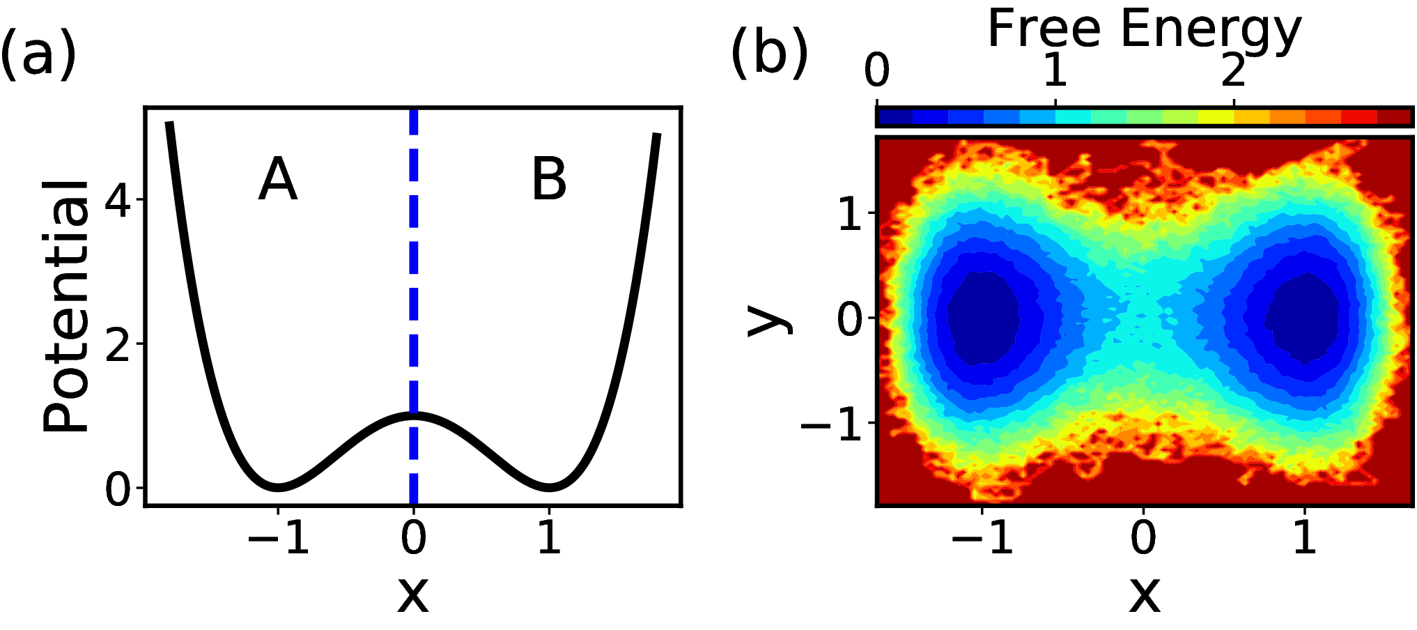
To demonstrate our SPIB approach in practice, here we benchmark it for different model potentials, including two analytical potentials, and the small biomolecule alanine dipeptide in vacuum. The first analytical potential comprises a double well in two dimensions, shown in Fig. 2. The second potential is made of four wells also in two dimensions, shown in Fig. 5. The governing potentials are given by
| (14) |
and
| (15) | ||||
The trajectories for these two potentials were generated using Langevin dynamics simulationBussi and Parrinello 2007 with integration timestep of 0.001 units, inverse temperature and friction coefficient , where is Boltzmann constant. For either potential, we used a long equilibrium trajectory equaling 60,000 time units with a temporal resolution of 0.01 units.
For the study of conformation transitions in alanine dipeptide in vaccum, the simulation was performed with the software GROMACS 5.0,Berendsen, van der Spoel, and van Drunen 1995; Abraham et al. 2015 patched with PLUMED 2.4.Tribello et al. 2014 The temperature was kept constant at 450 K using the velocity rescaling thermostatBussi, Donadio, and Parrinello 2007 and the integration time step was 2 fs. A 800 ns long equilibrium trajectory with a temporal resolution of 0.01 ps was employed to train and test our algorithm.
III.2 Neural network architecture and training
In this paper, both the encoder and decoder are nonlinear and parameterized by fully connected neural networks with two hidden layers as shown in Fig. 1(a). Each hidden layer in both the encoder and decoder has 16 nodes for the two analytical potentials, and 64 nodes for alanine dipeptide. All these hidden layers use a rectified linear unit (ReLU) as the activation function.
The networks were trained using the Adam optimizerKingma and Ba 2014 with a learning rate of and a batch size of 2048 for all the numerical examples. The state labels are refined every 1000 training steps for analytical potentials, and every 2000 training steps for alanine dipepetide.
III.3 Double-Well Analytical Potential
We first demonstrate SPIB for the double-well analytical potential. For this first example, we assume we already know the system relatively well by setting the RC dimension , the number of pseudo-inputs and the dimension of state labels . In following sections III.4 and beyond, we remove the need for making any such assumptions and show how SPIB still works very well. For this double well system, in order to generate an initial guess of state labels, the samples are labeled as state A if and B otherwise. Here, the initial boundary point can be changed to test the robustness of SPIB.

The final converged results are shown in Fig. 3. Fig. 3(a) illustrates that SPIB can learn the correct state labels, where the boundary is located at around . In Fig. 3(b), as the -direction is pure noise, the learned RC is almost independent of the direction, suggesting that SPIB is able to distinguish important features from noise. Besides, Fig. 3(b) also shows that as desired, the fluctuations inside each state are not captured by SPIB, as they are almost mapped to a single point in RC. Fig. 3(c) and (d) present the state-transition density learned by our algorithm, which is highly correlated with our RC.
We now further demonstrate that our results obtained above are robust to the initial boundary demarcating parameter and the time delay . As shown in Fig. 4, a large range of and values can result in the same state definition. The fractional population of state A is defined by the ratio of the number of samples finally labeled as state A to the total number of samples (). For the initial boundary point , the only constraint is that it should not be large than 1 or smaller than -1; otherwise, state A and state B will be regarded as one state by our algorithm. can be anywhere between the molecular relaxation time scale () and the interconversion timescale between state A and B, which is around the implied timescale of shown in Supplementary Material (SM).
Here, all the results are obtained by setting the hyper-parameter in Eq. 3 (not to be confused with the inverse temperature ), which can be determined by choosing the turning point on the Rate-Distortion plot (see SM). However, as long as is not too large, we found our results are still very robust to the selection of .

III.4 Four-Well Analytical Potential
We now apply SPIB to a four-well analytical potential where we do not assume any prior knowledge about the system such as the number of metastable states. In this case, we arbitrarily discretized the input data space into sufficiently fine grids as our initial state labels, shown in Fig. 6(a). We set the RC dimension , the number of pseudo-inputs and the dimension of state labels . In other words, here we have deliberately taken and to be arbitrarily large relative to the true number of metastable states. In order to let the RC only contain the important information, we chose (see SM).
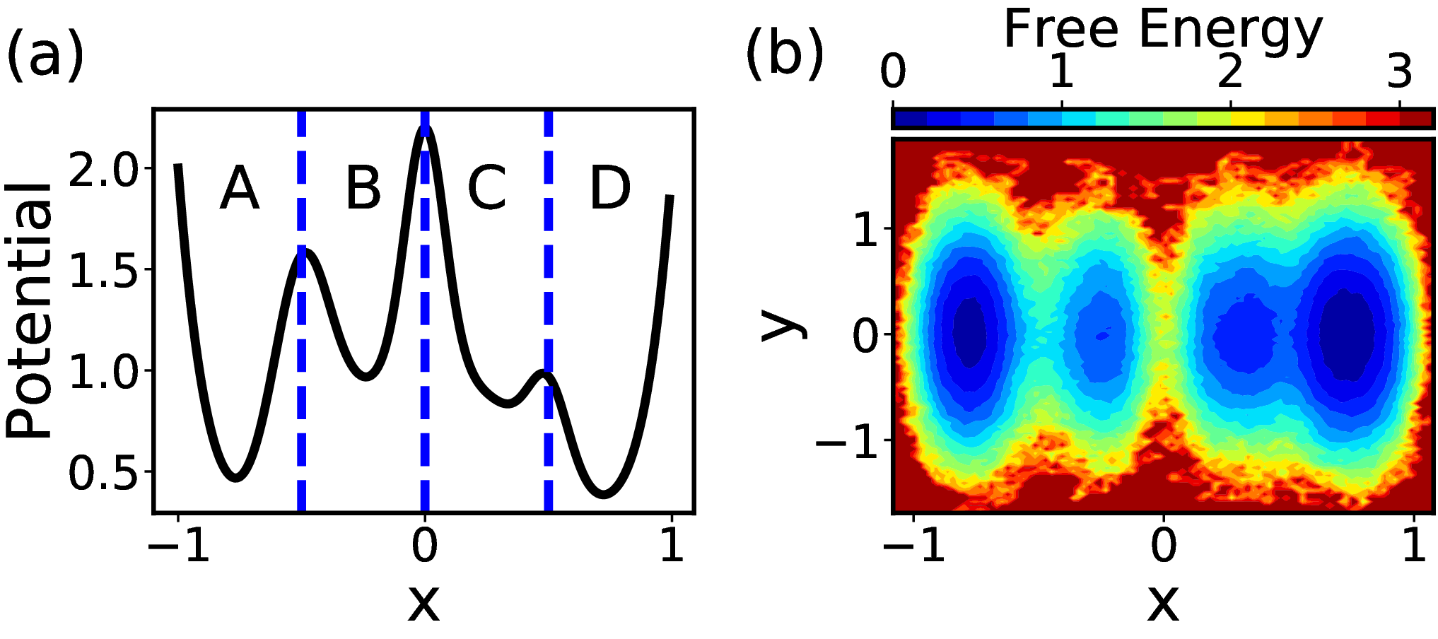


Fig. 6 shows the state labels and RC learned by SPIB using different time delays . There are several interesting observations that can be made here. Firstly, in Fig. 6(b), we find that SPIB can still obtain the correct state labels by choosing an appropriate time delay () without any prior information. This is very promising for practical problems as a precise state definition or even the number of states are usually unavailable in complex systems. Secondly, we also find that a dynamically truthful discrete-state representation can be obtained by SPIB using different time delays . When the time delay increases (), the original state C and state D shown in Fig. 5(a) cannot be distinguished by SPIB any more (Fig. 6(c)). If we further increase the time delay (), even the original state A and state B will become indistinguishable (Fig. 6(d)). The time dependence of state labels can be explained by the different timescales of transitions between states (Fig. 8). These results unequivocally shed light into the role of the time delay in our algorithm–it filters out the fast modes of dynamics, and provides a dynamics-based coarse-gained understanding of the complex system. We also point out that although our results depend on the selection of time delay, they are in fact still very robust to changes of . Fig. 7 shows a broad range of can result in the same discrete-state representation.
III.5 Alanine Dipeptide in Vacuum
Finally, we employ SPIB to study conformation transitions in the small biomolecule alanine dipeptide. The trajectory here was expressed in terms of four dihedral angles , , and , illustrated in Fig. 9. Here we discretized the input data space along into 10 grids as our initial state labels, as shown in Fig. 10(a), and set the RC dimension , the number of pseudo-inputs and the dimensionality of state labels . was chosen to generate the most informative RC.


Similar to our previous results for four-well analytical potential, in Fig. 10(b), we show how SPIB can still learn successfully the state labels corresponding to the three well-known free energy minima in the - space shown in Fig. 9(b). When the time delay = , the two free energy minima located in the top-left corner of the - space (Fig. 9(b)) become indistinguishable from a dynamical perspective, given that the interconversion times between these two metastable states is now close to (Fig. 12). Thus, only 2 states are obtained in Fig. 10(c). We then further demonstrate in Fig. 11 that such a coarse-grained understanding obtained by SPIB is still very robust in alanine dipeptide, as the same state labels are obtained with a broad range of .


The 2-D RC so learnt through SPIB is presented in Fig. 10(d-g). The free energy surface in the RC space shown in Fig. 10(f,g) indicates that the barrier between and defined in Fig. 9(b) is much higher than the barrier between the two local minima (state and state in Fig. 10(b,d)) within . This also explains why different interconversion timescales are obtained in Fig. 12. From these results, we can see that a 1-D RC is enough if we just want to identify the transitions between and . Thus, we reran the analysis of with the RC dimension and show the new RC so-obtained in Fig. 13(a). Such a 1D RC can be easily used to identify the transition state, which has the same state transition probability to two different metastable states. In Fig. 13(a), the transition state corresponds to . To test whether our RC can identify the correct transition states, we chose to focus on the states located in the TS region shown in Fig. 9(b). By doing a traditional, detailed committor analysis, we obtained the reference committor. For this we launched 50 1-ps trajectories with random initial Maxwell-Boltzmann velocities for each configuration in vicinity of the TS under the constraint , and then calculated their committor function based on the fraction of trajectories reaching prior to . This committor probability distribution is shown in Fig. 13(b), where it can be seen clearly that the probability of is characterized by a single peak centered at . This shows that the RC from SPIB indeed meets the traditional expectations from a RC.Best and Hummer 2005b

We now show in Fig. 13(c,d) our learned state-transition density to the state projected in the - plane and - plane. Fig. 13(c) shows that the transition states in TS region are aligned almost parallel to the axis, suggesting they are in fact almost irrelevant to . Fig. 13(d), however, indicates that both and are required in order to identify the transition state. Both of these findings are in good agreement with previous reports for this system.Bolhuis, Dellago, and Chandler 2000; Ma and Dinner 2005; Mori et al. 2020 Thus, our results confirm that the state-transition density generated by SPIB can be a reasonable substitute for the committor, and the RC learned can capture the most important dynamical information from the input trajectory to identify the correct transition states.
IV Discussion
In this work, we have proposed a deep learning based algorithm called State Predictive Information Bottleneck (SPIB) to learn the RC from trajectory data. SPIB builds up on the insights we have introduced previously in the RAVE family of methods,Ribeiro et al. 2018; Wang, Ribeiro, and Tiwary 2019 and by changing the nature of the information bottleneck based objective function, it allows generating new physical insights from typically hard to interpret deep neural networks. We have first showed that the time delay can be interpreted as the time resolution that we care about in a dynamical system, and through this we can control the degree of coarse-graining obtained by our algorithm. Once a time delay is selected, SPIB can automatically index the high-dimensional state space into metastable states through an iterative retraining algorithm, and then characterize their dynamic behaviors in terms of state-transition density. This provides us with a promising way to analyze generic complex systems and interpret the massive data generated by MD simulations.
We have also demonstrated that the bottleneck variable learned in SPIB tries to carry the maximum information of the state-transition density, which in principle can be equivalent to the traditional committor function, if there is a timescale separation between the state-to-state transitions and the fluctuations within metastable states. Then through numerical tests on benchmark systems, we confirmed that the state-transition density generated by SPIB is a reasonable substitute for committor, and demonstrated that our RC can focus only on the motion related to state transitions and capture the most important features from trajectories to identify the correct transition states.
We finish this section by describing some of the exciting new avenues pertaining to SPIB that we will explore in future work. First pertains to the use of SPIB for enhanced sampling. By choosing an appropriate time delay, the RC learned by SPIB can correctly identify different metastable states and even the transition states among them, which can be crucial to obtain better sampling.Bussi and Laio 2020 This would involve reweighting input biased trajectories, obtained by biasing along some trial RC for instance. The reweighting can then be performed in the manner described in Ref. Ribeiro et al. 2018; Wang, Ribeiro, and Tiwary 2019. Secondly, it is natural to desire that the RC learned by SPIB can be interpreted in terms of a few human-understandable physical variables. However, unlike RAVEWang, Ribeiro, and Tiwary 2019 here we use a nonlinear deep neural network as our encoder, and thus the interpretation of our RC is not a trivial task. In order to deal with this question of interpretability, we will make use of approaches in representation learning.Bengio, Courville, and Vincent 2013 Overall, we believe our algorithm is a step towards a more complete understanding of complex systems by making use of the variability offered by the information bottleneck framework of AI,Tishby, Pereira, and Bialek 2000; Alemi et al. 2016; Alemi and Fischer 2018 and should be useful to a broad range of scientific communities.
Supplementary material
See supplementary material for other numerical details.
Acknowledgements
This research was entirely supported by the U.S. Department of Energy, Office of Science, Basic Energy Sciences, CPIMS Program, under Award DE-SC0021009. The authors thank Sun-Ting Tsai for sharing the code implementing Langevin dynamics, Luke Evans for sharing the GROMACS script, Yihang Wang and Zachary Smith for in-depth discussions. The authors also thank MARCC and XSEDE for providing computational resources used in this work.
Code availability statement
The python code of SPIB using Pytorch will be made available for public use at https://github.com/tiwarylab/State-Predictive-Information-Bottleneck.
Data availability statement
The data that support the findings of this study are available from the corresponding author upon reasonable request.
References
References
- Wang, Lamim Ribeiro, and Tiwary (2020) Y. Wang, J. M. Lamim Ribeiro, and P. Tiwary, Curr Opin Struct Biol 61, 139 (2020).
- Bolhuis, Dellago, and Chandler (2000) P. G. Bolhuis, C. Dellago, and D. Chandler, Proc Natl Acad Sci U S A 97, 5877 (2000).
- Bolhuis et al. (2002) P. G. Bolhuis, D. Chandler, C. Dellago, and P. L. Geissler, Advances in chemical physics 53, 291 (2002).
- Geissler, Dellago, and Chandler (1999) P. L. Geissler, C. Dellago, and D. Chandler, The Journal of Physical Chemistry B 103, 3706 (1999).
- Pluharova et al. (2016) E. Pluharova, M. D. Baer, G. K. Schenter, P. Jungwirth, and C. J. Mundy, The Journal of Physical Chemistry B 120, 1749 (2016).
- Roy et al. (2016) S. Roy, M. D. Baer, C. J. Mundy, and G. K. Schenter, The Journal of Physical Chemistry C 120, 7597 (2016).
- Dellago et al. (1998) C. Dellago, P. G. Bolhuis, F. S. Csajka, and D. Chandler, The Journal of chemical physics 108, 1964 (1998).
- Best and Hummer (2005a) R. B. Best and G. Hummer, Proceedings of the National Academy of Sciences 102, 6732 (2005a).
- Ma and Dinner (2005) A. Ma and A. R. Dinner, The Journal of Physical Chemistry B 109, 6769 (2005).
- Peters and Trout (2006) B. Peters and B. L. Trout, The Journal of chemical physics 125, 054108 (2006).
- Peters (2016) B. Peters, Annual review of physical chemistry 67, 669 (2016).
- Nadler et al. (2006) B. Nadler, S. Lafon, R. R. Coifman, and I. G. Kevrekidis, Applied and Computational Harmonic Analysis 21, 113 (2006).
- Coifman et al. (2008) R. R. Coifman, I. G. Kevrekidis, S. Lafon, M. Maggioni, and B. Nadler, Multiscale Modeling & Simulation 7, 842 (2008).
- Rohrdanz et al. (2011) M. A. Rohrdanz, W. Zheng, M. Maggioni, and C. Clementi, The Journal of chemical physics 134, 03B624 (2011).
- Noé and Nuske (2013) F. Noé and F. Nuske, Multiscale Modeling & Simulation 11, 635 (2013).
- Pérez-Hernández et al. (2013) G. Pérez-Hernández, F. Paul, T. Giorgino, G. De Fabritiis, and F. Noé, The Journal of chemical physics 139, 07B604_1 (2013).
- Mardt et al. (2018) A. Mardt, L. Pasquali, H. Wu, and F. Noé, Nature communications 9, 1 (2018).
- Tiwary and Berne (2016) P. Tiwary and B. Berne, Proceedings of the National Academy of Sciences 113, 2839 (2016).
- Hernandez et al. (2018) C. X. Hernandez, H. K. Wayment-Steele, M. M. Sultan, B. E. Husic, and V. S. Pande, Phys Rev E 97, 062412 (2018).
- Ribeiro et al. (2018) J. M. L. Ribeiro, P. Bravo, Y. Wang, and P. Tiwary, The Journal of Chemical Physics 149, 072301 (2018).
- Wang, Ribeiro, and Tiwary (2019) Y. Wang, J. M. L. Ribeiro, and P. Tiwary, Nature communications 10, 3573 (2019).
- Kingma and Welling (2013) D. P. Kingma and M. Welling, arXiv preprint arXiv:1312.6114 (2013).
- Alemi et al. (2016) A. A. Alemi, I. Fischer, J. V. Dillon, and K. Murphy, arXiv preprint arXiv:1612.00410 (2016).
- Tishby, Pereira, and Bialek (2000) N. Tishby, F. C. Pereira, and W. Bialek, arXiv preprint physics/0004057 (2000).
- Berlekamp (2015) E. R. Berlekamp, Algebraic coding theory (revised edition) (World Scientific, 2015).
- Shannon (1959) C. E. Shannon, IRE Nat. Conv. Rec 4, 1 (1959).
- Alemi et al. (2018) A. Alemi, B. Poole, I. Fischer, J. Dillon, R. A. Saurus, and K. Murphy, (2018).
- Alemi and Fischer (2018) A. A. Alemi and I. Fischer, arXiv preprint arXiv:1807.04162 (2018).
- Best and Hummer (2005b) R. B. Best and G. Hummer, Proceedings of the National Academy of Sciences 102, 6732 (2005b).
- Tomczak and Welling (2017) J. M. Tomczak and M. Welling, arXiv preprint arXiv:1705.07120 (2017).
- Berezansky, Sheftel, and Us (1996) Y. M. Berezansky, Z. G. Sheftel, and G. F. Us, “Spectral decomposition of compact selfadjoint operators. analytic functions of operators,” in Functional Analysis (Springer, 1996) pp. 355–384.
- Swope, Pitera, and Suits (2004) W. C. Swope, J. W. Pitera, and F. Suits, The Journal of Physical Chemistry B 108, 6571 (2004).
- Noé and Fischer (2008) F. Noé and S. Fischer, Current opinion in structural biology 18, 154 (2008).
- Wales (2009) D. J. Wales, The Journal of chemical physics 130, 204111 (2009).
- Lane et al. (2011) T. J. Lane, G. R. Bowman, K. Beauchamp, V. A. Voelz, and V. S. Pande, Journal of the American Chemical Society 133, 18413 (2011).
- Thiede et al. (2019) E. H. Thiede, D. Giannakis, A. R. Dinner, and J. Weare, The Journal of chemical physics 150, 244111 (2019).
- Biswas, Lickert, and Stock (2018) M. Biswas, B. Lickert, and G. Stock, The Journal of Physical Chemistry B 122, 5508 (2018).
- Bussi and Parrinello (2007) G. Bussi and M. Parrinello, Physical Review E 75, 056707 (2007).
- Berendsen, van der Spoel, and van Drunen (1995) H. J. Berendsen, D. van der Spoel, and R. van Drunen, Computer physics communications 91, 43 (1995).
- Abraham et al. (2015) M. J. Abraham, T. Murtola, R. Schulz, S. Páll, J. C. Smith, B. Hess, and E. Lindahl, SoftwareX 1, 19 (2015).
- Tribello et al. (2014) G. A. Tribello, M. Bonomi, D. Branduardi, C. Camilloni, and G. Bussi, Computer Physics Communications 185, 604 (2014).
- Bussi, Donadio, and Parrinello (2007) G. Bussi, D. Donadio, and M. Parrinello, The Journal of chemical physics 126, 014101 (2007).
- Kingma and Ba (2014) D. P. Kingma and J. Ba, arXiv preprint arXiv:1412.6980 (2014).
- Mori et al. (2020) Y. Mori, K.-i. Okazaki, T. Mori, K. Kim, and N. Matubayasi, arXiv preprint arXiv:.13186 (2020).
- Bussi and Laio (2020) G. Bussi and A. Laio, Nature Reviews Physics , 1 (2020).
- Bengio, Courville, and Vincent (2013) Y. Bengio, A. Courville, and P. Vincent, IEEE transactions on pattern analysis and machine intelligence 35, 1798 (2013).