Multi-Plane Program Induction with 3D Box Priors

Yikai Li Affiliation: MIT CSAIL Jiayuan Mao Affiliation: Shanghai Jiao Tong University Xiuming Zhang Affiliation: MIT CSAIL William T. Freeman Joshua B. Tenenbaum Noah Snavely Jiajun Wu Affiliation: MIT CSAIL Affiliation: MIT CSAIL Affiliation: Google Research Affiliation: Google Research Affiliation: Stanford University

Abstract

We consider two important aspects in understanding and editing images: modeling regular, program-like texture or patterns in 2D planes, and 3D posing of these planes in the scene. Unlike prior work on image-based program synthesis, which assumes the image contains a single visible 2D plane, we present Box Program Induction (BPI), which infers a program-like scene representation that simultaneously models repeated structure on multiple 2D planes, the 3D position and orientation of the planes, and camera parameters, all from a single image. Our model assumes a box prior, i.e., that the image captures either an inner view or an outer view of a box in 3D. It uses neural networks to infer visual cues such as vanishing points or wireframe lines to guide a search-based algorithm to find the program that best explains the image. Such a holistic, structured scene representation enables 3D-aware interactive image editing operations such as inpainting missing pixels, changing camera parameters, and extrapolate the image contents.

1 Introduction

We aim to build autonomous algorithms that can infer two important structures for compositional scene understanding and editing from a single image: the regular, program-like texture or patterns in 2D planes and the 3D posing of these planes in the scene. As a motivating example, when observing a single image of a corridor like the one in Fig. 1, we humans can effortlessly infer the camera pose, partition the image into five planes—including left and right walls, floor, ceiling, and a far plane—and recognize the repeated pattern on each of these planes. Such a holistic and structural representation allows us to flexibly edit the image, for instance by inpainting missing regions, moving the camera, and extrapolating the corridor to make it infinite.

Refer to caption — Figure 1: We present Box Program Induction (BPI), which infers a program-like scene representation that simultaneously models repeated structure on multiple 2D planes, 3D positions and orientations of the planes, relative to the camera, all from a single image. The inferred program can be used to guide perspective- and regularity-aware image manipulation tasks, including image inpainting, extrapolation, and view synthesis.

A range of computer vision algorithms have utilized such a holistic scene representation to guide image manipulation tasks. Several recent ones fit into a program-guided image manipulation framework [11, 25, 26]. These methods infer a program-like image representation that captures camera parameters and scene structures, enabling image editing operations guided by such programs so that the scene structure is preserved during editing. However, due to the combinatorial complexity of possible compositions of elementary components based on the program grammar, these methods usually only work for images in highly specific domains with a fixed set of primitives such as hand-drawn figures of simple 2D geometric shapes [11] and synthesized tabletop scenes [25], or natural images with of a single visible plane, such as ground tiles and patterned cloth [26, 21].

To address these issues and scale up program-guided image manipulation, we present a new framework, namely, Box Program Induction (BPI, for short), that jointly segments the image into multiple planes and infers the repeated structure on each plane. Our model assumes a box prior, leveraging the observation that box-like structures widely exist in images. Many indoor and outdoor scenes fall into this category: walking in a corridor or room corresponds to observing a box from the inside, and taking a picture of a building corresponds to seeing a box from the outside.

To enable efficient inference of box programs, we also propose to utilize mid-level cues, such as vanishing points or wireframe lines, as well as high-level visual cues such as subject segmentations, to implicitly constrain the search space of candidate programs. Given the input image, BPI first infers these visual cues with pre-trained data-driven models. Next, it enumerates all candidate programs that satisfy the implicit constraints imposed by these inferred visual features. Finally, it ranks all candidate programs using low-level visual features such as pixel reconstruction.

In summary, we present BPI, a framework for inducing box programs from images by exploiting learned visual cues. Our experiments show that BPI can efficiently and accurately infer the structure and camera parameters for both indoor and outdoor scenes. The inference procedure is robust to errors and noise inherent to visual cue prediction: BPI automatically selects the best candidate wireframe lines and refines the vanishing points if they are not accurate. BPI also enables users to make 3D-aware interactive editing to images, such as inpainting missing pixels, extrapolating image content in specific directions, and changing camera parameters.

2 Related Work

Visual program induction.

Computer graphics researchers have used procedural modeling (mostly top-down) for representing 3D shapes [19, 34] and indoor scenes [36, 20, 30]. With advances in deep networks, some methods have paired top-down procedural modeling with bottom-up recognition networks. Such hybrid models have been applied to hand-drawn sketches [11], scenes with simple 2D or 3D geometric primitives [32, 25], and markup code [9, 5]. The high-dimensional nature of procedural programs poses significant challenges to the search process; hence, even guided by neural networks, these works focus only on synthetic images in constrained domains. SPIRAL [12] and its follow-up SPIRAL++ [27] use reinforcement learning to discover latent “doodles” that are later used to compose the image. Their models work on in-the-wild images, but cannot be directly employed in tasks involving explicit reasoning, such as image manipulation and analogy making, due to the lack of program-like, interpretable representations.

In the past year, Young et al. 2019 and Mao et al. 2019 integrated formal programs into deep generative networks to represent natural images, and later applied the hybrid representation to image editing. Li et al. 2020 extended these models by jointly inferring perspective effects. All these models, however, assume a single plane in an image, despite the fact that most images contain multiple planes such as floor and ceiling. Our BPI moves beyond the single-plane assumption by leveraging box priors.

Image manipulation.

Image manipulation, in particular image inpainting, is a long-standing problem in graphics and vision. Pixel-based [1, 3] and patch-based methods [10, 4, 13] achieve impressive results for inpainting regions that requires only local, textural information. They fail on cases requiring high-level, structural, or semantic information beyond textures. Image Melding [8] extends patch-based methods by allowing additional geometric and photometric transformations on patches, but ignores global consistency among patches. Huang et al. [16] also use perspective correction to assist patch-based inpainting, but rely on vanishing points detected by other methods. In contrast, BPI segments planes and estimates their normals based on the global regularity of images.

Advances in deep networks have led to impressive inpainting algorithms that integrate information beyond local pixels or patches [17, 41, 43, 24, 44, 46, 40, 39, 29]. In particular, deep models that learn from a single image (a.k.a., internal learning) produce high-quality results for image manipulation tasks such as inpainting, resizing, and expansion [33, 46, 31]. BPI also operates on a single image, simultaneously preserving the 3D structure and regularity during image manipulation.

3 Box Program Induction

Our proposed framework, Box Program Induction (BPI), takes an image as input and infers a box program that best describes the image, guided by visual cues.

3.1 Domain-Specific Language

Program	$\longrightarrow$	CameraProgram; WorldProgram;
CameraProgram	$\longrightarrow$	SetCamera(pos=Vec3, point_to=Vec3);
WorldProgram	$\longrightarrow$	PlaneProgram; $\mid$ PlaneProgram; World Program;
PlaneProgram	$\longrightarrow$	SetPlane(pos=Vec3, normal=Vec3) For1Stmt;
For1Stmt	$\longrightarrow$	For ( $i$ in range(Integer, Integer) ){ DrawStmt; $\mid$ For2Stmt }
For2Stmt	$\longrightarrow$	For ( $j$ in range(Integer, Integer) ){ DrawStmt }
DrawStmt	$\longrightarrow$	Draw ( $x$ =Expr, $y$ =Expr)
Expr	$\longrightarrow$	$\text{\tt Real}\times i+\text{\tt Real}\times j\mid\text{\tt Real}\times i$

Table 1: The domain-specific language (DSL) of box programs. Language tokens For, If, Integer, Real, and arithmetic/logical operators follow the Python convention. Vec3 denotes 3D real vectors.

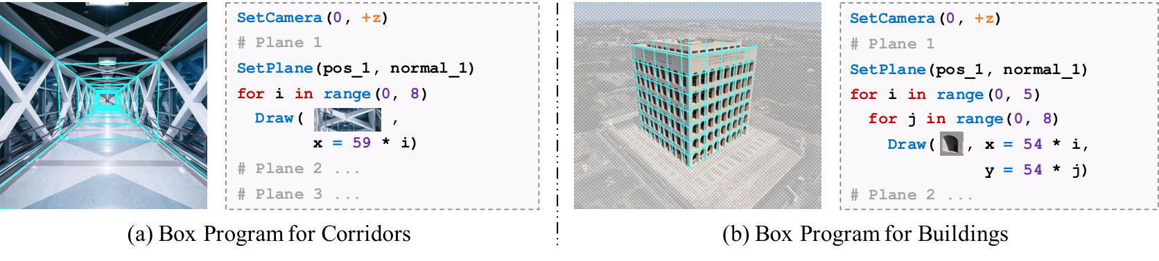
We start by describing the domain-specific language (DSL) that we use to express the multiple planes in the scene and the regularity structure on individual planes, namely the box programs. We assume these planes are faces of a 3D box. Take Fig. 2a as an example: the corridor is composed of four planes, each containing visually regular patterns.

Table 1 specifies the DSL, and Fig. 2 shows sample programs. A box program consists of two parts: camera parameters and programs for individual planes. A plane program first sets the plane’s surface normal, then specifies a sub-program defining the regular 2D pattern on the plane. These patterns utilize the primitive Draw command, which places patterns at specified 2D positions. Draw commands appear in For-loop statements that characterize the regularity of each plane.

3.2 Box Program Fitness

Given an input image, our goal is to segment the image into different planes, estimate their surface normals relative to the camera, and infer the regular patterns. We treat this problem as seeking a program $P$ that best fits the input image $I$ . We first define the fitness of a program $P$ by measuring how well $P$ reconstructs $I$ . Recall that a box program $P$ is composed of multiple plane programs, each of which defines the regular pattern on a plane as well as its position and orientation in 3D. Combined with camera parameters, we can use parameters of each plane program to rectify the corresponding plane, resulting in images without perspective effects $\{J_{1},J_{2},\cdots,J_{k}\}$ , where $k$ is the number of planes described by $P$ .

For each plane $i$ , we compute its fitness score by comparing its rectified image $J_{i}$ and the corresponding plane program block, denoted as $Q_{i}$ . The fitness score is defined in a similar way as in the Perspective Plane Program Induction framework [21]. Specifically, executing $Q_{i}$ produces a set of 2D coordinates $C_{i}$ that can be interpreted as the centers of each visual element, such as the center of the lights on the ceiling in Fig. 2a. Since $Q_{i}$ contains a nested loop of up to two levels, we denote the loop variable for each For loop as $a$ and $b$ . Thus, each 2D coordinate in $C_{i}$ can be written as a function of $a$ and $b$ , $c(a,b)\in\mathbb{R}^{2}$ . The fitness score $F$ is defined as

F=-\sum_{a,b}\left[\left\|J_{i}[c(a,b)]-J_{i}[c(a+1,b)]\right\|_{2}^{2}+\left\|J_{i}[c(a,b)]-J_{i}[c(a,b+1)]\right\|_{2}^{2}\right],

(1)

where $\|\cdot\|_{2}$ is the $\mathcal{L}_{2}$ norm and $J_{i}[c(a,b)]$ denotes the patch centered at 2D coordinates $c(a,b)$ . Since we only consider lattice patterns on individual planes, we implement this by first shifting $J_{i}$ leftward (or downward) by the ‘width’ (or ‘height’) of a lattice cell and then computing the pixel-wise difference between the shifted image and the original image $J_{i}$ . The overall program fitness of $P$ is the sum of the fitness function for all planes.

3.3 3D Box Priors and the Role of Visual Cues

A naïve way to find the best-fit program $P$ is to enumerate all possible plane segmentations of the input image $I$ and rank all candidates by the fitness score (Eq. 1). However, the complexity of this naïve method scales exponentially in the number of planes. Instead, we propose to consider first, the box prior, which constrains the plane segmentation of the image and, second, visual cues that help to guide the search. Specifically, we impose the following box prior:

•

For an inner view of a box, e.g., a corridor as in Fig. 2a, our box program models four planes: two side walls, the floor, and the ceiling. For images with a far plane, we will segment the far plane but do not use programs to model it, as most far planes do not contain a regular structure.
•

For an outer view of a box, e.g., a building as in Fig. 2b, our box program models the two side walls as two planes. We do not model the roof as, in most images, the roof is either nonvisible or very small in size.

Below, we show how to use visual cues to guide the search for box programs. We focus on the inner view case, and include details for the outer view case in the supplemental material. The full search process is illustrated in Fig. 3, and consists of four steps. First, we use pre-trained neural networks to detect the vanishing point and the 2D wireframes line segments from the image. We also filter out invalid wireframe segments. Next, we generate a set of candidate plane segmentations based on the detected wireframe segments. Then, for each segmented plane, we seek the program that best describes the plane structure. Finally, we rank all candidate plane segmentations by the fitness score.

Step 1: Visual cue detection.

Following the box prior, all inner views of a box contain a single vanishing point and four intersection lines that are the intersection between the two walls, the ceiling, and the floor in 3D. These intersection lines will be projected onto the image plane as four lines that intersects at the vanishing point. We use this property to constrain the candidate plane segmentation. Leveraging vanishing point information for inferring box structures of scenes has also been studied in [15].

Given an input image (Fig. 3a), we apply NeurVPS [47] to detect the vanishing point and L-CNN [48] to extract wireframes in the image. We use the most confident prediction of NeurVPS as the vanishing point $\mathit{vp}\in\mathbb{R}^{2}$ , which is a 2D coordinate on the image plane. Each wireframe segment is represented as a segment $AB$ on the image, from $(x^{A},y^{A})$ to $(x^{B},y^{B})$ , as illustrated in Fig. 3b. Next, we filter out wireframe segments whose length is smaller than a threshold $\delta_{1}$ or whose extension does not cross a neighbourhood centered at $\mathit{vp}$ with radius $\delta_{2}$ . The remaining wireframe segments, denoted by the set $\mathit{WF}$ , are illustrated in Fig. 3c.

Step 2: Plane segmentation.

We then enumerate all combinations of four wireframe segments from $\mathit{WF}$ . As these wireframe segments $s_{i}=[(x_{i}^{A},y_{i}^{A}),(x_{i}^{B},y_{i}^{B})],i=1,2,3,4$ may not intersect at a single point, we compute a new vanishing point $\mathit{vp}^{*}$ that minimizes $\sum_{i}\mathit{dist}(\mathit{vp}^{*},s_{i})$ , where $\mathit{dist}$ is the distance between the point $\mathit{vp}^{*}$ and the line containing segment $s_{i}$ . Next, we connect the new vanishing point $\mathit{vp}^{*}$ and the farther end of each $s_{i}$ to get four rays. These four rays partition the image into four parts, which we treat as the segmentation of four planes, as illustrated in Fig. 3d.

Step 3: Plane rectification and regularity inference.

Fixing the camera at the world origin, pointing in the + $z$ direction, we then compute the 3D position and surface normal of each plane. As shown in Fig. 1, because the distance between camera and the corridor is coupled with the focal length of the camera, here we use a fixed focal length of $f=35\mathrm{mm}$ ^*^* * Following common practice, we also fix other camera intrinsic properties: optical center to $(0,0)$ , skew factor to $0$ , and pixel aspect ratio to $1$ .. Based on these assumptions, the four rays can unambiguously determine the 3D positions and surface normals of four planes. The proof can be found in the supplemental material.

Based on the inferred surface normal, we can rectify each plane, yielding a set of rectified images $\{J_{1},J_{2},\cdots,J_{4}\}$ . For each rectified plane, we search for the best plane program that describes it, based on the fitness function Eq. 1. The inferred plane regularity structures are shown in Fig. 3e.

Step 4: Box program ranking.

We sum up the fitness score for four planes in each candidate segmentation as the overall program fitness. We use this score to rank all candidate segmentations, and choose the program with the highest fitness to describe the entire image.

3.4 Program-Guided Image Manipulation

The inferred box program enables 3D-aware interactive image manipulation: inpainting missing pixels, changing camera parameters , and extrapolating the image content. Lying at the core of these applications is a program-guided PatchMatch algorithm.

Our program-guided PatchMatch augments the PatchMatch algorithm [4] by enforcing the regularity on each plane. Consider the task of inpainting missing pixels on the wall of a building in Fig. 4. Taking a corrupted image as input (Fig. 4a), we infer the box program from the undamaged pixels (Fig. 4b). The inferred box program explains the plane segmentation and the regularity pattern on each plane. For each plane that contains missing pixels, we can first rectify the corrupted plane as shown in Fig. 4c. Since the plane program on this plane will partition the image with a lattice, we construct a “shift map”, illustrated as Fig. 4d, which represents the relative position of each pixel to the center of the lattice cell that this pixel lies in, normalized to $[-0.5,0.5]$ .

In PatchMatch, the similarity $\mathit{sim}(p,q)$ between pixel $p$ and pixel $q$ is computed as a pixel-level similarity $\mathit{sim}_{\mathrm{pixel}}$ between two patches centered at $p$ and $q$ , with a constant patch size $\delta_{\mathrm{pm}}$ . We add another term to this similarity function:

\mathit{sim}(p,q)\triangleq\mathit{sim}_{\mathrm{pixel}}+\mathit{sim}_{\mathrm{reg}}=\mathit{sim}_{\mathrm{pixel}}-\lambda_{\mathrm{reg}}\|\mathrm{wraparound}(\mathit{smap}[p]-\mathit{smap}[q])\|^{2}_{2},

(2)

where $\lambda_{\mathrm{reg}}$ is a hyperparameter that controls the weight of the regularity enforcement. $\mathrm{abs}$ is the absolute value function. The shift-map term measures whether two pixels $p$ and $q$ correspond to the same location on two (possibly different) repeating elements on the plane. We “wrap around” shift map distance by $\mathrm{wraparound}(\mathbf{x})\equiv\max(1-\mathbf{x},\mathbf{x})$ , as the top-left corner and the bottom-right corner of a cell also matches. Thus, the PatchMatch algorithm will choose the pixel based on both pixel similarity and regularity similarity to fill in the missing pixels (Fig. 4e).

4 Experiments

For evaluation, we introduce two datasets, and then apply box programs to vision and graphics tasks on these datasets, including plane segmentation (Sec. 4.1), image inpainting and extrapolation (Sec. 4.2), and view synthesis (Sec. 4.3).

Dataset.

We collect two datasets from web image search engines for our experiments, a 44-image Corridor Boxes dataset and a 42-image Building Boxes dataset. These correspond to the inner view and the outer view of boxes, respectively. For both datasets, we manually annotate the plane segmentations by specifying edges of the boxes. For corridor images, we also create a mask for the far plane. For building images, we supplement the subject segmentation (i.e., the building of interest) to the dataset annotation.

4.1 Plane Segmentation

Because BPI develops a 3D understanding of the scene in the process of inferring the box program under perspective effects, an immediate application is single-image plane segmentation. Note that BPI performs this task by jointly inferring the perspective effects and the pattern regularity, in contrast to supervised learning approaches that train models with direct supervision, such as [23]. The core intuition is that the correct plane segmentation leads to the program that best describes each segmented plane in terms of repeated visual elements.

Baselines.

We compare our method with two baselines: Huang et al. [16] and PlaneRCNN [23]. Huang et al. [16] first uses VLFeat [35] to detect vanishing points and line segments. It then generates a soft partition of the image into multiple parts by the support lines. PlaneRCNN is a learning-based method for plane segmentation. It uses a Mask-RCNN-like pipeline [14] and is trained on ScanNet [6].

Method	CrdO	CrdC	BldO	BldC
Huang et al. [16]	0.30	0.30	0.73	0.69
PlaneRCNN	0.52	0.52	0.63	0.63
BPI (Ours)	0.84	0.84	0.86	0.86

Table 2: Plane segmentation results in IoU between detected and groundtruth planes. BPI outperforms both baselines on both original (CrdO, BldO) and corrupted images (CrdC, BldC).

Metrics.

The output of each model is a set of masks indicating the segmented planes. We compare these with the ground-truth masks by computing the best match between two sets of masks, where the matching metric is the intersection over union (IoU). We then report the average IoU of all predicted masks. For corridor images, we exclude pixels in the far plane region during evaluation. Because we wish to use the plane segmentation to aid in image manipulation tasks such as image inpainting, we evaluate all methods on both original images (CrdO, BldO) and corrupted images (CrdC, BldC).

Results.

Fig. 5 and Table 2 show that BPI consistently outperforms the baselines on both corridor and building images. The baselines fail to detect planes when they contain complex structures and patterns.

4.2 Image Inpainting

The inferred box programs support 3D-aware and regularity-preserving image manipulation, because they provide information on both what the perspective effects are and how the visual element repeats. To test BPI’s performance on such tasks, we generate a dataset of corrupted images by randomly masking out regions of images from our two datasets.

Metrics.

We use four metrics: pixel-level $\mathcal{L}_{1}$ distance, peak signal-to-noise ratio (PSNR), structural similarity index (SSIM) [37], and a learned perceptual metric LPIPS [45]. Following standard practice [28, 2], we compute PSNR and SSIM on image luma, and compute $\mathcal{L}_{1}$ distance and LPIPS directly on RGB values.

Baselines.

We compare our model against both learning-based GatedConv [44] and three non-learning-based algorithms: PatchMatch [4], Image Melding [7], and Huang et al. [16]. All three non-learning algorithms are patch-based. Image Melding allows additional geometric and photometric transformations on patches. Huang et al. [16] first segments the image into different planes and augments a standard PatchMatch procedure with the plane rectification results.

	Corridors				Buildings
Method	$\mathcal{L}_{1}$ Mean $\downarrow$	PSNR $\uparrow$	SSIM $\uparrow$	LPIPS $\downarrow$	$\mathcal{L}_{1}$ Mean $\downarrow$	PSNR $\uparrow$	SSIM $\uparrow$	LPIPS $\downarrow$
PatchMatch	53.12	31.55	0.9872	0.0215	34.88	32.99	0.9896	0.0072
Image Melding	58.50	30.54	0.9880	0.0174	49.10	30.42	0.9890	0.0134
Huang et al. [16]	51.88	31.41	0.9869	0.0177	26.10	34.87	0.9917	0.0049
GatedConv	44.98	32.32	0.9883	0.0153	55.31	29.54	0.9866	0.0112
BPI (Ours)	38.45	34.21	0.9892	0.0170	26.43	34.86	0.9913	0.0054

Table 3: We compare BPI-guided PatchMatch with both patch-based and learning-based methods on the task of image inpainting.

\uparrow

indicates that the higher the number, the better. Bold indicates models that are indistinguishable with the best one under that metric with a linear mixed model. See text for details.

Results.

The results are summarized in Table 3 and Fig. 6. Here we run linear mixed models between each pair of methods and, for each metric, we mark in bold all methods that are indistinguishable with the best one. All $p$ -values are in the supplementary material. Our method outperforms baselines on corridor images and achieves comparable results on building images with Huang et al. [16]. As discussed in Sec. 4.1, Huang et al. [16] relies on straight lines on the plane to segment and rectify the image, so it works well on planes with a plethora of such features. Huang et al. [16] tends to fail on images without dense straight lines on the plane (rows 3-4 of Fig. 6). On corridor images, beyond producing high-fidelity inpainting results, our regularity-aware PatchMatch process preserves the structure of the scene, such as the light on the ceiling in row 1 of Fig. 6.

Image extrapolation.

Beyond inpainting missing pixels, our regularity-aware algorithm can extrapolate the box structure. Here, on the Building Boxes dataset, we show that our model can make the building taller or wider. The input to the model is a foreground mask of the building and the target region to be filled with the extrapolated building. We compare our method with four baselines: Content-Aware Scaling in Adobe Photoshop, Kaspar et al. [18], Huang et al. [16] and InGAN [33]. For content-aware scaling, we first select the foreground mask and then scale it so that it fills the target region. For both Kaspar et al. [18] and InGAN, we extract the bounding box of the foreground building and use it as the input. The model generates a new image that is 1.5x larger. For Huang et al. [16], we cast the extrapolation problem as inpainting the target region.

As shown in Fig. 7, Content-Aware Scaling is unaware of perspective effects and fails to preserve the lattice structure in the image. It also cannot generate new visual elements such as windows. Both Kaspar et al. [18] and InGAN do not preserve existing pixels when extrapolating the image. Kaspar et al. [18], as a texture synthesis method, also ignores the two-plane structure when generating the new image. While InGAN is able to capture the visual elements, it does not follow the lattice pattern during synthesis. Huang et al. [16] can inpaint small local areas as in Fig. 6, but does not follow the regular structure when inpainting a large area. In contrast, BPI preserves both the plane structure of the building and the lattice pattern on each side.

Quantitatively, we randomly select 12 images, and ask 15 people to rank the outputs of different methods. We collected $12\times 15=180$ responses. The preference for the models are: Ours( $61\%$ ), Content-Aware Scaling( $16\%$ ), Kaspar et al. [18] ( $2\%$ ), InGAN( $16\%$ ), and Huang et al. [16] ( $5\%$ ).

4.3 View Synthesis

As our inferred box programs captures a holistic 3D scene representation, we can synthesize novel views of the scene from a single image. We compare different models on the Corridor Boxes dataset. We consider three types of camera movement: 1) “step into the corridor”, 2) “step back in the corridor”, and 3) “step back in the corridor, pan leftward, and tilt upward”. All trajectories generate 5 frames. Detailed parameters are included in the supplemental material. Note that in both trajectories that involve “stepping back”, the algorithm must synthesize pixels unseen in the original image. For our BPI, we run our program-guided PatchMatch to extrapolate the planes and synthesize pixels that are outside the input view frustum.

Results.

We compare images generated by our BPI and by SynSin [38] in Fig. 8. The arrow on the input shows camera movement. As our method can generate a corridor of an arbitrary length, we see significantly fewer artifacts when the camera movement is large, compared with SynSin. Note that even in the first columns where the camera movement is small, the pixels synthesized by SynSin that are outside the original view frustum already fail to preserve the regular structure.

For a quantitative comparison, we randomly select 20 images, generate synchronized videos of the results produced by our method and by SynSin on all three camera trajectories, and ask 10 people to rank the outputs. We collected $20\times 3\times 10=600$ responses. For the three different trajectories, $100\%$ , $94\%$ , and $99.5\%$ of the responses prefer our result to that by SynSin, respectively.

4.4 Failure Case

Fig. 9 shows three main failure cases of our model. First, our model might misdetect vanishing points and wireframe segments, as illustrated in (a), where the model missed the wireframe between the floor and the right plane (detected wireframes shown as red lines). A second type of failure can occur when the image has a solid color plane. Illustrated in (b), our model segments the pure white part of the floor as part of the left/right planes. Finally, the inference might fail due to irregular planes, as shown in (c), where the buildings on the left do not form a rectangular plane. These issues could be mitigated with light user interaction, such as specifying wireframes.

5 Conclusion

We have presented Box Program Induction (BPI), a framework for inferring program-like representations that model the regular texture and patterns in 2D planes and the 3D posing of these planes, all from a single image. Our model assumes a box prior, which constrains the plane segmentation of the image, and uses visual cues to guide the inference. The inferred box program enables 3D-aware interactive image editing, such as inpainting, extrapolation, and view synthesis. Currently, our algorithm assumes that the full image can be partitioned into planes with regular structures. Future research may consider integrating models that can handle the presence of irregular image regions.

Broader Impact

This paper presents an improved interactive image manipulation algorithms, which helps visual artists, photographers, and normal users who wants to perform content-aware and 3D-aware edits to their images. Moreover, our algorithm only use pixels from the input image itself during editing, which minimizes the biases coming from external sources. However, misuses of our algorithms can generate fake images that affect image forensics.

Acknowledgements

This work is supported by the Center for Brains, Minds and Machines (NSF STC award CCF-1231216), NSF #1447476, ONR MURI N00014-16-1-2007, and IBM Research. Work was done while Jiajun Wu was a visiting researcher at Google Research.

References

Ashikhmin [2001] Michael Ashikhmin. Synthesizing Natural Textures. In I3D, 2001.
Ballé et al. [2017] Johannes Ballé, Valero Laparra, and Eero Simoncelli. End-to-end Optimized Image Compression. In ICLR, 2017.
Ballester et al. [2001] Coloma Ballester, Marcelo Bertalmio, Vicent Caselles, Guillermo Sapiro, and Joan Verdera. Filling-in by Joint Interpolation of Vector Fields and Gray Levels. IEEE TIP, 10(8):1200–1211, 2001.
Barnes et al. [2009] Connelly Barnes, Eli Shechtman, Adam Finkelstein, and Dan Goldman. PatchMatch: A Randomized Correspondence Algorithm for Structural Image Editing. ACM TOG, 28(3):24, 2009.
Beltramelli [2018] Tony Beltramelli. Pix2Code: Generating Code from a Graphical User Interface Screenshot. In EICS, 2018.
Dai et al. [2017] Angela Dai, Angel X. Chang, Manolis Savva, Maciej Halber, Thomas Funkhouser, and Matthias Nießner. ScanNet: Richly-Annotated 3D Reconstructions of Indoor Scenes. In CVPR, 2017.
Darabi et al. [2012a] Soheil Darabi, Eli Shechtman, Connelly Barnes, Dan B Goldman, and Pradeep Sen. Image Melding: Combining Inconsistent Images using Patch-based Synthesis. In SIGGRAPH, 2012a.
Darabi et al. [2012b] Soheil Darabi, Eli Shechtman, Connelly Barnes, Dan B. Goldman, and Pradeep Sen. Image melding: combining inconsistent images using patch-based synthesis. ACM TOG, 31:82:1–82:10, 2012b.
Deng et al. [2017] Yuntian Deng, Anssi Kanervisto, Jeffrey Ling, and Alexander M Rush. Image-to-Markup Generation with Coarse-to-Fine Attention. In ICML, 2017.
Efros and Freeman [2001] Alexei A. Efros and William T. Freeman. Image Quilting for Texture Synthesis and Transfer. In SIGGRAPH, 2001.
Ellis et al. [2018] Kevin Ellis, Daniel Ritchie, Armando Solar-Lezama, and Josh Tenenbaum. Learning to Infer Graphics Programs from Hand-Drawn Images. In NeurIPS, 2018.
Ganin et al. [2018] Yaroslav Ganin, Tejas Kulkarni, Igor Babuschkin, S. M. Eslami, and Oriol Vinyals. Synthesizing Programs for Images Using Reinforced Adversarial Learning. In ICML, 2018.
He and Sun [2012] Kaiming He and Jian Sun. Statistics of Patch Offsets for Image Completion. In ECCV, 2012.
He et al. [2017] Kaiming He, Georgia Gkioxari, Piotr Dollár, and Ross Girshick. Mask R-CNN. In ICCV, 2017.
Hedau et al. [2009] Varsha Hedau, Derek Hoiem, and David Forsyth. Recovering the Spatial Layout of Cluttered Rooms. In CVPR, 2009.
Huang et al. [2014] Jia-Bin Huang, Sing Bing Kang, Narendra Ahuja, and Johannes Kopf. Image Completion using Planar Structure Guidance. ACM TOG, 33:129:1–129:10, 2014.
Iizuka et al. [2017] Satoshi Iizuka, Edgar Simo-Serra, and Hiroshi Ishikawa. Globally and Locally Consistent Image Completion. ACM TOG, 36(4):107, 2017.
Kaspar et al. [2015] Alexandre Kaspar, Boris Neubert, Dani Lischinski, Mark Pauly, and Johannes Kopf. Self Tuning Texture Optimization. CGF, 34(2):349–359, 2015.
Li et al. [2017] Jun Li, Kai Xu, Siddhartha Chaudhuri, Ersin Yumer, Hao Zhang, and Leonidas Guibas. GRASS: Generative Recursive Autoencoders for Shape Structures. ACM TOG, 36(4):52, 2017.
Li et al. [2019] Manyi Li, Akshay Gadi Patil, Kai Xu, Siddhartha Chaudhuri, Owais Khan, Ariel Shamir, Changhe Tu, Baoquan Chen, Daniel Cohen-Or, and Hao Zhang. GRAINS: Generative Recursive Autoencoders for INdoor Scenes. ACM TOG, 38(2):12:1–12:16, 2019.
Li et al. [2020] Yikai Li, Jiayuan Mao, Xiuming Zhang, William T. Freeman, Joshua B. Tenenbaum, and Jiajun Wu. Perspective Plane Program Induction from a Single Image. In CVPR, 2020.
Liebowitz et al. [1999] David Liebowitz, Antonio Criminisi, and Andrew Zisserman. Creating Architectural Models from Images. CGF, 18(3):39–50, 1999.
Liu et al. [2019a] Chen Liu, Kihwan Kim, Jinwei Gu, Yasutaka Furukawa, and Jan Kautz. PlaneRCNN: 3D Plane Detection and Reconstruction From a Single Image. In CVPR, 2019a.
Liu et al. [2018] Guilin Liu, Fitsum A. Reda, Kevin J. Shih, Ting-Chun Wang, Andrew Tao, and Bryan Catanzaro. Image Inpainting for Irregular Holes Using Partial Convolutions. In ECCV, 2018.
Liu et al. [2019b] Yunchao Liu, Zheng Wu, Daniel Ritchie, William T. Freeman, Joshua B. Tenenbaum, and Jiajun Wu. Learning to Describe Scenes with Programs. In ICLR, 2019b.
Mao et al. [2019] Jiayuan Mao, Xiuming Zhang, Yikai Li, William T. Freeman, Joshua B. Tenenbaum, and Jiajun Wu. Program-Guided Image Manipulators. In ICCV, 2019.
Mellor et al. [2019] John FJ Mellor, Eunbyung Park, Yaroslav Ganin, Igor Babuschkin, Tejas Kulkarni, Dan Rosenbaum, Andy Ballard, Theophane Weber, Oriol Vinyals, and SM Eslami. Unsupervised Doodling and Painting with Improved SPIRAL. arXiv:1910.01007, 2019.
Merkle et al. [2007] Philipp Merkle, Aljoscha Smolic, Karsten Muller, and Thomas Wiegand. Multi-view Video Plus Depth Representation and Coding. In ICIP, 2007.
Nazeri et al. [2019] Kamyar Nazeri, Eric Ng, Tony Joseph, Faisal Qureshi, and Mehran Ebrahimi. EdgeConnect: Generative Image Inpainting with Adversarial Edge Learning. arXiv:1901.00212, 2019.
Niu et al. [2018] Chengjie Niu, Jun Li, and Kai Xu. Im2Struct: Recovering 3d Shape Structure from a Single Rgb Image. In CVPR, 2018.
Shaham et al. [2019] Tamar Rott Shaham, Tali Dekel, and Tomer Michaeli. SinGAN: Learning a Generative Model from a Single Natural Image. In ICCV, 2019.
Sharma et al. [2018] Gopal Sharma, Rishabh Goyal, Difan Liu, Evangelos Kalogerakis, and Subhransu Maji. CSGNet: Neural Shape Parser for Constructive Solid Geometry. In CVPR, 2018.
Shocher et al. [2019] Assaf Shocher, Shai Bagon, Phillip Isola, and Michal Irani. InGAN: Capturing and Remapping the “DNA” of a Natural Image. In ICCV, 2019.
Tian et al. [2019] Yonglong Tian, Andrew Luo, Xingyuan Sun, Kevin Ellis, William T. Freeman, Joshua B. Tenenbaum, and Jiajun Wu. Learning to Infer and Execute 3D Shape Programs. In ICLR, 2019.
Vedaldi and Fulkerson [2008] A. Vedaldi and B. Fulkerson. VLFeat: An Open and Portable Library of Computer Vision Algorithms. http://www.vlfeat.org/, 2008.
Wang et al. [2011] Yanzhen Wang, Kai Xu, Jun Li, Hao Zhang, Ariel Shamir, Ligang Liu, Zhiquan Cheng, and Yueshan Xiong. Symmetry Hierarchy of Man-Made Objects. CGF, 30(2), 2011.
Wang et al. [2004] Zhou Wang, Alan C. Bovik, Hamid R. Sheikh, and Eero P. Simoncelli. Image Quality Assessment: From Error Visibility to Structural Similarity. IEEE TIP, 13(4):600–612, 2004.
Wiles et al. [2020] Olivia Wiles, Georgia Gkioxari, Richard Szeliski, and Justin Johnson. SynSin: End-to-end View Synthesis from a Single Image. In CVPR, 2020.
Xiong et al. [2019] Wei Xiong, Zhe Lin, Jimei Yang, Xin Lu, Connelly Barnes, and Jiebo Luo. Foreground-Aware Image Inpainting. In CVPR, 2019.
Yan et al. [2018] Zhaoyi Yan, Xiaoming Li, Mu Li, Wangmeng Zuo, and Shiguang Shan. Shift-Net: Image Inpainting Via Deep Feature Rearrangement. In ECCV, 2018.
Yang et al. [2017] Chao Yang, Xin Lu, Zhe Lin, Eli Shechtman, Oliver Wang, and Hao Li. High-Resolution Image Inpainting Using Multi-Scale Neural Patch Synthesis. In CVPR, 2017.
Young et al. [2019] Halley Young, Osbert Bastani, and Mayur Naik. Learning Neurosymbolic Generative Models via Program Synthesis. In ICML, 2019.
Yu et al. [2018] Jiahui Yu, Zhe Lin, Jimei Yang, Xiaohui Shen, Xin Lu, and Thomas S Huang. Generative Image Inpainting with Contextual Attention. In CVPR, 2018.
Yu et al. [2019] Jiahui Yu, Zhe Lin, Jimei Yang, Xiaohui Shen, Xin Lu, and Thomas S Huang. Free-Form Image Inpainting with Gated Convolution. In ICCV, 2019.
Zhang et al. [2018] Richard Zhang, Phillip Isola, Alexei A. Efros, Eli Shechtman, and Oliver Wang. The Unreasonable Effectiveness of Deep Networks As a Perceptual Metric. In CVPR, 2018.
Zhou et al. [2018] Yang Zhou, Zhen Zhu, Xiang Bai, Dani Lischinski, Daniel Cohen-Or, and Hui Huang. Non-Stationary Texture Synthesis by Adversarial Expansion. ACM TOG, 37(4):49, 2018.
Zhou et al. [2019a] Yichao Zhou, Haozhi Qi, Jingwei Huang, and Yi Ma. NeurVPS: Neural Vanishing Point Scanning via Conic Convolution. In NeurIPS, 2019a.
Zhou et al. [2019b] Yichao Zhou, Haozhi Qi, and Yi Ma. End-to-end Wireframe Parsing. In ICCV, 2019b.

Supplemental Material

This supplementary document is organized as the following. First, in Appendix A, we show the mathematical details of how to reconstruct the 3D positions and surface normal vectors of different planes based on the plane segmentation for a box’s inner views (see Appendix B for outer views). Second, in Appendix B, we present the Box Program Induction (BPI) applied to outer views of boxes (details on BPI applied to inner views are in the main text). Next, in Appendix C, we discuss the implementation details of BPI. Finally, we present more qualitative results on box program induction, plane segmentation, image inpainting, and image extrapolation in Appendix D.

Appendix A Plane Reconstruction from Segmentation in Inner Views

In an inner view of a box, we use the plane segmentation of the input image to determine the 3D positions and surface normal vectors of four planes. The plane segmentation is represented as four rays starting from the detected vanishing point. Our reconstruction assumes a pinhole camera model with no lens distortion, as illustrated in Fig. 10a.

We start by defining the 3D coordinate system. We define the position of the camera pinhole $O$ as origin of the coordinate system. We also define the optical axis of the camera (i.e., the ray from the center of the image plane $\Pi^{\prime}$ to $O$ ) as the $+z$ axis.

$V^{\prime}$ denotes the vanishing point shown on the image plane. Four rays starting from $V^{\prime}$ will intersect with the image boundary at four points $\{I^{\prime}_{k}\mid k=1,2,3,4\}$ . The line segments $\{V^{\prime}I^{\prime}_{k}\mid k=1,2,3,4\}$ , namely the intersection line segments, are 2D projections of the intersection lines in 3D, between four planes. We also denote these 3D intersections lines as $\{I_{k}E_{k}\mid i=1,2,3,4\}$ , where $I_{k}$ is the corresponding 3D projection of $I^{\prime}_{k}$ , and $E_{k}$ is the 3D projection of an arbitrary point on the 2D line segment $V^{\prime}I^{\prime}_{k}$ . Thus, all lines $\{I^{\prime}_{k}I_{k}\mid k=1,2,3,4\}$ should intersect at the optical center $O$ .

As can be seen in Fig. 10a, the focal length (i.e. the distance between the image center and the optical center $O$ ) is correlated with the distance between $I_{k}$ and $O$ (i.e., the camera-to-subject distance)^†^† † Formally, we need three planes that are perpendicular to each other to determine the focal length based on the perspective effect. However, we have only two such planes here. See Liebowitz et al. [22] for a detailed discussion.. Moreover, the aspect ratio of the image sensor is correlated with the ratio between the sizes of four planes (i.e., the “aspect ratio” of the box). Thus, it is impossible to fully determine the focal length and the camera aspect ratio from this single image. Given this ambiguity, we assume the focal length to be 35mm and the aspect ratio to be 1, and then optimize for the equivalent distance between $I_{k}$ and $O$ .

To this end, we first consider the following property of vanishing point: the line $V^{\prime}O$ should be parallel with all 3D intersection lines $I_{k}E_{k}$ . Thus, we perform an orthographical projection of the inner view using a new optical axis $V^{\prime}O$ . This leads to a new image $\Pi^{\prime\prime}$ , as illustrated in Fig. 10b. The line segment $OI_{k}$ will also be projected onto $\Pi^{\prime\prime}$ as a line segment $OI^{\prime\prime}_{k}$ , and four intersection lines $I_{k}E_{k}$ will become four points on $\Pi^{\prime\prime}$ . Determining the distance between $O$ and $I_{k}$ is equivalent to determining the distance between $I^{\prime\prime}_{k}$ and $V^{\prime}$ on the new image plane $\Pi^{\prime\prime}$ .

Unfortunately, one can not fully determine the distance between $I^{\prime\prime}_{k}$ and $V^{\prime}$ , but only the ratio between $V^{\prime}I^{\prime\prime}_{1}$ and $V^{\prime}I^{\prime\prime}_{k},k=2,3,4$ , even if we have assumed the focal length and the aspect ratio. This is because this camera-to-subject distance is also correlated with the actual size of the box. Intuitively, a box that is close and small may look identical in the image as another box that is far but big. Thus, we will manually set the distance between $V^{\prime}$ and $I^{\prime\prime}_{1}$ to be 1 meter. It is important to note that, although we have manually set the focal length, the aspect ratio, and the camera-to-subject distance, these value of these parameters will not affect the plane rectification results. Moreover, they also have no influence on downstream tasks such as image inpainting.

With the position of $I^{\prime\prime}_{1}$ , we then determine the positions of $I^{\prime\prime}_{k},k=2,3,4$ , relative to the position of $I^{\prime\prime}_{1}$ . We use the following box prior: four planes of the box are either perpendicular or parallel to each other. Thus, on the orthographic image plane $\Pi^{\prime\prime}$ , the quadrilateral $I^{\prime\prime}_{1}I^{\prime\prime}_{2}I^{\prime\prime}_{3}I^{\prime\prime}_{4}$ should be a rectangle.

Now we use the 2D coordinates defined on the plane $\Pi^{\prime\prime}$ and centered at the vanishing point $V^{\prime}$ . Denote the coordinates of $I^{\prime\prime}_{k}$ on $\Pi^{\prime\prime}$ by $(x_{k},y_{k})$ , the slope of $I^{\prime\prime}_{1}I^{\prime\prime}_{2}$ by $u$ , and the slope of $I^{\prime\prime}_{2}I^{\prime\prime}_{3}$ by $v$ . Also denote the slope of $VI^{\prime\prime}_{k}$ by $w_{k},k=1,2,3,4$ , as illustrated in Fig. 10b. We have the following equation system:

\begin{cases}y_{k}=w_{k}x_{k};\;k=1,2,3,4&\text{($I^{\prime\prime}_{k}$ lies on the ray $VI^{\prime\prime}_{k}$.)}\\ y_{1}-y_{2}=u(x_{1}-x_{2})&\text{(definition.)}\\ y_{2}-y_{3}=v(x_{2}-x_{3})&\text{(definition.)}\\ y_{3}-y_{4}=u(x_{3}-x_{4})&\text{($I^{\prime\prime}_{1}I^{\prime\prime}_{2}$ is parallel to $I^{\prime\prime}_{3}I^{\prime\prime}_{4}$.)}\\ y_{4}-y_{1}=v(x_{4}-x_{1})&\text{($I^{\prime\prime}_{2}I^{\prime\prime}_{3}$ is parallel to $I^{\prime\prime}_{4}I^{\prime\prime}_{1}$.)}\\ x_{1}^{2}+y_{1}^{2}=1&\text{(camera-to-subject distance assumption.)}\\ uv=-1&\text{($I^{\prime\prime}_{1}I^{\prime\prime}_{2}$ and $I^{\prime\prime}_{2}I^{\prime\prime}_{3}$ are perpendicular to each other.)}\\ \end{cases}

This equation system allows us to solve for $u$ and $v$ unambiguously. In fact, there exists a closed-form solution to the values of $u$ and $v$ , which is independent of $(x_{k},y_{k})$ . After determining $u$ and $v$ , we can further compute the positions of $I^{\prime\prime}_{k}$ and thus the 3D positions of $I_{k},k=1,2,3,4$ .

During inference, we first compute the orthographic projection $\Pi^{\prime\prime}$ based on the detected vanishing point and the focal length. Next, by fixing the position of $I^{\prime\prime}_{1}$ , we solve for the other $I^{\prime\prime}_{k},k=2,3,4$ on the orthographic image. Finally, we project the solution back to the 3D space and determine the 3D positions and surface normal vectors for individual planes.

Appendix B Box Program Induction for Outer Views of Boxes

In this section, we present the box program induction for outer views of boxes. The whole process is almost identical to the inner view case, except that for an outer view, we only need to consider two planes (e.g., two side planes of a building), with the other planes being either non-visible or foreshortened severely. The full search process consists of four steps. First, we use pre-trained neural networks to detect the 2D wireframe line segments (but no vanishing points) from the image. We also filter out wireframe segments that are too short in length. Next, we generate a set of candidate plane segmentation maps by partitioning the image based on the detected wireframe segments. Then, for each segmented plane, we seek the program that best describes the regularity on each plane. Finally, we rank all candidate plane segmentations by the fitness score (defined in the main text).

Step 1: Visual cue detection.

Following the box prior, an outer view of a box contains only two planes. Therefore, there will be only one intersection line between these two planes (e.g., two walls of a building). We use L-CNN [48] to extract wireframes in the image. Next, we filter out wireframe segments whose length is smaller than a threshold $\delta_{1}$ . The remaining wireframe segments are denoted by the set $\mathit{WF}$ . Note that unlike the inner view case, we do not use vanishing point detection for outer views.

Step 2: Plane segmentation.

Next, we then extend every wireframe segment to a line. Each line will partition the input image into two parts, which we treat as the candidate plane segmentation of the image.

Step 3: Plane rectification and regularity inference.

Since we only have two planes, we cannot use the plane segmentation to fully reconstruct the positions and surface normal vectors of different planes. We run the Perspective Plane Program Induction (P3I) algorithm [21] on each plane to jointly infer the surface normal of each plane and its regularity structure.

Step 4: Box program ranking.

Identical to the inner view case, we sum up the fitness score for two planes in each candidate segmentation as the overall program fitness. We use this score to rank all candidate segmentations, and pick the program with the highest fitness to describe the entire image.

Appendix C Implementation Details

When filtering wireframes by length, we set $\delta_{1}=0.1\times\text{min}(w,h)$ , where $w,h$ are the width and height of the input image, respectively. Radius used to filter wireframes toward the detected vanishing point is $\delta_{2}=0.01\times\text{min}(w,h)$ . In the plane rectification step, we rectify the plane region to a $200\times 200$ image, on which we infer the regularity. We assume that objects repeat at least 3 times on each plane.

Appendix D Additional Results

Time complexity.

For the corridor dataset, statistically, each image contains 1,506 wireframe combinations on average. 46 programs are evaluated on each plane. Note that BPI reduces the search space significantly based on the box prior, so that the search can be done efficiently (23 $\times$ faster than without the box prior).

We also show the runtime of different algorithms on the task of plane segmentation (Table 4) and image inpainting (Table 5). The Image Melding [7] and Huang et al. [16] baselines are tested on a single machine with an Intel i7-6500U@2.5GHz CPU and 8GB RAM. All other baselines are tested on a single machine with an Intel E5-2650@2.20GHz CPU, a GeForce GTX 1080 GPU, and 8GB RAM.

Qualitative results.

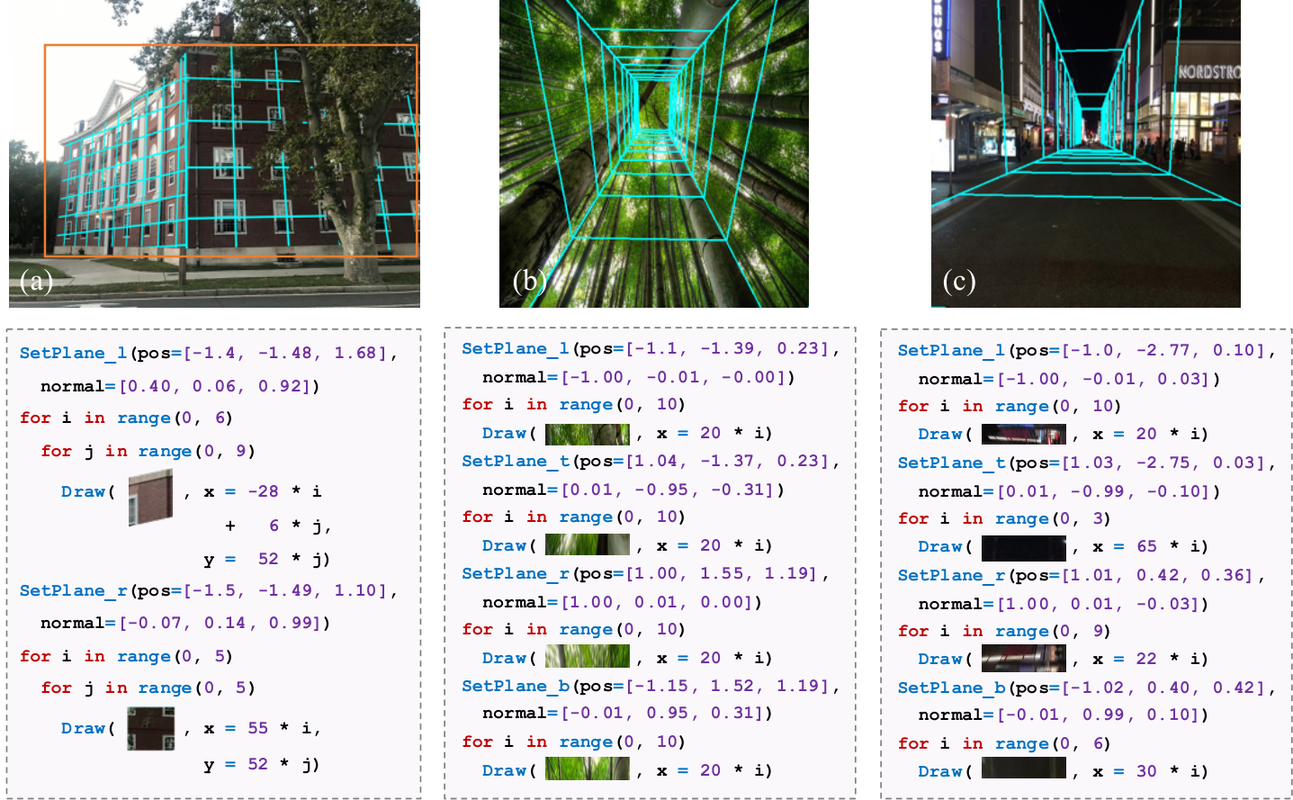
We supplement more results on box program induction (Fig. 11). Our model can be applied to less constrained images by allowing the user to specify the regular region. It also works for images where not all planes of a box exhibit regular patterns. Fig. 11 (i) shows example results. In (a), we run BPI on a user-specified region (the orange bounding box). BPI outputs a reasonable program even though the left plane is curved. We also show that our model can be applied to a broader class of images than buildings, such as the bamboo forest in (b), and the scene with irregular planes in (c).

We also provide more qualitative results for plane segmentation (Fig. 12), image inpainting (Fig. 13) and image extrapolation (Fig. 14).

	Huang et al. [16]	PlaneRCNN [23]	BPI (Ours)
Corridor Boxes	1.91s	0.14s	43.50s
Building Boxes	6.83s	0.76s	171.20s

Table 4: Runtime of different methods on the task of plane segmentation.

	PatchMatch [4]	Image Melding [7]	Huang et al. [16]	Gated Conv [44]	BPI (Ours)
Corridor Boxes	61.6s	1275.1s	18.9s	1.9s	20.1s
Building Boxes	122.1s	808.3s	64.4s	4.9s	41.4s

Table 5: Runtime of different methods on the task of image inpainting.