Temporal Surrogate Back-propagation for Spiking Neural Networks

Yukun Yang Affiliation: ECE Department Affiliation: UC Santa Barbara Affiliation: Santa Barbara, CA 93106 Email: yukunyang@ucsb.edu

Abstract

Spiking neural networks (SNN) are usually more energy-efficient as compared to Artificial neural networks (ANN), and the way they work has a great similarity with our brain. Back-propagation (BP) has shown its strong power in training ANN in recent years. However, since spike behavior is non-differentiable, BP cannot be applied to SNN directly. Although prior works demonstrated several ways to approximate the BP-gradient in both spatial and temporal directions either through surrogate gradient or randomness, they omitted the temporal dependency introduced by the reset mechanism between each step. In this article, we target theoretical completion and investigate the effect of the missing term thoroughly. By adding the temporal dependency of the reset mechanism, the new algorithm is more robust to learning-rate adjustments on a toy dataset but does not show much improvement on larger learning tasks like CIFAR-10. Empirically speaking, the benefits of the missing term are not worth the additional computational overhead. In many cases, the missing term can be ignored.

1 Introduction

SNN is believed as the 3^rd generation artificial intelligence, its potential is yet to be discovered. Despite the high power efficiency as compared with traditional ANN, the application is constrained by the low accuracy brought by SNN’s non-continuous spike behavior. How to boost SNN’s performance and find its suitable application scenarios are the main focuses of current researches.

2 Background

2.1 The Spiking Neuron Model

The discrete time leaky integrate-and-fire (LIF) model follows:

U^{(l+1)}[t+1]=U^{(l+1)}[t]\left(1-\frac{1}{\tau_{m}}\right)\left(1-S^{(l+1)}[t]\right)+\mathbf{W}^{(l)}a^{(l)}[t]

(1)

a^{(l+1)}[t+1]=a^{(l+1)}[t]\left(1-\frac{1}{\tau_{s}}\right)+\frac{1}{\tau_{s}}S^{(l+1)}[t+1]

(2)

S^{(l+1)}[t]=H\left(U^{(l+1)}[t]-\vartheta\right),H(x)=\begin{cases}0,~x<0\\ 1,~x>0\end{cases}

(3)

The compute graph is shown on the left side of Figure 1. We can safely substitute the variable $S$ by bringing the equation (3) into equations (1) & (2) and get:

U^{(l+1)}[t+1]=U^{(l+1)}[t]\left(1-\frac{1}{\tau_{m}}\right)\left[1-H\left(U^{(l+1)}[t]-\vartheta\right)\right]+\mathbf{W}^{(l)}a^{(l-1)}[t]

(4)

a^{(l+1)}[t+1]=a^{(l+1)}[t]\left(1-\frac{1}{\tau_{s}}\right)+\frac{1}{\tau_{s}}H\left(U^{(l+1)}[t+1]-\vartheta\right)

(5)

This leads our compute graph into the right side of Figure 1

Refer to caption — Figure 1: The two compute graphs

2.2 The Loss Function

Use Van Rossum distance with kernel $\epsilon$ to measure the difference between a desired output spike trains $\boldsymbol{d}$ and an actual output spike trains $\boldsymbol{S}$ :

L=\sum_{k=0}^{N_{t}}E_{t_{k}}=\sum_{k=0}^{N_{t}}\frac{1}{2}\left((\epsilon\ast\boldsymbol{d})[t_{k}]-(\epsilon\ast\boldsymbol{S})[t_{k}]\right)^{2}

(6)

3 Methods

According to the computation graph without variable $S$ , and follows the basic Back-propagate through time (BPTT) strategy, we can get:

\frac{\partial L}{\partial U^{(l)[t]}}=\underbrace{\frac{\partial L}{\partial a^{(l)[t]}}\frac{\partial a^{(l)[t]}}{\partial U^{(l)[t]}}}_{\textbf{Spatial}}+\underbrace{\frac{\partial L}{\partial U^{(l)[t+1]}}\frac{\partial U^{(l)[t+1]}}{\partial U^{(l)[t]}}}_{\textbf{Temporal}}

(7)

The activation based methods like SLAYER[1], STBP[2], SuperSpike[3], and ANTLR [4] choose different approaches to approximate the Spatial term. However, as for the Temporal part, we derived it based on equation (4) as following:

\frac{\partial U^{(l)[t+1]}}{\partial U^{(l)[t]}}=\left(1-\frac{1}{\tau_{m}}\right)\left\{\left[1-H\left(U^{(l)}[t]-\vartheta\right)\right]+\color[rgb]{1,0,0}{U^{(l)}[t]\left[-\frac{\partial H\left(U^{(l)}[t]-\vartheta\right)}{\partial U^{(l)}[t]}\right]}\color[rgb]{0,0,0}{}\right\}

(8)

The red colored term is missed in all previous works. This term is also ill-issdefined as the term ${\partial a^{(l)[t]}}/{\partial U^{(l)[t]}}$ in the Spatial term for the same reason: The derivative of $H(x)$ over $x$ is the Dirac delta function, which is zero almost everywhere and is infinity only when $x=0$ . However this term encodes an important dependency of membrane potential between different time steps. Like all previous works, we use the surrogate gradient method to approximate the Heaviside step function’s gradient:

H\left(U^{(l)}[t]-\vartheta\right)\approx\sigma\left.\left(U^{(l)}[t]-\vartheta\right)\right|_{T}=\frac{1}{1+e^{\frac{-\left(U^{(l)}[t]-\vartheta\right)}{T}}}

(9)

\frac{\partial H\left(U^{(l)}[t]-\vartheta\right)}{\partial U^{(l)}[t]}\approx\frac{1}{T}\left.\sigma\left(U^{(l)}[t]-\vartheta\right)\right|_{T}*\left(1-\sigma\left.\left(U^{(l)}[t]-\vartheta\right)\right|_{T}\right)

(10)

The new surrogate gradient term describes the timing dependency brought by the reset mechanism: When the membrane potential near the threshold, small perturbation towards threshold has potential to change the membrane potential of the next time-step dramatically.

4 Experiments

4.1 Toy Experimental Setup

We simulate a single neuron, with fixed random input spike current and fixed fictitious random target spike-trains. We use standard BP algorithm to train the neuron by 200 iteration. All parameters are concluded in the Table 1:

Table 1: Important parameters of the single neuron back-propagation experiment

#Input neuron	50	Desired spike-train $p$	1/20	$\tau_{m}$	6	Sigmoid $T$	0.3
#Time steps	100	Input spike-train $p$	1/10	$\tau_{s}$	2	Default lr	0.005

In the Table 1, variable $p$ means the probability of generating a spike on each time-step when initialize fictitious inputs or a target output spike-trains. As shown in the right side of Figure 2, the neuron’s output converged to the desired output successfully near the 30th iteration.

On the left side, we put four figures to show the four computing phases of gradients (All 200 iterations overlapped together). The Figure A is the difference between the current and the desired output. Then the difference is propagated to spike-trains in the Figure B. Since all previous spikes contribute to later current, the new graph gains a left tail on each spike compared to Figure A. By multiply the surrogate gradient of $\partial S/\partial U$ , the Figure B transit to the $grad_{u_{s}}$ shown in Figure C. Finally, the Figure D add the timing dependency with the missing term $grad_{u_{t}}$ mentioned above onto the $grad_{u_{s}}$ .

4.2 Toy Experiment Results

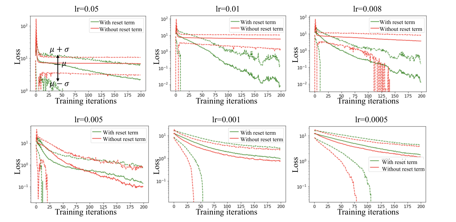
We repeat this toy experiment multiple times and record the loss curve. Figure 3 compares the loss curve before and after adding the reset term. The solid lines are averaged losses, and the dash lines are one standard deviations above/below the averages. After adding the reset term, the algorithm performs better when learning rate is $>0.005$ as shown on the first line of Figure 3, and has competitive performance with smaller learning rate.

4.3 Larger datasets

We conclude our current results in the Table 2. The parameters of the CNNs we used are shown in the Table 3 below:

Table 2: Performance comparison on larger datasets

Datasets	With reset term accuracy(%)	Without reset term accuracy(%)
NMNIST	99.29	99.28
MNIST	99.49	99.50
CIFAR10	88.96	88.98

Table 3: CNN’s parameters

Datasets	Network Size	Time steps
NMNIST	12C5-P2-64C5-P2	5
MNIST	15C5-P2-40C5-P2-300	30
CIFAR10	96C3-256C3-P2-384C3-P2-384C3-256C3-1024-1024	5

5 Conclusion and future works

In this short article. We add on the previous missed reset dependency between time steps using surrogate gradient. The new term shows better performance on the single neuron experiment when learning rate is larger than 0.005. However, on real datasets include MNIST, NMNIST and CIFAR-10, adding this reset dependency does not help.

References

[1] Sumit B Shrestha and Garrick Orchard. Slayer: Spike layer error reassignment in time. Advances in Neural Information Processing Systems, 2018.
[2] Yujie Wu, Lei Deng, Guoqi Li, Jun Zhu, and Luping Shi. Spatio-temporal backpropagation for training high-performance spiking neural networks. Frontiers in neuroscience, 12:331, 2018.
[3] Friedemann Zenke and Surya Ganguli. Superspike: Supervised learning in multilayer spiking neural networks. Neural computation, 30(6):1514–1541, 2018.
[4] Jinseok Kim, Kyungsu Kim, and Jae-Joon Kim. Unifying activation-and timing-based learning rules for spiking neural networks. Advances in Neural Information Processing Systems, 2020.