A Bounded Multi-Vacation Queue Model for Multi-stage Sleep Control 5G Base station

Investigations have demonstrated the convincing results that Bounded Multi-vacation Queue (BMV) schemes can beat N-policy and T-policy schemes in terms of system performance and reliability. As N-policy has only adjustable parameters of $K$ - the system buffer maximum quota, it has a bounded energy consumption rate and delay while BMV-policy can tune its $N_{v}$ (vacation amount limit) and $L_{v}$ (vacation length mean) across much wider ranges to guarantee an improved solution. Similarly T-policy can be treated as a single vacation(SV) policy, given a fixed $T$, results have shown that if being broken into multiple equally weighted vacations to make a BMV-policy scheme, the system would achieve a much smaller delay. Figure 1 coincides with paper  [1] that power consumption level fluctuates and delay increases with the increase of N. In this particular simulation, $\lambda=550$, $\mu=1000$,$K=50$,$power_{on}=130$,$power_{off}=75$. Results show that though $\rho=0.55$ and $ratio_{power}=0.5769$, the normalised energy consumption per bit for N-policy regardless of which $N$ is selected, goes much higher than $0.6$. The system has not been saturated in terms of energy conservation efficiency. As delay is a traditional QoS metric of a network system, we might also want the new scheme would outperform N-policy scheme in terms of processing speed. Given a bounded delay for N-policy as $[D_{min},D_{max}]$,solutions with BMV-policy can be easily founded that match the design criteria that consumes less energy while falls within the delay bounds. Two of them are depicted on the figure as examples.

Suppose in T-policy, the vacation length is $L_{v}$ and in BMV-policy, with the increase of $n$ (maximum number of vacations), $L^{BMV}_{v}=\frac{L_{v}}{n}$, cases where $n\in[1\ 7]$ are being executed and evaluated.Figure 2, shows that with the increase of $n$, the delay decreases while the energy level fluctuates.Based on the limited tested cases, $NE_{BMV}>NE_{T}$ with $NE$ stands for normalised energy while $D_{BMV}<NE_{T}$. Given a fixed delay bounds $[D_{min}\ D_{max}]$ imposed by N-policy, results show that BMV-policy can produce feasible solutions with higher energy savings.

• •

  The following work is the first to theoretically discuss multi-stage sleep control in the current state of art 5G Base station.

• •

  It bridges the mathematically theoretical analysis and the practical engineering problem by the validation of software simulation. Previous works in theoretical queuing analysis rarely endeavor to go through thorough experimental tests. Neither have works in mobile engineering set forth to develop an analysis from brand new.

• •

  It treats the system design problem as an optimal control problem considering the trade-off between delay and energy consumption and provides sound analysis against both of these system metrics. Most of the new queuing analysis are devised to evaluate the delay metrics solely and for those to have evaluated the cost metric such as power consumption in a typical telecommunication system,this work is the first to propose a validated model for future accurate prediction.

• •

  It pioneers in evaluating the performance of the multi-stage sleep control 5G system using the validated model. Moreover, it is the first to evaluate tentatively the selective service rate scheme given a fixed pool within such system.

The queuing system consists of an intelligent server that can vacate whenever the queue is empty. The vacation duration is adjusted based on two parameter configurations. They are the maximum vacation number $N_{v}$ and the average vacation period $L_{v}$. To be more specific, the queue once in vacation mode will return to the workstation whenever a vacation period expires. If the queue is still empty, it will continue to next vacation period till the maximum vacation number is reached. Otherwise it will resume to work upon its return to the workstation. Please refer to Figure  3 for further illustration;

The input traffic model follows a Poisson distribution with an average rate of $\lambda$ and the service pattern follows an Exponential distribution with an average rate of $\mu$. For the time being, the power that the sever uses at vacation is $p_{s}$, the vacation length is uniform over all stages and the power that the server uses at work is $p_{a}$.

Assume that the sleeping sub-frame has a length of $L_{s}$ and the working sub-frame has a length of $L_{b}$. By design it is also assumed that the system starts with sleeping mode.

As there are at most $N_{v}$ sleeping periods, for the system to enter working mode after the first period, there must be at least 1 arrival during the first period. For the system to enter working mode after the $n$ period with $n\leq N_{v}$, there will be at least 1 arrival during the previous $(n-1)th$ period but none happens during the previous $(n-2)$ periods.

Let A presents the event that there is at least 1 arrival within time frame $iL_{v}$; B presents the event that there is at least 1 arrival within time frame $(i-1)L_{v}$; C presents the event that there is at least 1 arrival within time frame $iL_{v}-(i-1)L_{v}$ only, which is equivalent to the phenomena that packets start to arrive during $i^{th}$ sleeping period. Henceforth $C=A-B$. Further on, $P(C)=P(A)-P(B)$. The formula is constructed as :

Upon entering the working period, the system has a starting probability distribution of queue length which is $P_{init}=[p_{k}]\times K$ with $K$ is the maximum queue size. $p_{k}=\exp(-\lambda L_{v})\frac{{(\lambda L_{v})}^{k}}{k!}$

Assume the transition matrix is $P_{\mathrm{tran}}$,the formation of $P_{\mathrm{tran}}$ for current $M/M/1/K$ queue system can be extended from paper [1]. $P_{\mathrm{tran}}=[p_{i,j}]*[K\times K]$

$[P_{\mathrm{zero}}(k)\ P_{\mathrm{other}}(k)]=[0\ P_{\mathrm{other}}(k-1)]*P_{\mathrm{tran}}$

The special event that no arrival within the maximum number of vacation periods is analysed as below: The period between the end of the overall sleeping sub-frame and the beginning of server running period is labeled as $ilen$ - the idle length. As Poisson Distribution follows an individually independent Markovian pattern, $ilen$ is perceived as the inter-arrival time between the zero arrival and the first arrival minus the maximum overall sleeping sub-frame.

$L_{a}$ is the inter-arrival time for the first packet in the idle mode and $N_{L_{s}}$ is the number of arrivals within period $L_{s}$.

At the end of this inter-arrival time, the queue length probability distribution as $P_{\mathrm{init}}$ is $[0]\times K$ and $P_{\mathrm{init}}[1]=1$

Let the ratio $r=\frac{L_{s}}{L_{b}+L_{s}}$. Normalised energy per bit can be derived from $E_{i}=1-r+r*\frac{p_{s}}{p_{a}}$. $i<=N_{v}$ are the events where the server resume to work within the maximum amount of sleep frames. In these cases $L_{s}=i*L_{v}$ and $L_{b}+L_{s}=L_{b}+i*L_{v}$. Then $i=N_{v}+1$ is the event where the server has an idle stage between the sleeping sub-frame and the working sub-frame. In this case $L_{s}=N_{v}*L_{v}$ and $L_{s}+L_{b}=L_{b}^{\prime}+ilen+N_{v}*L_{v}$. Lastly the event for $i>N_{v}+1$ doesn’t exist. Let $NE$ be the acronym for normalised energy per bit, then.

where the probability of first arrival within $i^{th}$ vacation period $P_{L_{s}(i)}=\exp{-\lambda(i-1)L_{v}}-\exp{-\lambda iL_{v}}$.

Waiting time analysis borrows Little’s Theorem basic idea.The analysis is performed as decomposing the long term waiting time average for the system into two event cases: $A$ no arrival within the limited vacation time; $B$ no less than 1 arrival within the limited vacation time. It is easy to conclude that $P(A)=exp(-\lambda(N_{v}L_{v}))$ and $P(B)=1-P(A)$.

For event $B$, following Theorem 2, $W=\frac{\triangle\gamma_{B}}{\triangle\alpha_{B}}$. Here $\alpha_{B}$ the overall packet in queue number is equivalent to the number of packets that have been departed during an averaged running cycle as the running cycle only stops when all the packets in queue are out of the system. $\triangle\gamma_{B}=A_{s}+A_{b}$ where $A_{s}$ is the packet in-queue time summation during an averaged vacation cycle and $A_{b}$ is the packet in-queue time summation during an averaged busy cycle.

The conditional queue length when the system resumes to work is $L^{init}_{Q}=E(L_{Q}|N_{a}>0)=\frac{\sum_{i=1}^{K}iPinit(i)}{\sum_{i=1}^{K}Pinit(i)}$, where $N_{a}$ is the number of arrival.

The conditional queue length when the system is active at departure epoch $k$ is $P_{ql_{k}}=\frac{\sum_{i}P^{k}_{\mathrm{other}}(i)i}{\sum_{i}P^{k}_{\mathrm{other}}(i)}$ when $k=0$, $Pqlen=L^{init}_{Q}$,

$A^{i}_{b}$ is the packet in-queue time summation when the queue becomes empty at the $ith$ departure epoch for an averaged busy cycle.

The optimisation goal is to select an ideal $(L_{v},N_{v})$ pair from a feasible pool for a given input traffic rate $\lambda$, given a fixed service rate $\mu$.

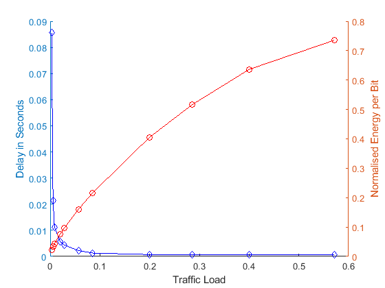
From Figure8 where $\mu=35025$, it can be concluded that with the increasing of traffic rate, the average waiting time is decreased. It is in alignment with Figure 6 in paper [6] in that with the increase of traffic intensity ($\rho\in[0\ 0.4]$ ), the normalised energy per bit rate increases and the normalised energy saving decreases.

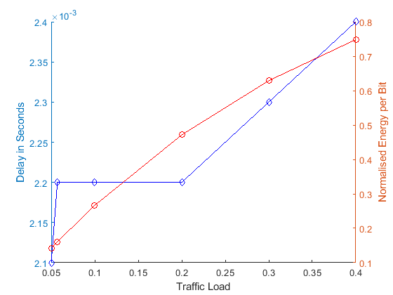
Next, scenario where the service rate can be varied is being studied. Assume the system supports dynamic frequency scaling (the system voltage is fixed) where $p=\alpha V^{2}f$ with $\alpha$ is a system specific constant. Let the data packet size to be uniform as $U$, which consumes $M$ clock cycles to process in total, then the time spent per packet is $MT_{clock}=\frac{M}{f_{clock}}$. It is inverse to the service rate so $\frac{f_{clock}}{M}=\mu$.That’s $f_{clock}=M\mu$. Hence $p=\beta\mu$ with $\beta=\alpha V^{2}M$.

For the ease of operation and observation, the configuration from Case 1 is borrowed where $\lambda=2000$,$\mu=35025$ and $p=234.2w$. Using the formula above, $\beta=0.00668665$. Suppose $\lambda=2000$ is fixed, increase the traffic load $(0.005\longrightarrow 0.4)$, results show that the energy consumption decreases as the traffic load decreases while the delay increases as the traffic load decreases. The former is reasonable because with less traffic load, the system enters sleep mode more often, the energy consumption is lessened henceforth. The latter is also reasonable as less traffic load means lower service rate and higher inter-departure time.

References

- [1] J.Chen, B.Sikdar and M.Hamdi. An Adpative N-policy Queueing System Design for Energy Efficient and Delay Sensitive Sensor Networks.Proceedings of the 2018 IEEE Global Communications Conference (GB2018),2018.
- [2] B.T.Doshi. Queueing systems with vacations - A survey. Queueing Systems,1986.
- [3] B.T.Doshi A Note in Stochastic Decomposition in a GI/G/1 Queue with Vacations or Set-up Times. Journal of Applied Probability,1985
- [4] X.Guo,S.Zhou,Z.Niu and P.R.Kumar. Optimal wake-up mechanism for single base station with sleep mode.Proceedings of the 2013 25th International Teletraffic Congress (ITC),2013
- [5] B.Debaillie,C.Desset and F.Louagie.Flexible and Future Proof Power Model for Cellular Base Stations. 2015 IEEE 81st Vehicular Technology Conference (VTC Spring)
- [6] M.Hrone, P.Jolma,P.Lahdekorpi and J.Moilanen. Energy Efficiency of 5G Mobile Network with Base Station Sleep Modes. 2017 IEEE Conference on Standards of Communications and Networking, 2017