A Distributed Privacy-Preserving Learning Dynamics in General Social Networks

Optimizing the decision-making process to maximize the expected reward is an essential problem for socialized individuals. Learning the best option for an isolated individual with time-invariant finite memory has been proved impossible in [14, 15]. Nevertheless, a common wisdom may suggest that interacting with each others to share the choices in the social group may contribute to the success of the learning process. Specifically, one can learn the experiences from its peers so as to avoid making similar mistakes in the decision-making process [16, 17]. Whereas the learning algorithms in early studies involve either sampling stage [18] or adopting stage [19], it is demonstrated in [20] that combining the two steps together could be a better learning strategy empirically. The two-staged learning strategy is then applied in sociology and economics [21, 22, 23], where the two stages are both crucial for the learning process. Our work is partially inspired by the recent work [4]. It investigates the dynamics of the two-staged learning strategy which entails global information as input, such that one in the social network can be aware of the choices of all the others. Unfortunately, single-hop social networks are not always available, whereas collecting the choices over a general (multi-hop) social network may induce considerable communication overhead. Hence, in this paper, one of our contributions is to study the learning dynamics in general social networks where the individuals interact with each other by multi-hop communications.

Privacy has emerged as one of the main concerns in machine learning research [24]. One choice is to apply cryptography-based methods, e.g., secure multi-party computation [25, 26] and homomorphic encryption [27, 28]. However, the cryptography-based methods may induce considerable computation overhead. Therefore, another branch of studies rely on the notion of Differential Privacy (DP) [29]. In the traditional global DP, data are first collected from their owners to a trusted third-party. When the data are queried, the aggregated result for the query is perturbed by the third-party before being released to the untrusted requesters [30, 31]. The application of the global DP in federated learning is investigated in [32]. In each iteration of FL, participants first submit their local models to a trusted central server, and the server then feeds a perturbed aggregation to the participants. The noise-adding (or perturbing) technique is also used in designing defense mechanisms against attacks to well trained prediction models. For example, [33] proposed to add noise to the prediction results of a target classifier so as to defend against black-box membership inference attacks. In [34], predictions are perturbed to poison the training objectives of model stealing attackers.

According to the definition of the global DP, it is used only when there is a trusted third-party to collect data from individual data owners and to protect their privacy in the meanwhile; however, the trustworthiness of the (central) third-party infrastructure may not be guaranteed, and we have to consider locally protecting the privacy of the data owners. To serve the above goal, local DP (LDP) is proposed as a distributed variant of DP. For example, in [8, 9], data owners add noise to (or perturb) the gradients calculated locally before reporting them to a central server where the perturbed gradients are aggregated to update the model parameters. In [10], the data owners add noise to the locally calculated model parameters and then upload them to an aggregation server. In [32, 35], LDP is applied to achieve user-level privacy preservation in FL, by letting users upload noised local models. In addition, LDP has also been applied in on-line decision-making problems where decisions on selecting among a group of unknown options are made according to the reward feedbacks of the options in an on-line manner. For example, in [11, 12, 13], a central decision maker makes selection decisions according to the perturbed observations on the rewards of the options. The above proposals all consider the privacy issue in a centralized learning process where multiple data owners need to report their private information (e.g., local gradients, model parameters or reward observations) to an untrusted central infrastructure. In contrast, we are interested in investigate the privacy issue in a decentralized learning process where multiple decision makers (i.e., agents) do not trust each other but have to share their private experience with each other for making decisions collaboratively.

As mentioned in Sec. I, selecting among a set of unknown option is a very common issue in daily life, while our aim is to utilize the collaboration among the individual decision makers (i.e., agents) in a social group and to guarantee the privacy of the individuals when they collaborate with each other. This idea actually is motivated by many real-world applications. For example,

• •

  Clinical trials. Suppose there is an illness with multiple treatments for patients (a.k.a., options) and a group of experimenters (a.k.a., agents) sequentially choose among the given treatments. The goal for the experimenters is to maximize the number of cured patients without prior knowledge about the effects of the treatments. On one hand, the experimenters can collaborate with each other by exchanging their experience; on the other hand, they are not willing to publish their current treatment in use, as doing so may induce the leakage of sensitive information such as the patients’ health conditions and genomes.

• •

  Procurement of financial products. In many economic scenarios, individuals (a.k.a., agent) need to make a sequence of decisions on selecting among different financial products (a.k.a., options). The individuals can share their latest adopted options with each other for common prosperity; nevertheless, an individual would not like to let others know its actual selection on the financial products, especially the trustworthiness of the other peers cannot be ensured.

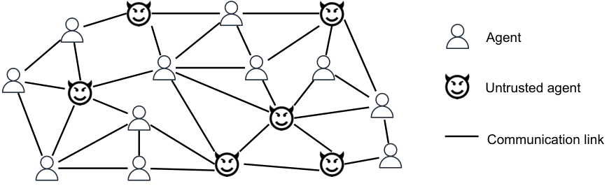
The privacy-preserving collaboration is also demanded in many other applications such as advertising, recommendation systems etc. Inspired by these application examples, we illustrate a social learning system in Fig. 1, where multiple agents in a social network can collaborate with each other by exchanging private experience through the communication links. Nevertheless, since the trustworthiness of the agents cannot be ensured, each of them has to preserve its privacy when collaborating with its peers. Note that we do not assume specific untrusted agents in this paper and we suppose each agent trusts none of the others. This system model will be formalized in the following.

We consider a social network represented by an undirected graph $\mathcal{G}=(\mathcal{N},\mathcal{E})$. $\mathcal{N}=\{1,2,\cdots,N\}$ denotes a set of $N$ agents while $\mathcal{E}$ denotes the set of the edges between the agents. For $\forall i,i^{\prime}\in\mathcal{N}$ and $i\neq i^{\prime}$, we have an edge $(i,i^{\prime})\in\mathcal{E}$ if they can exchange messages with each other. Let $\mathcal{N}_{i}=\{i^{\prime}\in\mathcal{N}\mid(i^{\prime},i)\in\mathcal{E}\}$ denote the neighbors of agent $i$ and $N_{i}$ be the size of $\mathcal{N}_{i}$ (i.e., the degree of agent $i$ in graph $\mathcal{G}$). Assume each agent $i$ initially is aware of $N_{i}$. Without loss of generality, we suppose $\mathcal{G}$ is a connected and non-bipartite graph. We assume that the network is well synchronized such that time can be divided into a sequence of rounds $r=1,2,\cdots,R$, each of which consists of $\Delta$ unit time slots. We adopt a relaxed CONGEST communication model, such that each agent is allowed to send only $\mathcal{O}(g(N))$ messages of $\mathcal{O}(\log N)$ bits over each edge in a slot ¹¹ 1 The formal definition of $g(N)$ will be given in Sec. III-D3. Informally, $g(N)$ is such that $\ln N<g(N)<N$ when $N$ is sufficiently large. We also suppose each agent has a privacy budget $\varepsilon$.

Suppose there are $M$ options $\mathcal{M}=\{1,\cdots,M\}$. Each option $j\in\mathcal{M}$ is associated with a random quality indicator $\Phi^{r}_{j}\in\{0,1\}$ in each round $r$ ²² 2 As will be shown later, our algorithm is readily compatible to quality indicators varying randomly across slots.. Specifically, we have $\Phi^{r}_{j}=1$ if option $j$ is “good” in round $r$ such that the agents choosing it can gain reward; otherwise, $\Phi^{r}_{j}=0$. For $\forall j\in\mathcal{M}$, $\Phi^{1}_{j},\Phi^{2}_{j},\cdots,\Phi^{R}_{j}$ are drawn independently and identically from an unknown Bernoulli distribution parameterized by $\eta_{j}$, i.e., $\Phi^{r}_{j}\sim\mathsf{Bernoulli}(\eta_{j})$, such that $\mathbb{P}[\Phi_{j}^{r}=1]=\eta_{j}$ and $\mathbb{P}[\Phi_{j}^{r}=0]=1-\eta_{j}$. Without loss of generality, suppose $\eta_{1}>\eta_{2}\geq\cdots\geq\eta_{M}$, such that the first option is the best.

During the learning process, the agents need to communicate with their neighbors for exchanging private information (i.e., their latest adoptions in our case), which entails a high demand on privacy preserving. For example, for each agent, if one of its neighbors is subverted by an adversary, the adversary may be able to eavesdrop on the private information shared by the agent. Therefore, in this paper, we consider a strong threat model by leveraging local privacy [6, 7], assuming that each agent trusts none of the others (especially its neighbors).

As introduced in Sec. I, the social learning algorithm proceeds iteratively in rounds $r=1,2,\cdots$. Let $X_{i,j}^{r}\in\{0,1\}$ be a binary variable indicating if agent $i$ adopts option $j$ in round $r$. We assume that each agent $i$ adopts at most one option in each round such that $\sum^{M}_{j=1}X^{r}_{i,j}\leq 1$ for $\forall r$. Without prior knowledge on $\eta_{j}$ for $\forall j\in\mathcal{M}$, the learning goal is to minimize the following regret function

where $Q_{j}^{r}=\frac{\sum_{i=1}^{N}X_{i,j}^{r}}{\sum_{j^{\prime}=1}^{M}\sum_{i=1}^{N}X_{i,j^{\prime}}^{r}}$ denotes the popularity of option $j$ in round $r$, namely the fraction of agents adopting option $j$ in round $r$. Initially, we assume $Q_{j}^{0}=\frac{1}{M}$ for $\forall j\in\mathcal{M}$ ³³ 3 Similar to [4], such an assumption of equal popularities is not crucial to our results. Our results hold with arbitrary initial conditions.. The regret function measures the difference between the off-line optimal policy and our on-line learning algorithm in terms of expected cumulative reward averaged over $N$ agents in $R$ rounds. In the off-line optimal policy, $\eta_{1},\cdots,\eta_{M}$ are known for each agent and the agent can always adopt the best option as preference; while in our algorithm, each agent adopts one of the options sequentially with no prior knowledge about $\eta_{j}$. In fact, the regret function reflects how the utility of our learning algorithm (represented by the expected average cumulative reward yielded by the adoption policy learnt by our algorithm) approaches the optimum. Smaller regret implies each agent learns the optimal option more efficiently through our algorithm, resulting in higher expected average cumulative reward and thus higher learning utility.

In this paper, we investigate a distributed social learning algorithm for general (multi-hop) social networks, such that the agents work collaboratively by exchanging experience with each other through a network with general topology, so as to minimize the regret function. Moreover, our another concern is the privacy issue for the agents such that their communications will not result in privacy disclosure.

Let $\mathbf{X}^{r-1}_{i}=\left[X^{r-1}_{i,1},\cdots,X^{r-1}_{i,M}\right]$ be the adoption vector of agent $i$ in round $r-1$. If agent $i$ does not adopt any option in round $r-1$ such that $X^{r-1}_{i,j}=0$ for $\forall j\in\mathcal{M}$, it does nothing to the adoption vector $\mathbf{X}^{r-1}_{i}$ (and thus the variables $\{X^{r-1}_{i,j}\}_{j\in\mathcal{M}}$) in round $r$; otherwise, $i$ perturbs its adoption vector $\mathbf{X}^{r-1}_{i}$ according to a perturbing mechanism $\widetilde{\mathbf{X}}^{r}_{i}=\mathcal{F}(\mathbf{X}^{r-1}_{i})$, where $\mathbf{\widetilde{X}}^{r}_{i}=\left[\widetilde{X}_{i,1}^{r},\cdots,\widetilde{X}_{i,M}^{r}\right]$ denote the perturbed adoption vector of agent $i$ in round $r$. Specifically, we design the perturbing mechanism $\mathcal{F}$ as follows

In another word, for any option $j$, each agent $i$ “flips” $X_{i,j}^{r-1}$ with probability $\frac{1}{\exp({\varepsilon/2})+1}$. We denote by $\widetilde{\mathcal{X}}^{r}=\{\mathbf{\widetilde{X}}^{r}_{i}\}_{i\in\mathcal{N}}$ the output of this stage, i.e., the set of the perturbed adoption vectors in round $r$.

In this stage, we employ MHRWs to disseminate the perturbed adoption vectors $\widetilde{\mathcal{X}}^{r}$ over graph $\mathcal{G}$. Each vector is associated with a length variable indicating the maximum times it is forwarded in a random walk. The vector and its length variable (as well as some prerequisite information specified by specific communication protocols) are encapsulated in a data token. A token is said to be feasible if it has a non-zero length variable.

For any agent $i$ adopting some option in round $r-1$, it sets off $hg(N)$ MHRWs in parallel (where $h=\frac{16\sigma}{1-\beta}$ with $\sigma\geq 11$). Each random walk has a length of $\mathcal{O}(\log N)$. The agent $i$ uses a First-in-First-out (FIFO) queue to buffer the tokens (with non-zero length indicators) received to forward next. In each slot of round $r$, $i$ pops the first (up to) $hg(N)$ feasible tokens out of the queue, and forwards each of the tokens to either one of its neighbors or itself according to the probability distribution $\Psi(i,i^{\prime})$ (see Eq. (2)). The lengths of the tokens are decreased by one before the forwarding. A token (and thus a perturbed adoption vector) is said to be “sampled” by a agent if it reaches the agent with the associated length variable being zero. Let $\mathcal{V}^{r}_{i}$ denote the set of the perturbed adoption vectors sampled by agent $i$ and $V^{r}_{i}=|\mathcal{V}^{r}_{i}|$ be the size of $\mathcal{V}^{r}_{i}$. Note that, an agent may receive multiple perturbed adoption vectors from the same one.

In this stage, each agent $i$ selects an option to consider in the following adopting stage. Specifically, the agent $i$, with probability $\mu$, selects an option $j$ uniformly at random ⁴⁴ 4 We hereby use the probability $\mu$ to force the agents to “explore” the options, to prevent our algorithm from getting stuck in a local optimum. In practice, the parameter $\mu>0$ is usually small.; with probability $1-\mu$, $i$ selects one of the options according to their normalized popularity estimates $\{\widehat{Q}^{r}_{i,j}\}_{j\in\mathcal{M}}$. In particular, agent $i$ first estimates $j$’s (unnormalized) popularity $\widetilde{Q}^{r}_{i,j}$ according to the sampled perturbed adoption vectors $\mathcal{V}^{r}_{i}$ in round $r$ as

where $\Lambda^{r}_{i,j}=\sum_{\mathbf{\widetilde{X}}\in\mathcal{V}^{r}_{i}}[\mathbf{\widetilde{X}}]_{j}/V^{r}_{i}$ and $[\widetilde{\mathbf{X}}]_{j}$ denotes the $j$-th element of the vector $\widetilde{\mathbf{X}}\in\mathcal{V}^{r}_{i}$. $\widetilde{Q}_{i,j}^{r}$ is then normalized by

such that $\widehat{Q}_{i,j}^{r}\geq 0~\text{and}~\sum^{m}_{j=1}\widehat{Q}_{i,j}^{r}=1$.

Let $j^{*}$ be the option sampled by agent $i$ in the above stage. The agent $i$ then decides whether or not to adopt the option $j^{*}$ according to the following rule:

where $\beta>1/2$ and is close to $1/2$. In particular, if observing the most recent quality signal $\Phi^{r}_{j^{*}}=1$, with probability $\beta$, the agent $i$ adopts the option $j^{*}$ such that $X^{r}_{i,j^{*}}=1$ and $X^{r}_{i,j}=0$ for $\forall j\neq j^{*}$, while with probability $1-\beta$, $i$ does not adopt any option such that $X^{r}_{i,j}=0$ for $\forall j$. If $\Phi^{r}_{j^{*}}=0$ is observed, $i$ adopts $j^{*}$ with probability $1-\beta$ or adopts none of the options with probability $\beta$.

It is demonstrated above that our algorithm entails very light-weight computations; therefore, we hereby concentrate on revealing the communication complexity in each round (i.e., the number of slots in each round for disseminating perturbed adoption vectors), while postponing the analysis on the number of rounds our algorithm takes to achieve convergence in Sec. V-B.

As shown in Sec. IV-B, each agent launches $hg(N)$ MHRWs in each round in the disseminating stage, the question is, given that each MHRW entails $\mathcal{O}(\log N)$ steps to achieve a nearly uniform distribution, how many slots are necessitated in our case to ensure all MHRWs approach the nearly uniform distributions. Although this question has been (partially) answered in a quite different context in our previous work [38], we hereby provide a sketch of our specialized answer in Theorem V.1.

The challenges for analyzing the convergence of our algorithm are two-fold: on one hand, although our MHRW-based disseminating stage entails very efficient communications, each agent gets random (and thus incomplete) suggestions from its peers; on the other hand, the agents introduce random perturbations to their their private adoptions for the purpose of privacy preservation, such that the experience each agent learns from their peers is noisy. As [4] has shown the convergence of the learning dynamics by assuming each agent in round $r$ is aware of the actual popularities of all the options, i.e., $\{Q^{r-1}_{j}\}_{j\in\mathcal{M}}$, our focus is at demonstrating that, for each agent $i$ in round $r$, its estimate on $Q^{r-1}_{j}$, namely $\widehat{Q}^{r}_{i,j}$, sufficiently approximates $Q^{r-1}_{j}$ for $\forall j$. In the following, we first present our main results on the convergence of the regret function and then give the detailed proof.

References

- [1] W. Shen, J. Wang, Y. Jiang, and H. Zha, “Portfolio Choices with Orthogonal Bandit Learning,” in Proc. of the 24th IJCAI, 2015, pp. 974–980.
- [2] G. Pini, A. Brutschy, G. Francesca, M. Dorigo, and M. Birattari, “Multi-armed Bandit Formulation of the Task Partitioning Problem in Swarm Robotics,” in Proc. of International Conference on Swarm Intelligence, 2012, pp. 109–120.
- [3] T. Seeley and S. Buhrman, “Group Decision Making in Swarms of Honey Bees,” Behavioral Ecology and Sociobiology, vol. 45, no. 1, pp. 19–31, 1999.
- [4] L. Celis, P. Krafft, and N. Vishnoi, “A Distributed Learning Dynamics in Social Groups,” in Proc. of the 36th ACM PODC, 2017, pp. 441–450.
- [5] L. Su, M. Zubeldia, and N. Lynch, “Collaboratively Learning the Best Option on Graphs, Using Bounded Local Memory,” Proc. of the ACM on Measurement and Analysis of Computing Systems, vol. 3, no. 1, 2019.
- [6] S. Kasiviswanathan, H. Lee, K. Nissim, S. Raskhodnikova, and A. Smith, “What can we learn privately?” SIAM Journal on Computing, vol. 40, no. 3, pp. 793–826, 2011.
- [7] J. Duchi, M. Jordan, and M. Wainwright, “Local Privacy and Statistical Minimax Rates,” in Proc. of the 54th IEEE FOCS, 2013, pp. 429–438.
- [8] R. Shokri and V. Shmatikov, “Privacy-Preserving Deep Learning,” in Proc. of the 22nd ACM CCS, 2015, pp. 1310–1321.
- [9] M. Abadi, A. Chu, I. Goodfellow, H. McMahan, I. Mironov, K. Talwar, and L. Zhang, “Deep Learning with Differential Privacy,” in Proc. of the 23nd ACM CCS, 2016, pp. 308–318.
- [10] K. Wei, J. Li, M. Ding, C. Ma, H. Yang, F. Farokhi, T. Quek, and H. Poor, “Federated Learning with Differential Privacy: Algorithms and Performance Analysis,” IEEE Trans. on Information Forensics and Security, vol. 15, pp. 3454–3469, 2020.
- [11] P. Gajane, T. Urvoy, and E. Kaufmann, “Corrupt Bandits for Preserving Local Privacy,” in Proc. of the 29th ALT, 2018, pp. 387–412.
- [12] H. Wang, Q. Zhao, Q. Wu, S. Chopra, A. Khaitan, and H. Wang, “Global and Local Differential Privacy for Collaborative Bandits,” in Proc. of the 14th ACM RecSys, 2020, p. 150–159.
- [13] W. Ren, X. Zhou, J. Liu, and N. Shroff, “Multi-Armed Bandits with Local Differential Privacy,” arXiv preprint arXiv:2007.03121, 2020.
- [14] T. Cover and M. Hellman, “The Two-Armed-Bandit Problem with Time-Invariant Finite Memory,” IEEE Trans. on Information Theory, vol. 16, no. 2, pp. 185–195, 1970.
- [15] K. Xu and S. Yun, “Reinforcement with Fading Memories,” in Proc. of the ACM SIGMETRICS, 2018, pp. 90–92.
- [16] A. Bandura, “Social-Learning Theory of Identificatory Processes,” Handbook of Socialization Theory and Research, vol. 43, 1969.
- [17] N. Immorlica, J. Mao, and C. Tzamos, “Diversity and Exploration in Social Learning,” in Proc. of the 28th WWW, 2019, pp. 762–772.
- [18] R. Boyd and P. J. Richerson, “Culture and Evolutionary Process,” American Journal of Sociology, vol. 19, no. 2, p. 426–435, 1985.
- [19] J. Henrich, “Cultural Transmission and the Diffusion of Innovations: Adoption Dynamics Indicate That Biased Cultural Transmission Is the Predominate Force in Behavioral Change,” American Anthropologist, vol. 103, no. 4, pp. 992–1013, 2010.
- [20] R. Mcelreath, A. Bell, C. Efferson, M. Lubell, and T. Waring, “Beyond existence and aiming outside the laboratory: Estimating frequency-dependent and pay-off-biased social learning strategies,” Philosophical Transactions of the Royal Society B Biological Sciences, vol. 363, no. 1509, pp. 3515–3528, 2008.
- [21] G. Ellison and D. Fudenberg, “Word-of-Mouth Communication and Social Learning,” The Quarterly Journal of Economics, vol. 110, no. 1, pp. 93–125, 1995.
- [22] A. Cabrales, “Stochastic Replicator Dynamics,” International Economic Review, vol. 41, no. 2, pp. 451–481, 2000.
- [23] P. Krafft, J. Zheng, W. Pan, N. Penna, Y. Altshuler, E. Shmueli, J. Tenenbaum, and A. Pentland, “Human Collective Intelligence as Distributed Bayesian Inference,” CoRR, vol. abs/1608.01987, 2016. [Online]. Available: http://arxiv.org/abs/1608.01987
- [24] B. Liu, M. Ding, S. Shaham, W. Rahayu, F. Farokhi, and Z. Lin, “When Machine Learning Meets Privacy: A Survey and Outlook,” ACM Computing Surveys, vol. 54, no. 2, 2021.
- [25] P. Mohassel and Y. Zhang, “SecureML: A System for Scalable Privacy-Preserving Machine Learning,” in Proc. of IEEE S&P, 2017, pp. 19–38.
- [26] K. Bonawitz, V. Ivanov, B. Kreuter, A. Marcedone, H. McMahan, S. Patel, D. Ramage, A. Segal, and K. Seth, “Practical Secure Aggregation for Privacy-Preserving Machine Learning,” in Proc. of 24th ACM CCS, 2017, pp. 1175–1191.
- [27] G. Danner and M. Jelasity, “Fully Distributed Privacy Preserving Mini-batch Gradient Descent Learning,” in Proc. of IFIP International Conference on Distributed Applications and Interoperable Systems, 2015, pp. 30–44.
- [28] Q. Wang, M. Du, X. Chen, Y. Chen, P. Zhou, X. Chen, and X. Huang, “Privacy-Preserving Collaborative Model Learning: The Case of Word Vector Training,” IEEE Trans. on Knowledge and Data Engineering, vol. 30, no. 12, pp. 2381–2393, 2018.
- [29] C. Dwork and A. Roth, “The Algorithmic Foundations of Differential Privacy,” Foundations and Trends in Theoretical Computer Science, vol. 9, no. 3–4, p. 211–407, 2014.
- [30] A. Gupta, M. Hardt, A. Roth, and J. Ullman, “Privately Releasing Conjunctions and the Statistical Query Barrier,” SIAM Journal on Computing, vol. 42, no. 4, pp. 1494–1520, 2013.
- [31] Y. Cao, M. Yoshikawa, Y. Xiao, and L. Xiong, “Quantifying Differential Privacy in Continuous Data Release Under Temporal Correlations,” IEEE Trans. on Knowledge and Data Engineering, vol. 31, no. 7, pp. 1281–1295, 2019.
- [32] M. Naseri, J. Hayes, and E. Cristofaro, “Local and Central Differential Privacy for Robustness and Privacy in Federated Learning,” in Proc. of the 29th NDSS, 2022.
- [33] J. Jia, A. Salem, M. Backes, Y. Zhang, and N. Gong, “MemGuard: Defending against Black-Box Membership Inference Attacks via Adversarial Examples,” in Proc. of the 26th ACM CCS, 2019, p. 259–274.
- [34] T. Orekondy, B. Schiele, and M. Fritz, “Prediction Poisoning: Towards Defenses Against DNN Model Stealing Attacks,” in Proc. of the 8th ICLR, 2020.
- [35] K. Wei, J. Li, M. Ding, C. Ma, H. Su, B. Zhang, and H. Poor, “User-Level Privacy-Preserving Federated Learning: Analysis and Performance Optimization,” IEEE Trans. on Mobile Computing, vol. 21, no. 9, 2022.
- [36] D. Levin and Y. Peres, Markov Chains and Mixing Times. American Mathematical Soc., 2017, vol. 107.
- [37] D. Dubhashi and A. Panconesi, Concentration of Measure for the Analysis of Randomized Algorithms, 1st ed. USA: Cambridge University Press, 2009.
- [38] Y. Yuan, F. Li, D. Yu, J. Yu, Y. Wu, W. Lv, and X. Cheng, “Fast Fault-Tolerant Sampling via Random Walk in Dynamic Networks,” in Proc. of the 39th IEEE ICDCS, 2019, pp. 536–544.
- [39] B. Balle and Y. Wang, “Improving The Gaussian Mechanism for Differential Privacy: Analytical Calibration and Optimal Denoising,” in Proc. of the 35th ICML, 2018, p. 394–403.
- [40] Q. Geng, W. Ding, R. Guo, and S. Kumar, “Tight Analysis of Privacy and Utility Tradeoff in Approximate Differential Privacy,” in Proc. of the 23th AISTATS, 2020, pp. 89–99.