CP-TT: using TT-SVD to greedily construct a Canonical Polyadic tensor approximation
Abstract
In the present work, a method is proposed in order to compute a Canonical Polyadic (CP) approximation of a given tensor. It is based on a greedy method and an adaptation of the TT-SVD method. The proposed approach can be straightforwardly extended to compute rank- updates in a stable way. Some numerical experiments are proposed, in which the proposed method is compared to ALS and ASVD methods and performs particularly well for high-order tensors.
1 Introduction
Machine learning and data mining algorithms are becoming increasingly important in analyzing large volume, multi-relational and multi-modal datasets, which are often conveniently represented as multiway arrays or tensors, ([5], [17], [18]). The main challenge in dealing with such data is the so called curse of dimensionality, that refers to the need of using a number of degrees of freedom exponentially increasing with the dimension (the reader is refered to [21]).
A tensor is said to be in a full format when it is represented as an original multidimensional array. However, distributed storage and processing of high-order tensors in their full format is unfeasible due to the curse of dimensionality.
This problem can be alleviated through various distributed and compressed tensor network formats, achieved by low-rank tensor network approximations, as described for instance in [16]. Some results on low rank decomposition and its uniqueness could be found in [4], [9], [12]. It is important to note that, except for very special data structures, a tensor cannot be compressed without incurring in some compression error, since a low-rank tensor representation is only an approximation of the original tensor.
The concept of compression of multidimensional large-scale data by tensor network decompositions can be intuitively explained as follows. Consider the approximation of a -variate function by a finite sum of products of individual functions, each depending on only one or a very few variables. In the simplest scenario, the function can be (approximately) represented in the following separable form
In practice, when a -variate function is discretized into a th-
order array, or a tensor, the approximation above then corresponds to
the representation by rank-1 tensors, also called elementary tensors.
Denoting by , the size of the discretization grid associated to the variate, and by ,
the memory requirement to store such a full discretized tensor is equal to and grows exponentially with the number of variates . On the other hand, the separable representation of a function is completely defined by its factors, , , and requires only storage units.
The separation of variables principle can be achieved trough different tensor formats. In the present work we will make use of two of them: the Canonical Polyadic and the Tensor Train decompositions.
The Canonical Polyadic (CP) decomposition (see [16]):
Let be the CP rank, see [10]. The approximation of in CP format reads:
The Tensor Train (TT) decomposition (see [20]): Let be the TT ranks. The approximation reads:
The main advantages of the CP decomposition are its intuitive expression and its storage scaling. Indeed, instead of the original cost of , the number of entries to store a CP representation reduces to , which scales linearly in the tensor order and size . However, the tensor approximation in CP format may be ill-posed [7] and leads to numerical instabilities. The compression of tensors using the CP is usually computed by means of the ALS (alternating least squares) method, which sometimes has some performance issues [2] especially for high-order tensors. Some modifications have been proposed in order to make the compression more efficient, as in [29], [25].
The Tensor Train format is probably one of the most used tensor formats in realistic applications ([3, 32, 26]), due to a good trade off between optimality and numerical stability.
The TT format combines two advantages to take into consideration: on the one hand, it is stable from an algorithmic point of view; on the other, it is computationally affordable provided that the TT ranks of the tensors stay reasonably small.
The number of entries in the TT format is . Even if the number of entries could be larger than in CP, the main advantage of the TT format is its ability to provide stable quasi-optimal rank reduction, obtained, for instance, by truncated singular value decompositions.
In the literature, hybrid formats combining CP with other methods have been proposed in [23], and described in [14]. Also, CP has been
combined with TT in [19], where we can see from a different perspective, that both methods combined have potential improvements.
The main contribution of the present work is a method that constructs a CP tensor approximation by exploiting the TT-SVD algorithm. We will refer to it as CP-TT. The proposed method is based on a greedy algorithm in which we reduce the approximation to a sequence of rank-1 (or rank- for any ) approximations. The method, although relying on the TT-SVD iteration does not require to fix a priori the order of the variables.
The work is structured as follows: in Section 2 the generic greedy strategy to define a CP decomposition is presented along with two alternatives to the proposed method, namely ALS and ASVD (respectively in Sections 2.2 and 2.3). The formulation of the present approach is presented in Section 2.4. The properties of the method, the computational cost and the extension to compute stable rank updates are presented in Section 3. Some numerical experiments and results are presented in Section 4.
2 The method
Before detailing the method formulation and its properties, we introduce hereafter the notation and the problem setting. Then, different methods are recalled, which were proposed in the literature in order to construct a CP tensor approximation of a given tensor. Among them, in the present work, we focus on ALS and on ASVD. The Section ends with the presentation of the CP-TT method.
2.1 Notation
The notation is presented. The method proposed in the present work was motivated by high-dimensional function approximation. We therefore make the choice to deal with continuous tensors. The extension to discrete tensors is straightforward.
Let be the tensor order. Let , and . We introduce , which are open bounded sets. Let the domain be denoted by: : the variables are , .
A real valued tensor is a function defined as:
| (1) |
Let , and . In the present work we restrict to the problem of approximating a function . Observe that . From now on, we denote the scalar product of two nonzero functions and :
and the norm as .
A pure tensor product is a function defined as follows:
| (2) |
Let , be a sequence of real numbers, a tensor in CP format is written as follows:
The number of terms is the CP-rank of the tensor. The set of the rank tensors in CP format is denoted as:
| (3) |
The objective is to construct a tensor approximation of a given function. The problem reads as follows:
| (4) |
A solution to (4) is called a best rank approximation of . This problem is known to be ill-posed, in the sense that there may not exist any solutions to (4). This translates into numerical instabilities for most algorithms aiming at computating CP approxiamtions of tensors [8].
One way to approach the solution of the problem is to adopt a greedy strategy, that consists in replacing the best rank approximation by a sequence of rank approximations, which are well defined. The general strategy reads as follows:
There are several algorithms in order to compute a rank approximation solution to the above problem, and the methods presented hereafter aim at computing a numerical approximation of a solution of the above minimization problem.
2.2 Alternating least square (ALS)
The Alternating Least Square (ALS) method is based on fixed point method iterations and is one of the most used method to compress tensors in CP format. It consists in the following iterative scheme to compute an approximation of , for a given error threshold .
ALS:
- •
Initialization: Choose randomly , …, and set .
- •
Iteration :
- 1.
For , compute solution to
- 2.
Compute .
- 3.
If , define the approximation of the best rank-one approximation of . Else, set and iterate again.
- 1.
2.3 Alternating Singular Value Decomposition (ASVD)
For the sake of comparison with the ALS method and our proposed procedure, we introduce in this section the so-called Alternating Singular Value Decomposition (ASVD) method, which was proposed in [13].
We denote by be the set of all possible pairs of indices between and . An ordering of the elements of is chosen so that
where .
The ASVD method then also consists in an iterative scheme to compute an approximation of , for a given error threshold , which reads as follows:
ASVD:
- •
Initialization: Choose randomly , …, and set .
- •
Iteration :
- 1.
Set for all .
- 2.
For , let and compute solution to
Update and so that is solution to
- 3.
Compute .
- 4.
If , define the approximation of the best rank-one approximation of . Else, set and iterate again.
- 1.
2.4 CP-TT
In this section, the CP-TT method is introduced. The idea behind this method of tensor approximation is to combine the CP format and the TT-SVD method, in order to benefit from the simplicity of the CP format and the numerical stability of the TT-SVD.
The principle of the method (which is sketched in Fig.1 in the particular case of a rd order tensor) relies itself on a greedy algorithm, which is detailed below. Without loss of generality, for the sake of simplicity, we present the method in full details in the case where , i.e. when so that .

For all , let us define and let us introduce the unfolding of defined by
for all and all .
Let us now consider a POD decomposition of :
| (5) |
where is an orthonormal basis of , is an orthonormal basis of and are the singular values, that we assumed to be ranked in decreasing order.
We define as the integer such that:
| (6) |
A rank-one approximation of , and therefore of , is then constructed as , where is defined as: .
Without loss of generality (up to changing the labeling of the variables), let us assume that . It then holds that:
We introduce an auxiliary tensor, defined as follows:
In the next step of the method, we look for an approximation of , by proceeding in an analogous way.
For all , let us define and let us introduce the unfolding of defined by:
for all and all .
A POD decomposition of is computed, of the form:
| (7) |
where is an orthonormal basis of , is an orthonormal basis of and are the singular values, that we assumed to be ranked in decreasing order.
We define as the integer such that:
| (8) |
Analogously to what we have presented above, up to changing the labeling of the variables, we can assume that . We define:
| (9) |
This process continues until it remains a nd order tensor and the POD decomposition gives us the final terms. Let us suppose, for sake of simplicity in the notation, that the two last variables are . The truncated rank-one approximation of is given by:
The final rank-one approximation of is obtained as:
Remark:
We have considered, for sake of simplicity in the notation, the order . We stress here that in the proposed method, the order is not fixed a priori. Instead, it is the result of the iteration, and, in particular, of the optimization step on .
The CP-TT method is summarized in the pseudocode 1.
2.5 Optimization of the CP coefficients
To obtain a more accurate approximation, we introduce an optimization problem in order to find the best linear combination of the rank-1 tensor obtained by one of the three methods presented above. Let us denote by the pure rank-1 tensors obtained after iterations of each of the three methods mentioned above (ALS, ASVD or CPTT).
For each method, at the iteration, we look for coefficients such that:
minimizes the norm of the residual. The optimization problem reads:
We define the functional :
The Euler Lagrange equations read as follows:
This implies that
which reduces to the following linear system
where , with
For each of the three methods mentioned above (ALS, ASVD, CP-TT), the resulting procedure then reads as follows:
ALGORITHM 1:
- 1.
Initialization: , ;
- 2.
Iteration : Compute an approximate solution to the optimization problem
using either the ALS, ASVD or CP-TT method.
Compute
Define and set .
3 Properties of the CP-TT method
In this section, several properties of the proposed CP-TT method are analyzed.
3.1 Orthogonality properties
Let us analyze the inner iteration used in order to compute a rank-1 update. For sake of simplicity, without loss of generality we consider the sequence of corresponding to the largest singular values is . Let us define
Then, it holds that
By projecting the residual onto we get
| (10) |
which implies that
We proceed then to the next step of the inner iteration in the method, in which we take as the tensor to be approximated. We have suppose that the largest singular value corresponds again to the first of the remaining unfoldings and hence:
From which we can deduce:
This results could be extended to all the substeps of the inner iteration, what means that for all from to :
| (11) |
And, for all from to :
| (12) |
Let us consider the first iteration for which the residual and we can write:
where, in the following, to continue with the stablished notation: .
Using the above obtained relations this can be rewritten as:
The squared norm of the residual reads:
Separating the integrals, applying the orthogonality relation obtained in Eq.(12) and using the fact that the modes are unitary, the crossed terms in vanish and this simplifies as:
Replacing the norms by the squared singular values due to the properties of :
| (13) |
using this result in the expression of the residual is possible to get the analogue expression for the total residual as the sum of the reminders on each term.
Example:Properties in the -th dimensional case
In the following we illustrate these steps on a th order tensor. After the first iteration, the residual reads:
Where we have taken into account the fact that in the last iteration because of its orthogonality in the POD decomposition.
The squared norm of the residual reads:
Using the orthogonality relations seen in Eq.(12) and the orthonormality of the modes:
Adding the proprieties of from Eq.(13) it leads to:
where we have called to the last of the considered eigenvalues.
What we can see at this point is that .
And
We can also confirm that the squared norm of the total residual in one iteration is the sum of the squared norms of the residuals in each term on the iteration:
3.2 CP-TT is optimal for , and it retrieves exactly a rank tensor
The method proposed, when , reduces to compute a POD of a two variables function . By the Eckart-Young theorem, the result is optimal. As for other methods, when the number of variables is , CP-TT is in general sub-optimal.
When the function to be approximated is a rank tensor, it is exactly recovered by the CP-TT method in iteration.
Let . Without loss of generality, let the order of the chosen best unfolding be . The best approximation for the first unfolding gives us the term . Proceeding with the CP-TT iteration, and considering the unfolding of relative to , the result is . This can be iterated, leading to the following outcome of the first CP-TT iteration:
Henceforth, , and the method stops.
3.3 Computing terms: stability
The CP-TT iteration can be suitably modified to compute more than a rank-one update. Let be the number of pure tensor terms to be computed. We introduce the following modification of the above described method. When computing the unfoldings POD for , instead of selecting the index of the variable corresponding to the largest first singular value, solve the following problem:
| (14) |
Then, consider the set of , . These can be used to compute:
The CP-TT iteration can be carried out independently for each of the , for the remaining variables, leading to the definition of pure tensor terms. The method so defined computes a stable CP decomposition, in the sense that:
This follows from the very first step of the modified iteration. Indeed:
| (15) |
Since the terms are elements of an orthonormal basis of we have:
| (16) |
and this is enough to conclude.
3.4 Discretization and computational costs
In this section, the computational cost of the proposed method is detailed. Let be the number of degrees of freedom used to discretize the problem in every direction. The storage of a full tensor would require a memory of . The simplicity of the CP tensor format is also complemented by its appealing storage scaling, which is: . In view of implementing the proposed method, some aspects need to be considered. The most costly operation to be performed is the computation of the POD of the unfoldings. In the following, a method is proposed, in the case in which the function to be compressed is given in CP format, to provide a cheap alternative for the POD decomposition of the unfoldings.
In [1] a fast multilinear singular value decomposition is proposed for symmetric Toeplitz and Hankel third order tensors has been proposed. A fast computation of the gradients in ALS method is proposed in [24]. In [30] efficient representations are exploited to speed up large-scale tensor decompositions. In [15] the authors propose parallel methods to accelerate the decomposition of sparse tensors.
3.4.1 Computing the POD of an unfolding without storing it
Let the tensor be given in CP format:
where and . Henceforth, .
Without loss of generality we present the method for , the unfolding relative to the first variable.
The first step consists in introducing the correlation operator:
| (17) |
where the kernel is defined as follows:
| (18) |
The operator is compact, non-negative, self-adjoint, and hence, there exists a sequence of orthonormal functions and a sequence of scalar values such that:
| (19) |
When the tensor is given in CP format, the expression of the kernel is reduced to:
| (20) |
The POD decomposition of the fibers is computed, providing:
| (21) |
where and , where and are the entries of a unitary matrix. This is injected into the correlation operator, leading to:
| (22) |
Let be the matrix defined as:
| (23) |
This matrix is symmetric and positive semidefinite by construction. Henceforth, there exists a complete orthonormal basis of that diagonalises it: . The eigenfunctions of the correlation operator, which are also the left POD modes of the first unfolding are defined as:
| (24) |
The associated singular value is .
The method is summarised in Algorithm 2.
3.4.2 Computational cost
The computational cost of the method is detailed hereafter.
We start by describing the cost of the computation of the POD for one given unfolding, which is the most expensive operation of the CP-TT iteration. There are two distinct cases. If , then, the discrete counterpart of can be evaluated, and its eigenvalue decomposition computed directly. This leads to a cost of the form:
- •
Correlation assembly: .
- •
Eigenvalue decomposition: .
If , then, the method presented in the previous section is used and its cost reads:
- •
SVD of the fibers : .
- •
Assembly of : .
- •
Eigenvalue decomposition of : .
- •
Computation of the left modes: .
Overall, the cost of this stage is of order .
When considering the CP-TT iteration, at the first step we compute POD decompositions (these could be performed in a parallel way). After this stage, the tensor is tested against the mode corresponding to the chosen direction. The cost is . Then, the POD of unfoldings is computed. Remark that the cost is the same as the one detailed above, with the exception that the operations involving the assembly of the matrices costs less (since we are working at dimension ).
Remark
The first stage of the computation is similar, in a way, to the HOSVD method ([6]). However, in the present method, only the first singular triplet is needed and actually used, which leads to a less expensive computation. Moreover, no storage of the core tensor is required.
4 Numerical Experiments
Once we have studied the properties of the method theoretically, we will proceed to do some numerical experiments based on function compression. In this section we can get an idea of how the method acts in practice. The proposed tests are made for functions which admit a Fourier decomposition involving a finite number of modes. In the tests we do a comparison between three methods, namely: ALS, ASVD and CPTT.
Let . Let be the wave numbers. The function to be compressed is assumed to be given in CP format :
| (25) |
Let . The values of are chosen to be a family of independent random integers uniformly distributed between 1 and 6. Let be a family of independent random variables uniformly distributed in . The amplitudes are defined as:
For different random samples we obtain different functions with the form presented in Eq.(25) , the amplitude change and we obtain different functions preserving the shape of . The value of the parameter determines the regularity of the functions in the sense that for it holds:
| (26) |
We are testing how the three methods behave for the compression of 32 different functions generated by the random procedure described above for values of ranging from 4 to 16. ALS and ASVD are both fixed point based methods, the tolerance for the fixed point has been set as and the maximum number of iterations of the method . A uniform discretization grid of with 25 degrees of freedom per direction is used for the discretization of .
4.1 Results for functions in
Firstly, the method is applied to some test cases in which the functions belong to , namely when the value of the parameter is chosen to be equal to . On the left hand side of Figure 2 (respectively Figure 3 and Figure 4) , the norm of the difference between the exact function and its approximation computed by one of the three algorithms is plotted as a function of the rank of the approximation, where (respectively and ).

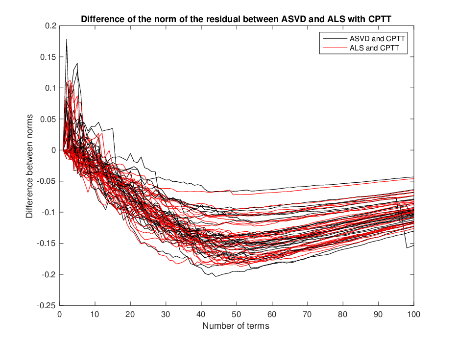


Whereas at dimension 4 (Figure 2) ALS outperforms both ASVD and CP-TT, at dimensions and (figures 3 and 4 respectively) CP-TT is featured by a better behavior. In particular, the compression rate is better on average and the decrease of the norm of the error with respect to the rank of the approximation is more regular. To better highlight this, on the right-hand side of figures 2, 3 and 4 we plot the difference of the error norms of ALS and CP-TT and ASVD and CP-TT as function of the rank of the approximation.
In the previous test a relaxed version of ALS (standard ALS with more flexibility in the scalar products in order to optimize the coefficients) was used that is observed to converge more often than the standard version of ALS. In Figure 5, the relaxed and the non relaxed version of the ALS algorithm in the 12-dimensional case are compared. Both versions were observed to yield similar compression behavior.


The results for functions, when changing the dimension, are reported in 1. In particular, we show the mean and the standard deviation of the error (on the 32 random functions) when the approximation rank is for ALS, ASVD and CP-TT. From the results, we can see that for low-order tensors (e.g. when ) ALS has better performances, whereas for higher order tensors CP-TT outperforms the other methods both in terms of mean and standard deviation (suggesting that it somehow enjoys a certain stability).
| Mean | Standard deviation | ||||||
| Dimension () | Rank () | ALS | CPTT | ASVD | ALS | CPTT | ASVD |
| 25 | 0.2942 | 0.3826 | 0.3118 | 0.0702 | 0.0850 | 0.0843 | |
| 4 | 50 | 0.1082 | 0.2433 | 0.1257 | 0.0326 | 0.0568 | 0.0664 |
| 75 | 0.0508 | 0.1681 | 0.0689 | 0.0180 | 0.0408 | 0.0666 | |
| 25 | 0.4479 | 0.3771 | 0.4806 | 0.1099 | 0.0826 | 0.1074 | |
| 6 | 50 | 0.2705 | 0.1982 | 0.2883 | 0.0752 | 0.0485 | 0.0675 |
| 75 | 0.1232 | 0.0806 | 0.1369 | 0.0325 | 0.0252 | 0.0368 | |
| 25 | 0.5341 | 0.3707 | 0.5532 | 0.1183 | 0.0592 | 0.1238 | |
| 8 | 50 | 0.3060 | 0.1909 | 0.3415 | 0.0722 | 0.0341 | 0.0932 |
| 75 | 0.1592 | 0.0682 | 0.1807 | 0.0435 | 0.0160 | 0.0625 | |
| 25 | 0.5023 | 0.3598 | 0.5451 | 0.0879 | 0.0643 | 0.1055 | |
| 10 | 50 | 0.3191 | 0.1826 | 0.3797 | 0.0643 | 0.0342 | 0.0774 |
| 75 | 0.1714 | 0.0655 | 0.2792 | 0.0453 | 0.0162 | 0.1265 | |
| 25 | 0.5170 | 0.3246 | 0.5639 | 0.1117 | 0.0576 | 0.1250 | |
| 12 | 50 | 0.3249 | 0.1623 | 0.4206 | 0.0824 | 0.0286 | 0.1579 |
| 75 | 0.1543 | 0.0579 | 0.3498 | 0.0369 | 0.0113 | 0.2057 | |
| 25 | 0.4443 | 0.2336 | 0.4783 | 0.1712 | 0.1064 | 0.1585 | |
| 14 | 50 | 0.2407 | 0.1004 | 0.3307 | 0.0937 | 0.0588 | 0.1737 |
| 75 | 0.1411 | 0.0321 | 0.2230 | 0.0541 | 0.0235 | 0.1821 | |
| 25 | 0.5529 | 0.3160 | 0.6150 | 0.1305 | 0.0818 | 0.1656 | |
| 16 | 50 | 0.3487 | 0.1448 | 0.4424 | 0.0849 | 0.0389 | 0.1942 |
| 75 | 0.1946 | 0.0616 | 0.3678 | 0.0905 | 0.0289 | 0.2354 |
4.2 Results for functions in
The method is applied to test cases in which the functions belong to , namely when the value of the parameter is chosen to be equal to . The Figures 6,7,8 are the counterpart of Figures 2,3,5 introduced and commented in the previous section.
The results obtained on functions are equivalent to the ones shown for functions, showing that the decrease in the error norm with the approximation rank is quite regular in CP-TT and behaves in a quite stable way also for higher order tensors.


The 2 collects the results for functions in .
| Mean | Standard deviation | ||||||
| Dimension () | Rank () | ALS | CPTT | ASVD | ALS | CPTT | ASVD |
| 25 | 0.1722 | 0.2261 | 0.1759 | 0.0643 | 0.2261 | 0.1759 | |
| 4 | 50 | 0.0572 | 0.1382 | 0.0590 | 0.0220 | 0.1382 | 0.0232 |
| 75 | 0.0252 | 0.0948 | 0.0262 | 0.0103 | 0.0948 | 0.0110 | |
| 25 | 0.3741 | 0.2938 | 0.4171 | 0.1158 | 0.0942 | 0.1341 | |
| 6 | 50 | 0.2037 | 0.1507 | 0.2281 | 0.0655 | 0.0523 | 0.0791 |
| 75 | 0.0851 | 0.0579 | 0.1045 | 0.0334 | 0.0233 | 0.0493 | |
| 25 | 0.3676 | 0.2560 | 0.3977 | 0.1361 | 0.0905 | 0.1517 | |
| 8 | 50 | 0.2136 | 0.1229 | 0.2413 | 0.0807 | 0.0451 | 0.1023 |
| 75 | 0.1046 | 0.0455 | 0.1145 | 0.0437 | 0.0195 | 0.0631 | |
| 25 | 0.4574 | 0.3737 | 0.4753 | 0.1235 | 0.1548 | 0.1817 | |
| 10 | 50 | 0.2613 | 0.3483 | 0.3193 | 0.0809 | 0.1825 | 0.1648 |
| 75 | 0.1168 | 0.3332 | 0.2352 | 0.0628 | 0.2034 | 0.1865 | |
| 25 | 0.4634 | 0.2505 | 0.5182 | 0.1681 | 0.0842 | 0.2116 | |
| 12 | 50 | 0.2889 | 0.1141 | 0.3922 | 0.1421 | 0.0384 | 0.2170 |
| 75 | 0.1278 | 0.0382 | 0.3144 | 0.0671 | 0.0126 | 0.2502 | |
| 25 | 0.5943 | 0.2169 | 0.4386 | 0.2043 | 0.1262 | 0.2014 | |
| 14 | 50 | 0.2841 | 0.0779 | 0.3132 | 0.1277 | 0.0686 | 0.1915 |
| 75 | 0.1422 | 0.0244 | 0.2021 | 0.0814 | 0.0227 | 0.2192 | |
| 25 | 0.4598 | 0.2460 | 0.5543 | 0.1496 | 0.0726 | 0.1603 | |
| 16 | 50 | 0.2861 | 0.1108 | 0.3936 | 0.1268 | 0.0348 | 0.2022 |
| 75 | 0.1395 | 0.0438 | 0.3181 | 0.0552 | 0.0153 | 0.2477 |
Remark:
Despite the fact that one iteration of CP-TT is in general more costly from a computational standpoint with respect to an ALS iteration, at constant target error we computational cost for CP-TT is more or less equivalent (it requires a smaller rank for higher order tensors and the ALS fix point needs more time to converge). Overall, the numerical experiments results are encouraging, showing that CP-TT is a valuable alternative for high-order tensor approximation.
5 Conclusions and perspectives
In the present work, a method has been proposed to compute, given a tensor, its CP approximation. By leveraging the properties of the TT-SVD algorithm, it is possible to compute a CP decomposition in a stable way, also in the case in which we look for a generic rank update. Albeit the fact that the iterations heavily rely on the TT-SVD algorithm, the proposed strategy does not require to fix a priori the order of the variables, but it determines it through an optimization step.
Several numerical experiments are proposed in order to assess the properties of the method and compare it with ALS and ASVD methods (which are based on similar principles). The experiments suggest that the proposed method can be a valuable tool to compute a CP decomposition in high-dimensional settings, for which the method better behaved with respect to the above mentioned alternatives. The difference in terms of sparsity between CP-TT and ALS and ASVD methods is large, and even larger for more regular functions, presenting all the CP-TT functions much similar behavior. In order to predict the results without computing them, this has to be taken into account.
The main perspectives of the present work consists in using CP-TT in the solution of multi-linear problems and to investigate how some of the defining steps of this method could be exploited in other tensor formats.
Acknowledgments
Virginie Ehrlacher acknowledges support from the ANR COMODO project (ANR-19-CE46-0002).
Damiano Lombardi acknowledges support from the ANR ADAPT project (ANR-18-CE46-0001).
This publication is part of a project that has received funding from the European Research Council (ERC) under the European Union’s Horizon 2020 Research and Innovation Programme – Grant Agreement 810367.
References
- [1] Roland Badeau and Rémy Boyer. Fast multilinear singular value decomposition for structured tensors. SIAM Journal on Matrix Analysis and Applications, 30(3):1008–1021, 2008.
- [2] Gregory Beylkin and Martin J. Mohlenkamp. Algorithms for numerical analysis in high dimensions. SIAM J. SCI. COMPUT, 26:2133–2159, 2005.
- [3] Daniele Bigoni, Allan P Engsig-Karup, and Youssef M Marzouk. Spectral tensor-train decomposition. SIAM Journal on Scientific Computing, 38(4):A2405–A2439, 2016.
- [4] A. Cichocki, N. Lee, I. Oseledets, A. Phan amd Q. Zhaonand, and D. Mandic. Tensor networks for dimensionality reduction and large-scale optimization: Part 1 low-rank tensor decompositions. Now Publishers Inc., 35, December 2016.
- [5] Andrzej Cichocki, Namgil Lee, Ivan Oseledets, Anh-Huy Phan, Qibin Zhao, and Danilo P Mandic. Tensor networks for dimensionality reduction and large-scale optimization: Part 1 low-rank tensor decompositions. Foundations and Trends® in Machine Learning, 9(4-5):249–429, 2016.
- [6] Lieven De Lathauwer, Bart De Moor, and Joos Vandewalle. A multilinear singular value decomposition. SIAM journal on Matrix Analysis and Applications, 21(4):1253–1278, 2000.
- [7] Vin de Silva and Lek-Heng Lim. Tensor rank and the ill-posedness of the best low-rank approximation problem. SIAM Journal on Matrix Analysis and Applications, 30(3):1084–1127, June 2008.
- [8] Vin De Silva and Lek-Heng Lim. Tensor rank and the ill-posedness of the best low-rank approximation problem. SIAM Journal on Matrix Analysis and Applications, 30(3):1084–1127, 2008.
- [9] I. Domanov and L. Lathauwer. On uniqueness and computation of the decomposition of a tensor into multilinear rank-(1, lr, lr) terms. SIAM J. Matrix Anal. Appl., 41:747–803, 2020.
- [10] I. Domanov and L. De Lathauwer. Canonical polyadic decomposition of third-order tensors: reduction to generalized eigenvalue decomposition. SIAM Journal on Matrix Analysis and Applications, 35(2):636–660, December 2014.
- [11] Mike Espig, Wolfgang Hackbusch, and Aram Khachatryan. On the convergence of alternating least squares optimisation in tensor format representations. arXiv preprint arXiv:1506.00062, 2015.
- [12] S. Friedland and G. Ottaviani. The number of singular vector tuples and uniqueness of best rank-one approximation of tensors. Found Comput Math, 14:1209–1242, March 2014.
- [13] Shmuel Friedland, Volker Mehrmann, Renato Pajarola, and Susanne K Suter. On best rank one approximation of tensors. Numerical Linear Algebra with Applications, 20(6):942–955, 2013.
- [14] Lars Grasedyck, Daniel Kressner, and Christine Tobler. A literature survey of low-rank tensor approximation techniques. GAMM-Mitteilungen, 36(1):53–78, 2013.
- [15] Oguz Kaya and Bora Uçar. Scalable sparse tensor decompositions in distributed memory systems. In SC’15: Proceedings of the International Conference for High Performance Computing, Networking, Storage and Analysis, pages 1–11. IEEE, 2015.
- [16] T. Kolda and B. Bader. Tensor decompositions and applications. SIAM Review, 51:455–500, 2009.
- [17] Tamara G Kolda. Tensor decomposition: A mathematical tool for data analysis. Technical report, Sandia National Lab.(SNL-CA), Livermore, CA (United States), 2018.
- [18] Tamara G Kolda and Jimeng Sun. Scalable tensor decompositions for multi-aspect data mining. In 2008 Eighth IEEE international conference on data mining, pages 363–372. IEEE, 2008.
- [19] Kirandeep Kour, Sergey Dolgov, Martin Stoll, and Peter Benner. Efficient structure-preserving support tensor train machine. arXiv preprint arXiv:2002.05079, 2020.
- [20] I. Oseledets. Tensor-train decomposition. SIAM J. Sci. Comput., 33:2295–2317, 2011.
- [21] I.V. Oseledets and E.E. Tyrtyshnikov. Breaking the curse of dimensionality, or how to use svd in many dimensions. SIAM Journal on Matrix Analysis and Applications, 31(5):1084–1127, January 2009.
- [22] Ivan V Oseledets, Maxim V Rakhuba, and André Uschmajew. Alternating least squares as moving subspace correction. SIAM Journal on Numerical Analysis, 56(6):3459–3479, 2018.
- [23] Anh-Huy Phan, Konstantin Sobolev, Konstantin Sozykin, Dmitry Ermilov, Julia Gusak, Petr Tichavsky, Valeriy Glukhov, Ivan Oseledets, and Andrzej Cichocki. Stable low-rank tensor decomposition for compression of convolutional neural network. ECCV2020, August 2020.
- [24] Anh-Huy Phan, Petr Tichavskỳ, and Andrzej Cichocki. Fast alternating ls algorithms for high order candecomp/parafac tensor factorizations. IEEE Transactions on Signal Processing, 61(19):4834–4846, 2013.
- [25] M. Rajih, P. Comon, and R. Harsman. Enhanced line search: A novel method to accelerate parafac. SIAM Journal on Matrix Analysis and Applications, 30, September 2008.
- [26] Maxim Rakhuba and Ivan Oseledets. Calculating vibrational spectra of molecules using tensor train decomposition. The Journal of Chemical Physics, 145(12):124101, 2016.
- [27] Thorsten Rohwedder and André Uschmajew. On local convergence of alternating schemes for optimization of convex problems in the tensor train format. SIAM Journal on Numerical Analysis, 51(2):1134–1162, 2013.
- [28] André Uschmajew. Local convergence of the alternating least squares algorithm for canonical tensor approximation. SIAM Journal on Matrix Analysis and Applications, 33(2):639–652, 2012.
- [29] M. Vandecappelle, N. Vervliet, and L. De Lathauwer. Nonlinear least squares updating of the canonical polyadic decomposition. In 2017 25th European Signal Processing Conference (EUSIPCO), pages 663–667, 2017.
- [30] Nico Vervliet, Otto Debals, and Lieven De Lathauwer. Exploiting efficient representations in large-scale tensor decompositions. SIAM Journal on Scientific Computing, 41(2):A789–A815, 2019.
- [31] Xiaofei Wang, Carmeliza Navasca, and Stefan Kindermann. On accelerating the regularized alternating least square algorithm for tensors. arXiv preprint arXiv:1507.04721, 2015.
- [32] Xiaokang Wang, Laurence T Yang, Yihao Wang, Xingang Liu, Qingxia Zhang, and M Jamal Deen. A distributed tensor-train decomposition method for cyber-physical-social services. ACM Transactions on Cyber-Physical Systems, 3(4):1–15, 2019.